In the previous chapter, we focused on convolutional neural networks (CNNs). We covered the building blocks of CNN architectures and how to implement deep CNNs in TensorFlow. Finally, you learned how to use CNNs for image classification. In this chapter, we will explore recurrent neural networks (RNNs) and see their application in modeling sequential data.

We will cover the following topics:

• Introducing sequential data
• RNNs for modeling sequences
• Long short-term memory (LSTM)
• Truncated backpropagation through time (TBPTT)
• Implementing a multilayer RNN for sequence modeling in TensorFlow
• Project one: RNN sentiment analysis of the IMDb movie review dataset
• Project two: RNN character-level language modeling with LSTM cells, using text data from Jules Verne's The Mysterious Island
• Using gradient clipping to avoid exploding gradients
• Introducing the Transformer model and understanding the self-attention mechanism

Introducing sequential data

Let's begin our discussion of RNNs by looking at the nature of sequential data, which is more commonly known as sequence data or sequences. We will take a look at the unique properties of sequences that make them different to other kinds of data. We will then see how we can represent sequential data and explore the various categories of models for sequential data, which are based on the input and output of a model. This will help us to explore the relationship between RNNs and sequences in this chapter.

Modeling sequential data – order matters

What makes sequences unique, compared to other types of data, is that elements in a sequence appear in a certain order and are not independent of each other. Typical machine learning algorithms for supervised learning assume that the input is independent and identically distributed (IID) data, which means that the training examples are mutually independent and have the same underlying distribution. In this regard, based on the mutual independence assumption, the order in which the training examples are given to the model is irrelevant. For example, if we have a sample consisting of n training examples, , the order in which we use the data for training our machine learning algorithm does not matter. An example of this scenario would be the Iris dataset that we previously worked with. In the Iris dataset, each flower has been measured independently, and the measurements of one flower do not influence the measurements of another flower.

However, this assumption is not valid when we deal with sequences—by definition, order matters. Predicting the market value of a particular stock would be an example of this scenario. For instance, assume we have a sample of n training examples, where each training example represents the market value of a certain stock on a particular day. If our task is to predict the stock market value for the next three days, it would make sense to consider the previous stock prices in a date-sorted order to derive trends rather than utilize these training examples in a randomized order.

Representing sequences

We've established that order among data points is important in sequential data, so we next need to find a way to leverage this ordering information in a machine learning model. Throughout this chapter, we will represent sequences as . The superscript indices indicate the order of the instances, and the length of the sequence is T. For a sensible example of sequences, consider time-series data, where each example point, , belongs to a particular time, t. The following figure shows an example of time-series data where both the input features (x's) and the target labels (y's) naturally follow the order according to their time axis; therefore, both the x's and y's are sequences:

As we have already mentioned, the standard neural network (NN) models that we have covered so far, such as multilayer perceptron (MLP) and CNNs for image data, assume that the training examples are independent of each other and thus do not incorporate ordering information. We can say that such models do not have a memory of previously seen training examples. For instance, the samples are passed through the feedforward and backpropagation steps, and the weights are updated independently of the order in which the training examples are processed.

RNNs, by contrast, are designed for modeling sequences and are capable of remembering past information and processing new events accordingly, which is a clear advantage when working with sequence data.

The different categories of sequence modeling

Sequence modeling has many fascinating applications, such as language translation (for example, translating text from English to German), image captioning, and text generation. However, in order to choose an appropriate architecture and approach, we have to understand and be able to distinguish between these different sequence modeling tasks. The following figure, based on the explanations in the excellent article The Unreasonable Effectiveness of Recurrent Neural Networks, by Andrej Karpathy (http://karpathy.github.io/2015/05/21/rnn-effectiveness/), summarizes the most common sequence modeling tasks, which depend on the relationship categories of input and output data:

Let's discuss the different relationship categories between input and output data, which were depicted in the previous figure, in more detail. If neither the input nor output data represents sequences, then we are dealing with standard data, and we could simply use a multilayer perceptron (or another classification model previously covered in this book) to model such data. However, if either the input or output is a sequence, the modeling task likely falls into one of these categories:

• Many-to-one: The input data is a sequence, but the output is a fixed-size vector or scalar, not a sequence. For example, in sentiment analysis, the input is text-based (for example, a movie review) and the output is a class label (for example, a label denoting whether a reviewer liked the movie).
• One-to-many: The input data is in standard format and not a sequence, but the output is a sequence. An example of this category is image captioning—the input is an image and the output is an English phrase summarizing the content of that image.
• Many-to-many: Both the input and output arrays are sequences. This category can be further divided based on whether the input and output are synchronized. An example of a synchronized many-to-many modeling task is video classification, where each frame in a video is labeled. An example of a delayed many-to-many modeling task would be translating one language into another. For instance, an entire English sentence must be read and processed by a machine before its translation into German is produced.

Now, after summarizing the three broad categories of sequence modeling, we can move forward to discussing the structure of an RNN.

RNNs for modeling sequences

In this section, before we start implementing RNNs in TensorFlow, we will discuss the main concepts of RNNs. We will begin by looking at the typical structure of an RNN, which includes a recursive component to model sequence data. Then, we will examine how the neuron activations are computed in a typical RNN. This will create a context for us to discuss the common challenges in training RNNs, and we will then discuss solutions to these challenges, such as LSTM and gated recurrent units (GRUs).

Understanding the RNN looping mechanism

Let's start with the architecture of an RNN. The following figure shows a standard feedforward NN and an RNN side by side for comparison:

Both of these networks have only one hidden layer. In this representation, the units are not displayed, but we assume that the input layer (x), hidden layer (h), and output layer (o) are vectors that contain many units.

In a standard feedforward network, information flows from the input to the hidden layer, and then from the hidden layer to the output layer. On the other hand, in an RNN, the hidden layer receives its input from both the input layer of the current time step and the hidden layer from the previous time step.

The flow of information in adjacent time steps in the hidden layer allows the network to have a memory of past events. This flow of information is usually displayed as a loop, also known as a recurrent edge in graph notation, which is how this general RNN architecture got its name.

Similar to multilayer perceptrons, RNNs can consist of multiple hidden layers. Note that it's a common convention to refer to RNNs with one hidden layer as a single-layer RNN, which is not to be confused with single-layer NNs without a hidden layer, such as Adaline or logistic regression. The following figure illustrates an RNN with one hidden layer (top) and an RNN with two hidden layers (bottom):

In order to examine the architecture of RNNs and the flow of information, a compact representation with a recurrent edge can be unfolded, which you can see in the preceding figure.

As we know, each hidden unit in a standard NN receives only one input—the net preactivation associated with the input layer. In contrast, each hidden unit in an RNN receives two distinct sets of input—the preactivation from the input layer and the activation of the same hidden layer from the previous time step, t – 1.

At the first time step, t = 0, the hidden units are initialized to zeros or small random values. Then, at a time step where t > 0, the hidden units receive their input from the data point at the current time, , and the previous values of hidden units at t – 1, indicated as .

Similarly, in the case of a multilayer RNN, we can summarize the information flow as follows:

• layer = 1: Here, the hidden layer is represented as and it receives its input from the data point, , and the hidden values in the same layer, but at the previous time step, .
• layer = 2: The second hidden layer, , receives its inputs from the outputs of the layer below at the current time step () and its own hidden values from the previous time step, .

Since, in this case, each recurrent layer must receive a sequence as input, all the recurrent layers except the last one must return a sequence as output (that is, return_sequences=True). The behavior of the last recurrent layer depends on the type of problem.

Computing activations in an RNN

Now that you understand the structure and general flow of information in an RNN, let's get more specific and compute the actual activations of the hidden layers, as well as the output layer. For simplicity, we will consider just a single hidden layer; however, the same concept applies to multilayer RNNs.

Each directed edge (the connections between boxes) in the representation of an RNN that we just looked at is associated with a weight matrix. Those weights do not depend on time, t; therefore, they are shared across the time axis. The different weight matrices in a single-layer RNN are as follows:

• : The weight matrix between the input, , and the hidden layer, h
• : The weight matrix associated with the recurrent edge
• : The weight matrix between the hidden layer and output layer

These weight matrices are depicted in the following figure:

In certain implementations, you may observe that the weight matrices, and , are concatenated to a combined matrix, . Later in this section, we will make use of this notation as well.

Computing the activations is very similar to standard multilayer perceptrons and other types of feedforward NNs. For the hidden layer, the net input, (preactivation), is computed through a linear combination, that is, we compute the sum of the multiplications of the weight matrices with the corresponding vectors and add the bias unit:

Then, the activations of the hidden units at the time step, t, are calculated as follows:

Here, is the bias vector for the hidden units and is the activation function of the hidden layer.

In case you want to use the concatenated weight matrix, , the formula for computing hidden units will change, as follows:

Once the activations of the hidden units at the current time step are computed, then the activations of the output units will be computed, as follows:

To help clarify this further, the following figure shows the process of computing these activations with both formulations:

Hidden-recurrence versus output-recurrence

So far, you have seen recurrent networks in which the hidden layer has the recurrent property. However, note that there is an alternative model in which the recurrent connection comes from the output layer. In this case, the net activations from the output layer at the previous time step, , can be added in one of two ways:

• To the hidden layer at the current time step, (shown in the following figure as output-to-hidden recurrence)
• To the output layer at the current time step, (shown in the following figure as output-to-output recurrence)

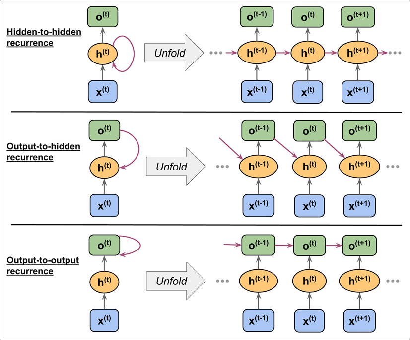
As shown in the previous figure, the differences between these architectures can be clearly seen in the recurring connections. Following our notation, the weights associated with the recurrent connection will be denoted for the hidden-to-hidden recurrence by , for the output-to-hidden recurrence by , and for the output-to-output recurrence by . In some articles in literature, the weights associated with the recurrent connections are also denoted by .

To see how this works in practice, let's manually compute the forward pass for one of these recurrent types. Using the TensorFlow Keras API, a recurrent layer can be defined via SimpleRNN, which is similar to the output-to-output recurrence. In the following code, we will create a recurrent layer from SimpleRNN and perform a forward pass on an input sequence of length 3 to compute the output. We will also manually compute the forward pass and compare the results with those of SimpleRNN. First, let's create the layer and assign the weights for our manual computations:

>>> import tensorflow as tf
>>> tf.random.set_seed(1)
>>> rnn_layer = tf.keras.layers.SimpleRNN(
...     units=2, use_bias=True,
...     return_sequences=True)
>>> rnn_layer.build(input_shape=(None, None, 5))
>>> w_xh, w_oo, b_h = rnn_layer.weights
>>> print('W_xh shape:', w_xh.shape)
>>> print('W_oo shape:', w_oo.shape)
>>> print('b_h  shape:', b_h.shape)
W_xh shape: (5, 2)
W_oo shape: (2, 2)
b_h  shape: (2,)

The input shape for this layer is (None, None, 5), where the first dimension is the batch dimension (using None for variable batch size), the second dimension corresponds to the sequence (using None for the variable sequence length), and the last dimension corresponds to the features. Notice that we set return_sequences=True, which, for an input sequence of length 3, will result in the output sequence . Otherwise, it would only return the final output, .

Now, we will call the forward pass on the rnn_layer and manually compute the outputs at each time step and compare them:

>>> x_seq = tf.convert_to_tensor(
...     [[1.0]*5, [2.0]*5, [3.0]*5],
...     dtype=tf.float32)
>>> ## output of SimepleRNN:
>>> output = rnn_layer(tf.reshape(x_seq, shape=(1, 3, 5)))
>>> ## manually computing the output:
>>> out_man = []
>>> for t in range(len(x_seq)):
...     xt = tf.reshape(x_seq[t], (1, 5))
...     print('Time step {} =>'.format(t))
...     print('   Input           :', xt.numpy())
...     
...     ht = tf.matmul(xt, w_xh) + b_h
...     print('   Hidden          :', ht.numpy())
...     
...     if t>0:
...         prev_o = out_man[t-1]
...     else:
...         prev_o = tf.zeros(shape=(ht.shape))
...     ot = ht + tf.matmul(prev_o, w_oo)
...     ot = tf.math.tanh(ot)
...     out_man.append(ot)
...     print('   Output (manual) :', ot.numpy())
...     print('   SimpleRNN output:'.format(t),
...           output[0][t].numpy())
...     print()
Time step 0 =>
   Input           : [[1. 1. 1. 1. 1.]]
   Hidden          : [[0.41464037 0.96012145]]
   Output (manual) : [[0.39240566 0.74433106]]
   SimpleRNN output: [0.39240566 0.74433106]
Time step 1 =>
   Input           : [[2. 2. 2. 2. 2.]]
   Hidden          : [[0.82928073 1.9202429 ]]
   Output (manual) : [[0.80116504 0.9912947 ]]
   SimpleRNN output: [0.80116504 0.9912947 ]
Time step 2 =>
   Input           : [[3. 3. 3. 3. 3.]]
   Hidden          : [[1.243921  2.8803642]]
   Output (manual) : [[0.95468265 0.9993069 ]]
   SimpleRNN output: [0.95468265 0.9993069 ]

In our manual forward computation, we used the hyperbolic tangent (tanh) activation function, since it is also used in SimpleRNN (the default activation). As you can see from the printed results, the outputs from the manual forward computations exactly match the output of the SimpleRNN layer at each time step. Hopefully, this hands-on task has enlightened you on the mysteries of recurrent networks.

The challenges of learning long-range interactions

BPTT, which was briefly mentioned earlier, introduces some new challenges. Because of the multiplicative factor, , in computing the gradients of a loss function, the so-called vanishing and exploding gradient problems arise. These problems are explained by the examples in the following figure, which shows an RNN with only one hidden unit for simplicity:

Basically, has t – k multiplications; therefore, multiplying the weight, w, by itself t – k times results in a factor, . As a result, if , this factor becomes very small when t – k is large. On the other hand, if the weight of the recurrent edge is , then becomes very large when t – k is large. Note that large t – k refers to long-range dependencies. We can see that a naive solution to avoid vanishing or exploding gradients can be reached by ensuring . If you are interested and would like to investigate this in more detail, read On the difficulty of training recurrent neural networks, by R. Pascanu, T. Mikolov, and Y. Bengio, 2012 (https://arxiv.org/pdf/1211.5063.pdf).

In practice, there are at least three solutions to this problem:

• Gradient clipping
• TBPTT
• LSTM

Using gradient clipping, we specify a cut-off or threshold value for the gradients, and we assign this cut-off value to gradient values that exceed this value. In contrast, TBPTT simply limits the number of time steps that the signal can backpropagate after each forward pass. For example, even if the sequence has 100 elements or steps, we may only backpropagate the most recent 20 time steps.

While both gradient clipping and TBPTT can solve the exploding gradient problem, the truncation limits the number of steps that the gradient can effectively flow back and properly update the weights. On the other hand, LSTM, designed in 1997 by Sepp Hochreiter and Jürgen Schmidhuber, has been more successful in vanishing and exploding gradient problems while modeling long-range dependencies through the use of memory cells. Let's discuss LSTM in more detail.

Long short-term memory cells

As stated previously, LSTMs were first introduced to overcome the vanishing gradient problem (Long Short-Term Memory, S. Hochreiter and J. Schmidhuber, Neural Computation, 9(8): 1735-1780, 1997). The building block of an LSTM is a memory cell, which essentially represents or replaces the hidden layer of standard RNNs.

In each memory cell, there is a recurrent edge that has the desirable weight, w = 1, as we discussed, to overcome the vanishing and exploding gradient problems. The values associated with this recurrent edge are collectively called the cell state. The unfolded structure of a modern LSTM cell is shown in the following figure:

Notice that the cell state from the previous time step, , is modified to get the cell state at the current time step, , without being multiplied directly with any weight factor. The flow of information in this memory cell is controlled by several computation units (often called gates) that will be described here. In the previous figure, refers to the element-wise product (element-wise multiplication) and means element-wise summation (element-wise addition). Furthermore, refers to the input data at time t, and indicates the hidden units at time t – 1. Four boxes are indicated with an activation function, either the sigmoid function () or tanh, and a set of weights; these boxes apply a linear combination by performing matrix-vector multiplications on their inputs (which are and ). These units of computation with sigmoid activation functions, whose output units are passed through , are called gates.

In an LSTM cell, there are three different types of gates, which are known as the forget gate, the input gate, and the output gate:

• The forget gate ( ) allows the memory cell to reset the cell state without growing indefinitely. In fact, the forget gate decides which information is allowed to go through and which information to suppress. Now, is computed as follows:

  

  Note that the forget gate was not part of the original LSTM cell; it was added a few years later to improve the original model (Learning to Forget: Continual Prediction with LSTM, F. Gers, J. Schmidhuber, and F. Cummins, Neural Computation 12, 2451-2471, 2000).

• The input gate () and candidate value () are responsible for updating the cell state. They are computed as follows:

  

  

  The cell state at time t is computed as follows:

  

• The output gate () decides how to update the values of hidden units:

  

  Given this, the hidden units at the current time step are computed as follows:

  

The structure of an LSTM cell and its underlying computations might seem very complex and hard to implement. However, the good news is that TensorFlow has already implemented everything in optimized wrapper functions, which allows us to define our LSTM cells easily and efficiently. We will apply RNNs and LSTMs to real-world datasets later in this chapter.

Implementing RNNs for sequence modeling in TensorFlow

Now that we have covered the underlying theory behind RNNs, we are ready to move on to the more practical portion of this chapter: implementing RNNs in TensorFlow. During the rest of this chapter, we will apply RNNs to two common problem tasks:

1. Sentiment analysis
2. Language modeling

These two projects, which we will walk through together in the following pages, are both fascinating but also quite involved. Thus, instead of providing the code all at once, we will break the implementation up into several steps and discuss the code in detail. If you like to have a big picture overview and want to see all the code at once before diving into the discussion, take a look at the code implementation first, which you can view at https://github.com/rasbt/python-machine-learning-book-3rd-edition/tree/master/ch16.

Project one – predicting the sentiment of IMDb movie reviews

You may recall from Chapter 8, Applying Machine Learning to Sentiment Analysis, that sentiment analysis is concerned with analyzing the expressed opinion of a sentence or a text document. In this section and the following subsections, we will implement a multilayer RNN for sentiment analysis using a many-to-one architecture.

In the next section, we will implement a many-to-many RNN for an application of language modeling. While the chosen examples are purposefully simple to introduce the main concepts of RNNs, language modeling has a wide range of interesting applications, such as building chatbots—giving computers the ability to directly talk and interact with humans.

Preparing the movie review data

In the preprocessing steps in Chapter 8, we created a clean dataset named movie_data.csv, which we will use again now. First, we will import the necessary modules and read the data into a pandas DataFrame, as follows:

>>> import tensorflow as tf
>>> import tensorflow_datasets as tfds
>>> import numpy as np
>>> import pandas as pd
>>> df = pd.read_csv('movie_data.csv', encoding='utf-8')

Remember that this data frame, df, consists of two columns, namely 'review' and 'sentiment', where 'review' contains the text of movie reviews (the input features), and 'sentiment' represents the target label we want to predict (0 refers to negative sentiment and 1 refers to positive sentiment). The text component of these movie reviews is sequences of words, and the RNN model classifies each sequence as a positive (1) or negative (0) review.

However, before we can feed the data into an RNN model, we need to apply several preprocessing steps:

1. Create a TensorFlow dataset object and split it into separate training, testing, and validation partitions.
2. Identify the unique words in the training dataset.
3. Map each unique word to a unique integer and encode the review text into encoded integers (an index of each unique word).
4. Divide the dataset into mini-batches as input to the model.

Let's proceed with the first step: creating a TensorFlow dataset from this data frame:

>>> ## Step 1: create a dataset
>>> target = df.pop('sentiment')
>>> ds_raw = tf.data.Dataset.from_tensor_slices(
...     (df.values, target.values))
>>> ## inspection:
>>> for ex in ds_raw.take(3):
...     tf.print(ex[0].numpy()[0][ :50], ex[1])
b'In 1974, the teenager Martha Moxley (Maggie Grace)' 1
b'OK... so... I really like Kris Kristofferson and h' 0
b'***SPOILER*** Do not read this, if you think about' 0

Now, we can split it into training, testing, and validation datasets. The entire dataset contains 50,000 examples. We will keep the first 25,000 examples for evaluation (hold-out testing dataset), and then 20,000 examples will be used for training and 5,000 for validation. The code is as follows:

>>> tf.random.set_seed(1)
>>> ds_raw = ds_raw.shuffle(
...     50000, reshuffle_each_iteration=False)
>>> ds_raw_test = ds_raw.take(25000)
>>> ds_raw_train_valid = ds_raw.skip(25000)
>>> ds_raw_train = ds_raw_train_valid.take(20000)
>>> ds_raw_valid = ds_raw_train_valid.skip(20000)

To prepare the data for input to a NN, we need to encode it into numeric values, as was mentioned in steps 2 and 3. To do this, we will first find the unique words (tokens) in the training dataset. While finding unique tokens is a process for which we can use Python datasets, it can be more efficient to use the Counter class from the collections package, which is part of Python's standard library.

In the following code, we will instantiate a new Counter object (token_counts) that will collect the unique word frequencies. Note that in this particular application (and in contrast to the bag-of-words model), we are only interested in the set of unique words and won't require the word counts, which are created as a side product. To split the text into words (or tokens), the tensorflow_datasets package provides a Tokenizer class.

The code for collecting unique tokens is as follows:

>>> ## Step 2: find unique tokens (words)
>>> from collections import Counter
>>> tokenizer = tfds.features.text.Tokenizer()
>>> token_counts = Counter()
>>> for example in ds_raw_train:
...     tokens = tokenizer.tokenize(example[0].numpy()[0])
...     token_counts.update(tokens)
>>> print('Vocab-size:', len(token_counts))
Vocab-size: 87007

If you want to learn more about Counter, refer to its documentation at https://docs.python.org/3/library/collections.html#collections.Counter.

Next, we are going to map each unique word to a unique integer. This can be done manually using a Python dictionary, where the keys are the unique tokens (words) and the value associated with each key is a unique integer. However, the tensorflow_datasets package already provides a class, TokenTextEncoder, which we can use to create such a mapping and encode the entire dataset. First, we will create an encoder object from the TokenTextEncoder class by passing the unique tokens (token_counts contains the tokens and their counts, although here, their counts are not needed, so they will be ignored). Calling the encoder.encode() method will then convert its input text into a list of integer values:

>>> ## Step 3: encoding unique tokens to integers
>>> encoder = tfds.features.text.TokenTextEncoder(token_counts)
>>> example_str = 'This is an example!'
>>> print(encoder.encode(example_str))
[232, 9, 270, 1123]

Note that there might be some tokens in the validation or testing data that are not present in the training data and are thus not included in the mapping. If we have q tokens (that is the size of token_counts passed to the TokenTextEncoder, which in this case is 87,007), then all tokens that haven't been seen before, and are thus not included in token_counts, will be assigned the integer q + 1 (which will be 87,008 in our case). In other words, the index q + 1 is reserved for unknown words. Another reserved value is the integer 0, which serves as a placeholder for adjusting the sequence length. Later, when we are building an RNN model in TensorFlow, we will consider these two placeholders, 0 and q + 1, in more detail.

We can use the map() method of the dataset objects to transform each text in the dataset accordingly, just like we would apply any other transformation to a dataset. However, there is a small problem: here, the text data is enclosed in tensor objects, which we can access by calling the numpy() method on a tensor in the eager execution mode. But during transformations by the map() method, the eager execution will be disabled. To solve this problem, we can define two functions. The first function will treat the input tensors as if the eager execution mode is enabled:

>>> ## Step 3-A: define the function for transformation
>>> def encode(text_tensor, label):
...     text = text_tensor.numpy()[0]
...     encoded_text = encoder.encode(text)
...     return encoded_text, label

In the second function, we will wrap the first function using tf.py_function to convert it into a TensorFlow operator, which can then be used via its map() method. This process of encoding text into a list of integers can be carried out using the following code:

>>> ## Step 3-B: wrap the encode function to a TF Op.
>>> def encode_map_fn(text, label):
...     return tf.py_function(encode, inp=[text, label],
...                           Tout=(tf.int64, tf.int64))
>>> ds_train = ds_raw_train.map(encode_map_fn)
>>> ds_valid = ds_raw_valid.map(encode_map_fn)
>>> ds_test = ds_raw_test.map(encode_map_fn)
>>> # look at the shape of some examples:
>>> tf.random.set_seed(1)
>>> for example in ds_train.shuffle(1000).take(5):
...     print('Sequence length:', example[0].shape)
Sequence length: (24,)
Sequence length: (179,)
Sequence length: (262,)
Sequence length: (535,)
Sequence length: (130,)

So far, we've converted sequences of words into sequences of integers. However, there is one issue that we still need to resolve—the sequences currently have different lengths (as shown in the result of executing the previous code for five randomly chosen examples). Although, in general, RNNs can handle sequences with different lengths, we still need to make sure that all the sequences in a mini-batch have the same length to store them efficiently in a tensor.

To divide a dataset that has elements with different shapes into mini-batches, TensorFlow provides a different method, padded_batch() (instead of batch()), which will automatically pad the consecutive elements that are to be combined into a batch with placeholder values (0s) so that all sequences within a batch will have the same shape. To illustrate this with a practical example, let's take a small subset of size 8 from the training dataset, ds_train, and apply the padded_batch() method to this subset with batch_size=4. We will also print the sizes of the individual elements before combining these into mini-batches, as well as the dimensions of the resulting mini-batches:

>>> ## Take a small subset
>>> ds_subset = ds_train.take(8)
>>> for example in ds_subset:
...     print('Individual size:', example[0].shape)
Individual size: (119,)
Individual size: (688,)
Individual size: (308,)
Individual size: (204,)
Individual size: (326,)
Individual size: (240,)
Individual size: (127,)
Individual size: (453,)
>>> ## Dividing the dataset into batches
>>> ds_batched = ds_subset.padded_batch(
...              4, padded_shapes=([-1], []))
>>> for batch in ds_batched:
...     print('Batch dimension:', batch[0].shape)
Batch dimension: (4, 688)
Batch dimension: (4, 453)

As you can observe from the printed tensor shapes, the number of columns (that is, .shape[1]) in the first batch is 688, which resulted from combining the first four examples into a single batch and using the maximum size of these examples. That means that the other three examples in this batch are padded as much as necessary to match this size. Similarly, the second batch keeps the maximum size of its individual four examples, which is 453, and pads the other examples so that their length is smaller than the maximum length.

Let's divide all three datasets into mini-batches with a batch size of 32:

>>> train_data = ds_train.padded_batch(
...     32, padded_shapes=([-1],[]))
>>> valid_data = ds_valid.padded_batch(
...     32, padded_shapes=([-1],[]))
>>> test_data = ds_test.padded_batch(
...     32, padded_shapes=([-1],[]))

Now, the data is in a suitable format for an RNN model, which we are going to implement in the following subsections. In the next subsection, however, we will first discuss feature embedding, which is an optional but highly recommended preprocessing step that is used for reducing the dimensionality of the word vectors.

Embedding layers for sentence encoding

During the data preparation in the previous step, we generated sequences of the same length. The elements of these sequences were integer numbers that corresponded to the indices of unique words. These word indices can be converted into input features in several different ways. One naive way is to apply one-hot encoding to convert the indices into vectors of zeros and ones. Then, each word will be mapped to a vector whose size is the number of unique words in the entire dataset. Given that the number of unique words (the size of the vocabulary) can be in the order of , which will also be the number of our input features, a model trained on such features may suffer from the curse of dimensionality. Furthermore, these features are very sparse, since all are zero except one.

A more elegant approach is to map each word to a vector of a fixed size with real-valued elements (not necessarily integers). In contrast to the one-hot encoded vectors, we can use finite-sized vectors to represent an infinite number of real numbers. (In theory, we can extract infinite real numbers from a given interval, for example [–1, 1].)

This is the idea behind embedding, which is a feature-learning technique that we can utilize here to automatically learn the salient features to represent the words in our dataset. Given the number of unique words, , we can select the size of the embedding vectors (a.k.a., embedding dimension) to be much smaller than the number of unique words () to represent the entire vocabulary as input features.

The advantages of embedding over one-hot encoding are as follows:

• A reduction in the dimensionality of the feature space to decrease the effect of the curse of dimensionality
• The extraction of salient features since the embedding layer in an NN can be optimized (or learned)

The following schematic representation shows how embedding works by mapping token indices to a trainable embedding matrix:

Given a set of tokens of size n + 2 (n is the size of the token set, plus index 0 is reserved for the padding placeholder, and n + 1 is for the words not present in the token set), an embedding matrix of size will be created where each row of this matrix represents numeric features associated with a token. Therefore, when an integer index, i, is given as input to the embedding, it will look up the corresponding row of the matrix at index i and return the numeric features. The embedding matrix serves as the input layer to our NN models. In practice, creating an embedding layer can simply be done using tf.keras.layers.Embedding. Let's see an example where we will create a model and add an embedding layer, as follows:

>>> from tensorflow.keras.layers import Embedding
>>> model = tf.keras.Sequential()
>>> model.add(Embedding(input_dim=100,
...                     output_dim=6,
...                     input_length=20,
...                     name='embed-layer'))
>>> model.summary()
Model: "sequential"
_________________________________________________________________
Layer (type)                 Output Shape              Param #   
=================================================================
embed-layer (Embedding)      (None, 20, 6)             600      
=================================================================
Total params: 6,00
Trainable params: 6,00
Non-trainable params: 0
_________________________________________________________________

The input to this model (embedding layer) must have rank 2 with dimensionality , where is the length of sequences (here, set to 20 via the input_length argument). For example, an input sequence in the mini-batch could be , where each element of this sequence is the index of the unique words. The output will have dimensionality , where is the size of the embedding features (here, set to 6 via output_dim). The other argument provided to the embedding layer, input_dim, corresponds to the unique integer values that the model will receive as input (for instance, n + 2, set here to 100). Therefore, the embedding matrix in this case has the size .

Building an RNN model

Now we're ready to build an RNN model. Using the Keras Sequential class, we can combine the embedding layer, the recurrent layers of the RNN, and the fully connected non-recurrent layers. For the recurrent layers, we can use any of the following implementations:

• SimpleRNN: a regular RNN layer, that is, a fully connected recurrent layer
• LSTM: a long short-term memory RNN, which is useful for capturing the long-term dependencies
• GRU: a recurrent layer with a gated recurrent unit, as proposed in Learning Phrase Representations Using RNN Encoder–Decoder for Statistical Machine Translation (https://arxiv.org/abs/1406.1078v3), as an alternative to LSTMs

To see how a multilayer RNN model can be built using one of these recurrent layers, in the following example, we will create an RNN model, starting with an embedding layer with input_dim=1000 and output_dim=32. Then, two recurrent layers of type SimpleRNN will be added. Finally, we will add a non-recurrent fully connected layer as the output layer, which will return a single output value as the prediction:

>>> from tensorflow.keras import Sequential
>>> from tensorflow.keras.layers import Embedding
>>> from tensorflow.keras.layers import SimpleRNN
>>> from tensorflow.keras.layers import Dense
>>> model = Sequential()
>>> model.add(Embedding(input_dim=1000, output_dim=32))
>>> model.add(SimpleRNN(32, return_sequences=True))
>>> model.add(SimpleRNN(32))
>>> model.add(Dense(1))
>>> model.summary()
Model: "sequential"
_________________________________________________________________
Layer (type)                 Output Shape              Param #   
=================================================================
embedding (Embedding)        (None, None, 32)          32000     
_________________________________________________________________
simple_rnn (SimpleRNN)       (None, None, 32)          2080      
_________________________________________________________________
simple_rnn_1 (SimpleRNN)     (None, 32)                2080      
_________________________________________________________________
dense (Dense)                (None, 1)                 33        
=================================================================
Total params: 36,193
Trainable params: 36,193
Non-trainable params: 0
_________________________________________________________________

As you can see, building an RNN model using these recurrent layers is pretty straightforward. In the next subsection, we will go back to our sentiment analysis task and build an RNN model to solve that.

Building an RNN model for the sentiment analysis task

Since we have very long sequences, we are going to use an LSTM layer to account for long-term effects. In addition, we will put the LSTM layer inside a Bidirectional wrapper, which will make the recurrent layers pass through the input sequences from both directions, start to end, as well as the reverse direction:

>>> embedding_dim = 20
>>> vocab_size = len(token_counts) + 2
>>> tf.random.set_seed(1)
>>> ## build the model
>>> bi_lstm_model = tf.keras.Sequential([
...     tf.keras.layers.Embedding(
...         input_dim=vocab_size,
...         output_dim=embedding_dim,
...         name='embed-layer'),
...     
...     tf.keras.layers.Bidirectional(
...         tf.keras.layers.LSTM(64, name='lstm-layer'),
...         name='bidir-lstm'),
...
...     tf.keras.layers.Dense(64, activation='relu'),
...     
...     tf.keras.layers.Dense(1, activation='sigmoid')
>>> ])
>>> bi_lstm_model.summary()
>>> ## compile and train:
>>> bi_lstm_model.compile(
...     optimizer=tf.keras.optimizers.Adam(1e-3),
...     loss=tf.keras.losses.BinaryCrossentropy(from_logits=False),
...     metrics=['accuracy'])
>>> history = bi_lstm_model.fit(
...     train_data,
...     validation_data=valid_data,
...     epochs=10)
>>> ## evaluate on the test data
>>> test_results = bi_lstm_model.evaluate(test_data)
>>> print('Test Acc.: {:.2f}%'.format(test_results[1]*100))
Epoch 1/10
625/625 [==============================] - 96s 154ms/step - loss: 0.4410 - accuracy: 0.7782 - val_loss: 0.0000e+00 - val_accuracy: 0.0000e+00
Epoch 2/10
625/625 [==============================] - 95s 152ms/step - loss: 0.1799 - accuracy: 0.9326 - val_loss: 0.4833 - val_accuracy: 0.8414
. . .
Test Acc.: 85.15%

After training this model for 10 epochs, evaluation on the test data shows 85 percent accuracy. (Note that this result is not the best when compared to the state-of-the-art methods used on the IMDb dataset. The goal was simply to show how RNN works.)

We can also try other types of recurrent layers, such as SimpleRNN. However, as it turns out, a model built with regular recurrent layers won't be able to reach a good predictive performance (even on the training data). For example, if you try replacing the bidirectional LSTM layer in the previous code with a unidirectional SimpleRNN layer and train the model on full-length sequences, you may observe that the loss will not even decrease during training. The reason is that the sequences in this dataset are too long, so a model with a SimpleRNN layer cannot learn the long-term dependencies and may suffer from vanishing or exploding gradient problems.

In order to obtain reasonable predictive performance on this dataset using a SimpleRNN, we can truncate the sequences. Also, utilizing our "domain knowledge," we may hypothesize that the last paragraphs of a movie review may contain most of the information about its sentiment. Hence, we can focus only on the last portion of each review. To do this, we will define a helper function, preprocess_datasets(), to combine the preprocessing steps 2-4. An optional argument to this function is max_seq_length, which determines how many tokens from each review should be used. For example, if we set max_seq_length=100 and a review has more than 100 tokens, only the last 100 tokens will be used. If max_seq_length is set to None, then full-length sequences will be used as before. Trying different values for max_seq_length will give us more insights on the capability of different RNN models to handle long sequences.

The code for the preprocess_datasets() function is as follows:

>>> from collections import Counter
>>> def preprocess_datasets(
...     ds_raw_train,
...     ds_raw_valid,
...     ds_raw_test,
...     max_seq_length=None,
...     batch_size=32):
...     
...     ## (step 1 is already done)
...     ## Step 2: find unique tokens
...     tokenizer = tfds.features.text.Tokenizer()
...     token_counts = Counter()
...
...     for example in ds_raw_train:
...         tokens = tokenizer.tokenize(example[0].numpy()[0])
...         if max_seq_length is not None:
...             tokens = tokens[-max_seq_length:]
...         token_counts.update(tokens)
...
...     print('Vocab-size:', len(token_counts))
...
...     ## Step 3: encoding the texts
...     encoder = tfds.features.text.TokenTextEncoder(
...                   token_counts)
...     def encode(text_tensor, label):
...         text = text_tensor.numpy()[0]
...         encoded_text = encoder.encode(text)
...         if max_seq_length is not None:
...             encoded_text = encoded_text[-max_seq_length:]
...         return encoded_text, label
...
...     def encode_map_fn(text, label):
...         return tf.py_function(encode, inp=[text, label],
...                               Tout=(tf.int64, tf.int64))
...
...     ds_train = ds_raw_train.map(encode_map_fn)
...     ds_valid = ds_raw_valid.map(encode_map_fn)
...     ds_test = ds_raw_test.map(encode_map_fn)
...
...     ## Step 4: batching the datasets
...     train_data = ds_train.padded_batch(
...         batch_size, padded_shapes=([-1],[]))
...
...     valid_data = ds_valid.padded_batch(
...         batch_size, padded_shapes=([-1],[]))
...
...     test_data = ds_test.padded_batch(
...         batch_size, padded_shapes=([-1],[]))
...
...     return (train_data, valid_data,
...             test_data, len(token_counts))

Next, we will define another helper function, build_rnn_model(), for building models with different architectures more conveniently:

>>> from tensorflow.keras.layers import Embedding
>>> from tensorflow.keras.layers import Bidirectional
>>> from tensorflow.keras.layers import SimpleRNN
>>> from tensorflow.keras.layers import LSTM
>>> from tensorflow.keras.layers import GRU
>>> def build_rnn_model(embedding_dim, vocab_size,
...                     recurrent_type='SimpleRNN',
...                     n_recurrent_units=64,
...                     n_recurrent_layers=1,
...                     bidirectional=True):
...
...     tf.random.set_seed(1)
...
...     # build the model
...     model = tf.keras.Sequential()
...     
...     model.add(
...         Embedding(
...             input_dim=vocab_size,
...             output_dim=embedding_dim,
...             name='embed-layer')
...     )
...     
...     for i in range(n_recurrent_layers):
...         return_sequences = (i < n_recurrent_layers-1)
...             
...         if recurrent_type == 'SimpleRNN':
...             recurrent_layer = SimpleRNN(
...                 units=n_recurrent_units,
...                 return_sequences=return_sequences,
...                 name='simprnn-layer-{}'.format(i))
...         elif recurrent_type == 'LSTM':
...             recurrent_layer = LSTM(
...                 units=n_recurrent_units,
...                 return_sequences=return_sequences,
...                 name='lstm-layer-{}'.format(i))
...         elif recurrent_type == 'GRU':
...             recurrent_layer = GRU(
...                 units=n_recurrent_units,
...                 return_sequences=return_sequences,
...                 name='gru-layer-{}'.format(i))
...         
...         if bidirectional:
...             recurrent_layer = Bidirectional(
...                 recurrent_layer, name='bidir-' +
...                 recurrent_layer.name)
...             
...         model.add(recurrent_layer)
...
...     model.add(tf.keras.layers.Dense(64, activation='relu'))
...     model.add(tf.keras.layers.Dense(1, activation='sigmoid'))
...     
...     return model

Now, using these two fairly general, but convenient, helper functions, we can readily compare different RNN models with different input sequence lengths. As an example, in the following code, we will try a model with a single recurrent layer of type SimpleRNN while truncating the sequences to a maximum length of 100 tokens:

>>> batch_size = 32
>>> embedding_dim = 20
>>> max_seq_length = 100
>>> train_data, valid_data, test_data, n = preprocess_datasets(
...     ds_raw_train, ds_raw_valid, ds_raw_test,
...     max_seq_length=max_seq_length,
...     batch_size=batch_size
... )
>>> vocab_size = n + 2
>>> rnn_model = build_rnn_model(
...     embedding_dim, vocab_size,
...     recurrent_type='SimpleRNN',
...     n_recurrent_units=64,
...     n_recurrent_layers=1,
...     bidirectional=True)
>>> rnn_model.summary()
Model: "sequential"
_________________________________________________________________
Layer (type)                 Output Shape              Param #   
=================================================================
embed-layer (Embedding)      (None, None, 20)          1161300   
_________________________________________________________________
bidir-simprnn-layer-0 (Bidir (None, 128)               10880     
_________________________________________________________________
Dense    (Dense)             (None, 64)                8256      
_________________________________________________________________
dense_1  (Dense)             (None, 1)                 65        
=================================================================
Total params: 1,180,501
Trainable params: 1,180,501
Non-trainable params: 0
_________________________________________________________________
>>> rnn_model.compile(
...     optimizer=tf.keras.optimizers.Adam(1e-3),
...     loss=tf.keras.losses.BinaryCrossentropy(
...          from_logits=False), metrics=['accuracy'])
>>> history = rnn_model.fit(
...     train_data,
...     validation_data=valid_data,
...     epochs=10)
Epoch 1/10
625/625 [==============================] - 73s 118ms/step - loss: 0.6996 - accuracy: 0.5074 - val_loss: 0.6880 - val_accuracy: 0.5476
Epoch 2/10
>>> results = rnn_model.evaluate(test_data)
>>> print('Test Acc.: {:.2f}%'.format(results[1]*100))
Test Acc.: 80.70%

For instance, truncating the sequences to 100 tokens and using a bidirectional SimpleRNN layer resulted in 80 percent classification accuracy. Although the prediction is slightly lower when compared to the previous bidirectional LSTM model (85.15 percent accuracy on the test dataset), the performance on these truncated sequences is much better than the performance we could achieve with a SimpleRNN on full-length movie reviews. As an optional exercise, you can verify this by using the two helper functions we have already defined. Try it with max_seq_length=None and set the bidirectional argument inside the build_rnn_model() helper function to False. (For your convenience, this code is available in the online materials of this book.)

Project two – character-level language modeling in TensorFlow

Language modeling is a fascinating application that enables machines to perform human language-related tasks, such as generating English sentences. One of the interesting studies in this area is Generating Text with Recurrent Neural Networks, Ilya Sutskever, James Martens, and Geoffrey E. Hinton, Proceedings of the 28th International Conference on Machine Learning (ICML-11), 2011, https://pdfs.semanticscholar.org/93c2/0e38c85b69fc2d2eb314b3c1217913f7db11.pdf).

In the model that we will build now, the input is a text document, and our goal is to develop a model that can generate new text that is similar in style to the input document. Examples of such an input are a book or a computer program in a specific programming language.

In character-level language modeling, the input is broken down into a sequence of characters that are fed into our network one character at a time. The network will process each new character in conjunction with the memory of the previously seen characters to predict the next one. The following figure shows an example of character-level language modeling (note that EOS stands for "end of sequence"):

We can break this implementation down into three separate steps: preparing the data, building the RNN model, and performing next-character prediction and sampling to generate new text.

Preprocessing the dataset

In this section, we will prepare the data for character-level language modeling.

To obtain the input data, visit the Project Gutenberg website at https://www.gutenberg.org/, which provides thousands of free e-books. For our example, you can download the book The Mysterious Island, by Jules Verne (published in 1874) in plain text format from http://www.gutenberg.org/files/1268/1268-0.txt.

Note that this link will take you directly to the download page. If you are using macOS or a Linux operating system, you can download the file with the following command in the terminal:

curl -O http://www.gutenberg.org/files/1268/1268-0.txt

If this resource becomes unavailable in the future, a copy of this text is also included in this chapter's code directory in the book's code repository at https://github.com/rasbt/python-machine-learning-book-3rd-edition/code/ch16.

Once we have downloaded the dataset, we can read it into a Python session as plain text. Using the following code, we will read the text directly from the downloaded file and remove portions from the beginning and the end (these contain certain descriptions of the Gutenberg project). Then, we will create a Python variable, char_set, that represents the set of unique characters observed in this text:

>>> import numpy as np
>>> ## Reading and processing text
>>> with open('1268-0.txt', 'r') as fp:
...     text=fp.read()
>>> start_indx = text.find('THE MYSTERIOUS ISLAND')
>>> end_indx = text.find('End of the Project Gutenberg')
>>> text = text[start_indx:end_indx]
>>> char_set = set(text)
>>> print('Total Length:', len(text))
Total Length: 1112350
>>> print('Unique Characters:', len(char_set))
Unique Characters: 80

After downloading and preprocessing the text, we have a sequence consisting of 1,112,350 characters in total and 80 unique characters. However, most NN libraries and RNN implementations cannot deal with input data in string format, which is why we have to convert the text into a numeric format. To do this, we will create a simple Python dictionary that maps each character to an integer, char2int. We will also need a reverse mapping to convert the results of our model back to text. Although the reverse can be done using a dictionary that associates integer keys with character values, using a NumPy array and indexing the array to map indices to those unique characters is more efficient. The following figure shows an example of converting characters into integers and the reverse for the words "Hello" and "world":

Building the dictionary to map characters to integers, and reverse mapping via indexing a NumPy array, as was shown in the previous figure, is as follows:

>>> chars_sorted = sorted(char_set)
>>> char2int = {ch:i for i,ch in enumerate(chars_sorted)}
>>> char_array = np.array(chars_sorted)
>>> text_encoded = np.array(
...     [char2int[ch] for ch in text],
...     dtype=np.int32)
>>> print('Text encoded shape:', text_encoded.shape)
Text encoded shape: (1112350,)
>>> print(text[:15], '== Encoding ==>', text_encoded[:15])
>>> print(text_encoded[15:21], '== Reverse ==>',
...     ''.join(char_array[text_encoded[15:21]]))
THE MYSTERIOUS == Encoding ==> [44 32 29  1 37 48 43 44 29 42 33 39 45 43  1]
[33 43 36 25 38 28] == Reverse ==> ISLAND

The NumPy array text_encoded contains the encoded values for all the characters in the text. Now, we will create a TensorFlow dataset from this array:

>>> import tensorflow as tf
>>> ds_text_encoded = tf.data.Dataset.from_tensor_slices(
...                   text_encoded)
>>> for ex in ds_text_encoded.take(5):
...     print('{} -> {}'.format(ex.numpy(), char_array[ex.numpy()]))
44 -> T
32 -> H
29 -> E
1 ->  
37 -> M

So far, we have created an iterable Dataset object for obtaining characters in the order they appear in the text. Now, let's step back and look at the big picture of what we are trying to do. For the text generation task, we can formulate the problem as a classification task.

Suppose we have a set of sequences of text characters that are incomplete, as shown in the following figure:

In the previous figure, we can consider the sequences shown in the left-hand box to be the input. In order to generate new text, our goal is to design a model that can predict the next character of a given input sequence, where the input sequence represents an incomplete text. For example, after seeing "Deep Learn", the model should predict "i" as the next character. Given that we have 80 unique characters, this problem becomes a multiclass classification task.

Starting with a sequence of length 1 (that is, one single letter), we can iteratively generate new text based on this multiclass classification approach, as illustrated in the following figure:

To implement the text generation task in TensorFlow, let's first clip the sequence length to 40. This means that the input tensor, x, consists of 40 tokens. In practice, the sequence length impacts the quality of the generated text. Longer sequences can result in more meaningful sentences. For shorter sequences, however, the model might focus on capturing individual words correctly, while ignoring the context for the most part. Although longer sequences usually result in more meaningful sentences, as mentioned, for long sequences, the RNN model will have problems capturing long-term dependencies. Thus, in practice, finding a sweet spot and good value for the sequence length is a hyperparameter optimization problem, which we have to evaluate empirically. Here, we are going to choose 40, as it offers a good tradeoff.

As you can see in the previous figure, the inputs, x, and targets, y, are offset by one character. Hence, we will split the text into chunks of size 41: the first 40 characters will form the input sequence, x, and the last 40 elements will form the target sequence, y.

We have already stored the entire encoded text in its original order in a Dataset object, ds_text_encoded. Using the techniques concerning transforming datasets that we already covered in this chapter (in the section Preparing the movie review data), can you think of a way to obtain the input, x, and target, y, as it was shown in the previous figure? The answer is very simple: we will first use the batch() method to create text chunks consisting of 41 characters each. This means that we will set batch_size=41. We will further get rid of the last batch if it is shorter than 41 characters. As a result, the new chunked dataset, named ds_chunks, will always contain sequences of size 41. The 41-character chunks will then be used to construct the sequence x (that is, the input), as well as the sequence y (that is, the target), both of which will have 40 elements. For instance, sequence x will consist of the elements with indices [0, 1, …, 39]. Furthermore, since sequence y will be shifted by one position with respect to x, its corresponding indices will be [1, 2, …, 40]. Then, we will apply a transformation function using the map() method to separate the x and y sequences accordingly:

>>> seq_length = 40
>>> chunk_size = seq_length + 1
>>> ds_chunks = ds_text_encoded.batch(chunk_size, 
...                                   drop_remainder=True)
>>> ## define the function for splitting x & y
>>> def split_input_target(chunk):
...     input_seq = chunk[:-1]
...     target_seq = chunk[1:]
...     return input_seq, target_seq
>>> ds_sequences = ds_chunks.map(split_input_target)

Let's take a look at some example sequences from this transformed dataset:

>>> for example in ds_sequences.take(2):
...     print(' Input (x): ', 
...           repr(''.join(char_array[example[0].numpy()])))
...     print('Target (y): ', 
...           repr(''.join(char_array[example[1].numpy()])))
...     print()
 Input (x):  'THE MYSTERIOUS ISLAND ***nnnnnProduced b'
Target (y):  'HE MYSTERIOUS ISLAND ***nnnnnProduced by'
 Input (x):  ' Anthony Matonak, and Trevor Carlsonnnnn'
Target (y):  'Anthony Matonak, and Trevor Carlsonnnnnn'

Finally, the last step in preparing the dataset is to divide this dataset into mini-batches. During the first preprocessing step to divide the dataset into batches, we created chunks of sentences. Each chunk represents one sentence, which corresponds to one training example. Now, we will shuffle the training examples and divide the inputs into mini-batches again; however, this time, each batch will contain multiple training examples:

>>> BATCH_SIZE = 64
>>> BUFFER_SIZE = 10000
>>> ds = ds_sequences.shuffle(BUFFER_SIZE).batch(BATCH_SIZE)

Building a character-level RNN model

Now that the dataset is ready, building the model will be relatively straightforward. For code reusability, we will write a function, build_model, that defines an RNN model using the Keras Sequential class. Then, we can specify the training parameters and call that function to obtain an RNN model:

>>> def build_model(vocab_size, embedding_dim,rnn_units):
...     model = tf.keras.Sequential([
...         tf.keras.layers.Embedding(vocab_size, embedding_dim),
...         tf.keras.layers.LSTM(
...             rnn_units,
...             return_sequences=True),
...         tf.keras.layers.Dense(vocab_size)
...     ])
...     return model
>>> ## Setting the training parameters
>>> charset_size = len(char_array)
>>> embedding_dim = 256
>>> rnn_units = 512
>>> tf.random.set_seed(1)
>>> model = build_model(
...     vocab_size=charset_size,
...     embedding_dim=embedding_dim,
...     rnn_units=rnn_units)
>>> model.summary()
Model: "sequential"
_________________________________________________________________
Layer (type)                 Output Shape              Param #   
=================================================================
embedding (Embedding)        (None, None, 256)         20480     
_________________________________________________________________
lstm (LSTM)                  (None, None, 512)         1574912   
_________________________________________________________________
dense (Dense)                (None, None, 80)          41040     
=================================================================
Total params: 1,636,432
Trainable params: 1,636,432
Non-trainable params: 0
_________________________________________________________________

Notice that the LSTM layer in this model has the output shape (None, None, 512), which means the output of LSTM is rank 3. The first dimension stands for the number of batches, the second dimension for the output sequence length, and the last dimension corresponds to the number of hidden units. The reason for having rank-3 output from the LSTM layer is because we have specified return_sequences=True when defining our LSTM layer. A fully connected layer (Dense) receives the output from the LSTM cell and computes the logits for each element of the output sequences. As a result, the final output of the model will be a rank-3 tensor as well.

Furthermore, we specified activation=None for the final fully connected layer. The reason for this is that we will need to have the logits as outputs of the model so that we can sample from the model predictions in order to generate new text. We will get to this sampling part later. For now, let's train the model:

>>> model.compile(
...     optimizer='adam',
...     loss=tf.keras.losses.SparseCategoricalCrossentropy(
...         from_logits=True
...     ))
>>> model.fit(ds, epochs=20)
Epoch 1/20
424/424 [==============================] - 80s 189ms/step - loss: 2.3437
Epoch 2/20
424/424 [==============================] - 79s 187ms/step - loss: 1.7654
...
Epoch 20/20
424/424 [==============================] - 79s 187ms/step - loss: 1.0478

Now, we can evaluate the model to generate new text, starting with a given short string. In the next section, we will define a function to evaluate the trained model.

Evaluation phase – generating new text passages

The RNN model we trained in the previous section returns the logits of size 80 for each unique character. These logits can be readily converted to probabilities, via the softmax function, that a particular character will be encountered as the next character. To predict the next character in the sequence, we can simply select the element with the maximum logit value, which is equivalent to selecting the character with the highest probability. However, instead of always selecting the character with the highest likelihood, we want to (randomly) sample from the outputs; otherwise, the model will always produce the same text. TensorFlow already provides a function, tf.random.categorical(), which we can use to draw random samples from a categorical distribution. To see how this works, let's generate some random samples from three categories [0, 1, 2], with input logits [1, 1, 1].

>>> tf.random.set_seed(1)
>>> logits = [[1.0, 1.0, 1.0]]
>>> print('Probabilities:', tf.math.softmax(logits).numpy()[0])
Probabilities: [0.33333334 0.33333334 0.33333334]
>>> samples = tf.random.categorical(
...     logits=logits, num_samples=10)
>>> tf.print(samples.numpy())
array([[0, 0, 1, 2, 0, 0, 0, 0, 1, 0]])

As you can see, with the given logits, the categories have the same probabilities (that is, equiprobable categories). Therefore, if we use a large sample size (), we would expect the number of occurrences of each category to reach of the sample size. If we change the logits to [1, 1, 3], then we would expect to observe more occurrences for category 2 (when a very large number of examples are drawn from this distribution):

>>> tf.random.set_seed(1)
>>> logits = [[1.0, 1.0, 3.0]]
>>> print('Probabilities: ', tf.math.softmax(logits).numpy()[0])
Probabilities: [0.10650698 0.10650698 0.78698605]
>>> samples = tf.random.categorical(
...     logits=logits, num_samples=10)
>>> tf.print(samples.numpy())
array([[2, 0, 2, 2, 2, 0, 1, 2, 2, 0]])

Using tf.random.categorical, we can generate examples based on the logits computed by our model. We define a function, sample(), that receives a short starting string, starting_str, and generate a new string, generated_str, which is initially set to the input string. Then, a string of size max_input_length is taken from the end of generated_str and encoded to a sequence of integers, encoded_input. The encoded_input is passed to the RNN model to compute the logits. Note that the output from the RNN model is a sequence of logits with the same length as the input sequence, since we specified return_sequences=True for the last recurrent layer of our RNN model. Therefore, each element in the output of the RNN model represents the logits (here, a vector of size 80, which is the total number of characters) for the next character after observing the input sequence by the model.

Here, we only use the last element of the output logits (that is, ), which is passed to the tf.random.categorical() function to generate a new sample. This new sample is converted to a character, which is then appended to the end of the generated string, generated_text, increasing its length by 1. Then, this process is repeated, taking the last max_input_length number of characters from the end of the generated_str, and using that to generate a new character until the length of the generated string reaches the desired value. The process of consuming the generated sequence as input for generating new elements is called auto-regression.

The code for the sample() function is as follows:

>>> def sample(model, starting_str,
...            len_generated_text=500,
...            max_input_length=40,
...            scale_factor=1.0):
...     encoded_input = [char2int[s] for s in starting_str]
...     encoded_input = tf.reshape(encoded_input, (1, -1))
...
...     generated_str = starting_str
...
...     model.reset_states()
...     for i in range(len_generated_text):
...         logits = model(encoded_input)
...         logits = tf.squeeze(logits, 0)
...
...         scaled_logits = logits * scale_factor
...         new_char_indx = tf.random.categorical(
...             scaled_logits, num_samples=1)
...         
...         new_char_indx = tf.squeeze(new_char_indx)[-1].numpy()
...
...         generated_str += str(char_array[new_char_indx])
...         
...         new_char_indx = tf.expand_dims([new_char_indx], 0)
...         encoded_input = tf.concat(
...             [encoded_input, new_char_indx],
...             axis=1)
...         encoded_input = encoded_input[:, -max_input_length:]
...
...     return generated_str

Let's now generate some new text:

>>> tf.random.set_seed(1)
>>> print(sample(model, starting_str='The island'))
The island is probable that the view of the vegetable discharge on unexplainst felt, a thore, did not
refrain it existing to the greatest
possing bain and production, for a hundred streamled
established some branches of the
holizontal direction. It was there is all ready, from one things from
contention of the Pacific
acid, and
according to an occurry so
summ on the rooms. When numbered the prud Spilett received an exceppering from their head, and by went inhabited.
"What are the most abundance a report

As you can see, the model generates mostly correct words, and, in some cases, the sentences are partially meaningful. You can further tune the training parameters, such as the length of input sequences for training, the model architecture, and sampling parameters (such as max_input_length).

Furthermore, in order to control the predictability of the generated samples (that is, generating text following the learned patterns from the training text versus adding more randomness), the logits computed by the RNN model can be scaled before being passed to tf.random.categorical() for sampling. The scaling factor, , can be interpreted as the inverse of the temperature in physics. Higher temperatures result in more randomness versus more predictable behavior at lower temperatures. By scaling the logits with , the probabilities computed by the softmax function become more uniform, as shown in the following code:

>>> logits = np.array([[1.0, 1.0, 3.0]])
>>> print('Probabilities before scaling:        ',
...       tf.math.softmax(logits).numpy()[0])
>>> print('Probabilities after scaling with 0.5:',
...       tf.math.softmax(0.5*logits).numpy()[0])
>>> print('Probabilities after scaling with 0.1:',
...       tf.math.softmax(0.1*logits).numpy()[0])
Probabilities before scaling:         [0.10650698 0.10650698 0.78698604]
Probabilities after scaling with 0.5: [0.21194156 0.21194156 0.57611688]
Probabilities after scaling with 0.1: [0.31042377 0.31042377 0.37915245]

As you can see, scaling the logits by results in near-uniform probabilities [0.31, 0.31, 0.38]. Now, we can compare the generated text with and , as shown in the following points:

• 

  >>> tf.random.set_seed(1)
  >>> print(sample(model, starting_str='The island',
  ...              scale_factor=2.0))
  The island spoke of heavy torn into the island from the sea.
  The noise of the inhabitants of the island was to be feared that the colonists had come a project with a straight be put to the bank of the island was the surface of the lake and sulphuric acid, and several supply of her animals. The first stranger carried a sort of accessible to break these screen barrels to their distance from the palisade.
  "The first huntil," said the reporter, "and his companions the reporter extended to build a few days a
  

• 

  >>> tf.random.set_seed(1)
  >>> print(sample(model, starting_str='The island',
  ...              scale_factor=0.5))
  The island
  glissed in
  ascercicedly useful? loigeh, Cyrus,
  Spileots," henseporvemented
  House to a left
  the centlic moment. Tonsense craw.
  Pencrular ed/ of times," tading had coflently often above anzand?"
  "Wat;" then:y."
  Ardivify he acpearly, howcovered--he hassime; however, fenquests hen adgents!'.? Let us Neg eqiAl?.
  GencNal, my surved thirtyin" ou; is Harding; treuths. Osew apartarned. "N,
  the poltuge of about-but durired with purteg.
  Chappes wason!
  Fears," returned Spilett; "if
  you tear 8t trung
  

The results show that scaling the logits with (increasing the temperature) generates more random text. There is a tradeoff between the novelty of the generated text and its correctness.

In this section, we worked with character-level text generation, which is a sequence-to-sequence (seq2seq) modeling task. While this example may not be very useful by itself, it is easy to think of several useful applications for these types of models; for example, a similar RNN model can be trained as a chatbot to assist users with simple queries.

Understanding language with the Transformer model

In this chapter, we solved two sequence modeling problems using RNN-based NNs. However, a new architecture has recently emerged that has been shown to outperform the RNN-based seq2seq models in several NLP tasks.

It is called the Transformer architecture, capable of modeling global dependencies between input and output sequences, and was introduced in 2017 by Ashish Vaswani, et. al., in the NeurIPS paper Attention Is All You Need (available online at http://papers.nips.cc/paper/7181-attention-is-all-you-need). The Transformer architecture is based on a concept called attention, and more specifically, the self-attention mechanism. Let's consider the sentiment analysis task that we covered earlier in this chapter. In this case, using the attention mechanism would mean that our model would be able to learn to focus on the parts of an input sequence that are more relevant to the sentiment.

Understanding the self-attention mechanism

This section will explain the self-attention mechanism and how it helps a Transformer model to focus on important parts of a sequence for NLP. The first subsection will cover a very basic form of self-attention to illustrate the overall idea behind learning text representations. Then, we will add different weight parameters so that we arrive at the self-attention mechanism that is commonly used in Transformer models.

A basic version of self-attention

To introduce the basic idea behind self-attention, let's assume we have an input sequence of length T, , as well as an output sequence, . Each element of these sequences, and , are vectors of size d (that is, ). Then, for a seq2seq task, the goal of self-attention is to model the dependencies of each element in the output sequence to the input elements. In order to achieve this, attention mechanisms are composed of three stages. Firstly, we derive importance weights based on the similarity between the current element and all other elements in the sequence. Secondly, we normalize the weights, which usually involves the use of the already familiar softmax function. Thirdly, we use these weights in combination with the corresponding sequence elements in order to compute the attention value.

More formally, the output of self-attention is the weighted sum of all input sequences. For instance, for the ith input element, the corresponding output value is computed as follows:

Here, the weights, , are computed based on the similarity between the current input element, , and all other elements in the input sequence. More concretely, this similarity is computed as the dot product between the current input element, , and another element in the input sequence, :

After computing these similarity-based weights for the ith input and all inputs in the sequence ( to ), the "raw" weights ( to ) are then normalized using the familiar softmax function, as follows:

Notice that as a consequence of applying the softmax function, the weights will sum to 1 after this normalization, that is,

To recap, let's summarize the three main steps behind the self-attention operation:

1. For a given input element, , and each jth element in the range [0, T], compute the dot product,
2. Obtain the weight, , by normalizing the dot products using the softmax function
3. Compute the output, , as the weighted sum over the entire input sequence:

These steps are further illustrated in the following figure:

Parameterizing the self-attention mechanism with query, key, and value weights

Now that you have been introduced to the basic concept behind self-attention, this subsection summarizes the more advanced self-attention mechanism that is used in the Transformer model. Note that in the previous subsection, we didn't involve any learnable parameters when computing the outputs. Hence, if we want to learn a language model and want to change the attention values to optimize an objective, such as minimizing the classification error, we will need to change the word embeddings (that is, input vectors) that underlie each input element, . In other words, using the previously introduced basic self-attention mechanism, the Transformer model is rather limited with regard to how it can update or change the attention values during model optimization for a given sequence. To make the self-attention mechanism more flexible and amenable to model optimization, we will introduce three additional weight matrices that can be fit as model parameters during model training. We denote these three weight matrices as , , and . They are used to project the inputs into query, key, and value sequence elements:

• Query sequence: for ,
• Key sequence: for ,
• Value sequence: for

Here, both and are vectors of size . Therefore, the projection matrices and have the shape , while has the shape . For simplicity, we can design these vectors to have the same shape, for example, using . Now, instead of computing the unnormalized weight as the pairwise dot product between the given input sequence element, , and the jth sequence element, , we can compute the dot product between the query and key:

We can then further use m, or, more precisely, , to scale before normalizing it via the softmax function, as follows:

Note that scaling by will ensure that the Euclidean length of the weight vectors will be approximately in the same range.

Multi-head attention and the Transformer block

Another trick that greatly improves the discriminatory power of the self-attention mechanism is multi-head attention (MHA), which combines multiple self-attention operations together. In this case, each self-attention mechanism is called a head, which can be computed in parallel. Using r parallel heads, each head results in a vector, h, of size m. These vectors are then concatenated to obtain a vector, z, with the shape . Finally, the concatenated vector is projected using the output matrix to obtain the final output, as follows:

The architecture of a Transformer block is shown in the following figure:

Notice that in the Transformer architecture shown in the previous figure, we added two additional components that we haven't discussed yet. One of these components is the residual connection, which adds the output from a layer (or even a group of layers) to its input, that is, x + layer(x). The block consisting of a layer (or multiple layers) with such a residual connection is called a residual block. The Transformer block shown in the previous figure has two residual blocks.

The other new component is layer normalization, which is denoted in the previous figure as "Layer norm." There is a family of normalization layers including batch normalization, which we will cover in Chapter 17, Generative Adversarial Networks for Synthesizing New Data. For now, you can think of layer normalization as a fancy or more advanced way of normalizing or scaling the NN inputs and activations in each layer.

Returning to the illustration of the Transformer model in the previous figure, let's now discuss how this model works. First, the input sequence is passed to the MHA layers, which is based on the self-attention mechanism that we discussed earlier. In addition, the input sequences are added to the output of the MHA layers via the residual connections—this ensures that the earlier layers will receive sufficient gradient signals during training, which is a common trick that is used to improve training speed and convergence. If you are interested, you can read more about the concept behind residual connections in the research article Deep Residual Learning for Image Recognition, by Kaiming He, Xiangyu Zhang, Shaoqing Ren, and Jian Sun, which is freely available at http://openaccess.thecvf.com/content_cvpr_2016/html/He_Deep_Residual_Learning_CVPR_2016_paper.html.

After the input sequences are added to the output of the MHA layers, the outputs are normalized via layer normalization. These normalized signals then go through a series of MLP (that is, fully connected) layers, which also have a residual connection. Finally, the output from the residual block is normalized again and returned as the output sequence, which can be used for sequence classification or sequence generation.

Instructions for implementing and training Transformer models were omitted to conserve space. However, the interested reader can find an excellent implementation and walk-through in the official TensorFlow documentation at

https://www.tensorflow.org/tutorials/text/transformer.

Summary

In this chapter, you first learned about the properties of sequences that make them different to other types of data, such as structured data or images. We then covered the foundations of RNNs for sequence modeling. You learned how a basic RNN model works and discussed its limitations with regard to capturing long-term dependencies in sequence data. Next, we covered LSTM cells, which consist of a gating mechanism to reduce the effect of exploding and vanishing gradient problems, which are common in basic RNN models.

After discussing the main concepts behind RNNs, we implemented several RNN models with different recurrent layers using the Keras API. In particular, we implemented an RNN model for sentiment analysis, as well as an RNN model for generating text. Finally, we covered the Transformer model, which leverages the self-attention mechanism in order to focus on the relevant parts of a sequence.

In the next chapter, you will learn about generative models and, in particular, generative adversarial networks (GANs), which have shown remarkable results in the computer vision community for various vision tasks.