In the previous chapters, we focused on supervised and unsupervised machine learning. We also learned how to leverage artificial neural networks and deep learning to tackle problems encountered with these types of machine learning. As you'll recall, supervised learning focuses on predicting a category label or continuous value from a given input feature vector. Unsupervised learning focuses on extracting patterns from data, making it useful for data compression (Chapter 5, Compressing Data via Dimensionality Reduction), clustering (Chapter 11, Working with Unlabeled Data – Clustering Analysis), or approximating the training set distribution for generating new data (Chapter 17, Generative Adversarial Networks for Synthesizing New Data).

In this chapter, we turn our attention to a separate category of machine learning, reinforcement learning (RL), which is different from the previous categories as it is focused on learning a series of actions for optimizing an overall reward—for example, winning at a game of chess. In summary, this chapter will cover the following topics:

• Learning the basics of RL, getting familiar with agent/environment interactions, and understanding how the reward process works, in order to help make decisions in complex environments
• Introducing different categories of RL problems, model-based and model-free learning tasks, Monte Carlo, and temporal difference learning algorithms
• Implementing a Q-learning algorithm in a tabular format
• Understanding function approximation for solving RL problems, and combining RL with deep learning by implementing a deep Q-learning algorithm

RL is a complex and vast area of research, and this chapter focuses on the fundamentals. As this chapter serves as an introduction, and in order to keep our attention on the important methods and algorithms, we will mainly work with basic examples that illustrate the main concepts. However, toward the end of this chapter, we will go over a more challenging example and utilize deep learning architectures for a particular RL approach, which is known as deep Q-learning.

Introduction – learning from experience

In this section, we will first introduce the concept of RL as a branch of machine learning and see its major differences compared with other tasks of machine learning. After that, we will cover the fundamental components of an RL system. Then, we will see the RL mathematical formulation based on the Markov decision process.

Understanding reinforcement learning

Until this point, this book has primarily focused on supervised and unsupervised learning. Recall that in supervised learning, we rely on labeled training examples, which are provided by a supervisor or a human expert, and the goal is to train a model that can generalize well to unseen, unlabeled test examples. This means that the supervised learning model should learn to assign the same labels or values to a given input example as the supervisor human expert. On the other hand, in unsupervised learning, the goal is to learn or capture the underlying structure of a dataset, such as in clustering and dimensionality reduction methods; or learning how to generate new, synthetic training examples with a similar underlying distribution. RL is substantially different from supervised and unsupervised learning, and so RL is often regarded as the "third category of machine learning."

The key element that distinguishes RL from other subtasks of machine learning, such as supervised and unsupervised learning, is that RL is centered around the concept of learning by interaction. This means that in RL, the model learns from interactions with an environment to maximize a reward function.

While maximizing a reward function is related to the concept of minimizing the cost function in supervised learning, the correct labels for learning a series of actions are not known or defined upfront in RL—instead, they need to be learned through interactions with the environment, in order to achieve a certain desired outcome—such as winning at a game. With RL, the model (also called an agent) interacts with its environment, and by doing so generates a sequence of interactions that are together called an episode. Through these interactions, the agent collects a series of rewards determined by the environment. These rewards can be positive or negative, and sometimes they are not disclosed to the agent until the end of an episode.

For example, imagine that we want to teach a computer to play the game of chess and win against human players. The labels (rewards) for each individual chess move made by the computer are not known until the end of the game, because during the game itself, we don't know whether a particular move will result in winning or losing that game. Only right at the end of the game is the feedback determined. That feedback would likely be a positive reward given if the computer won the game, because the agent had achieved the overall desired outcome; and vice versa, a negative reward would likely be given if the computer had lost the game.

Furthermore, considering the example of playing chess, the input is the current configuration, for instance, the arrangement of the individual chess pieces on the board. Given the large number of possible inputs (the states of the system), it is impossible to label each configuration or state as positive or negative. Therefore, to define a learning process, we provide rewards (or penalties) at the end of each game, when we know whether we reached the desired outcome—whether we won the game or not.

This is the essence of RL. In RL, we cannot or do not teach an agent, computer or robot, how to do things; we can only specify what we want the agent to achieve. Then, based on the outcome of a particular trial, we can determine rewards depending on the agent's success or failure. This makes RL very attractive for decision making in complex environments—especially when the problem-solving task requires a series of steps, which are unknown, or are hard to explain, or hard to define.

Besides applications in games and robotics, examples of RL can also be found in nature. For example, training a dog involves RL—we hand out rewards (treats) to the dog when it performs certain desirable actions. Or consider a medical dog that is trained to warn its partner of an oncoming seizure. In this case, we do not know the exact mechanism by which the dog is able to detect an oncoming seizure, and we certainly wouldn't be able to define a series of steps to learn seizure detection, even if we had precise knowledge of this mechanism. However, we can reward the dog with a treat if it successfully detects a seizure to reinforce this behavior!

While RL provides a powerful framework for learning an arbitrary series of actions, in order to achieve a certain goal, please do keep in mind that RL is still a relatively young and active area of research with many unresolved challenges. One aspect that makes training RL models particularly challenging is that the consequent model inputs depend on actions taken previously. This can lead to all sorts of problems, and usually results in unstable learning behavior. Also, this sequence-dependence in RL creates a so-called delayed effect, which means that the action taken at a time step t may result in a future reward appearing some arbitrary number of steps later.

Defining the agent-environment interface of a reinforcement learning system

In all examples of RL, we can find two distinct entities: an agent and an environment. Formally, an agent is defined as an entity that learns how to make decisions and interacts with its surrounding environment by taking an action. In return, as a consequence of taking an action, the agent receives observations and a reward signal as governed by the environment. The environment is anything that falls outside the agent. The environment communicates with the agent and determines the reward signal for the agent's action as well as its observations.

The reward signal is the feedback that the agent receives from interacting with the environment, which is usually provided in the form of a scalar value and can be either positive or negative. The purpose of the reward is to tell the agent how well it has performed. The frequency at which the agent receives the reward depends on the given task or problem. For example, in the game of chess, the reward would be determined after a full game based on the outcome of all the moves: a win or a loss. On the other hand, we could define a maze such that the reward is determined after each time step. In such a maze, the agent then tries to maximize its accumulated rewards over its lifetime—where lifetime describes the duration of an episode.

The following diagram illustrates the interactions and communication between the agent and the environment:

The state of the agent, as illustrated in the previous figure, is the set of all of its variables (1). For example, in the case of a robot drone, these variables could include the drone's current position (longitude, latitude, and altitude), the drone's remaining battery life, the speed of each fan, and so forth. At each time step, the agent interacts with the environment through a set of available actions (2). Based on the action taken by the agent denoted by , while it is at state , the agent will receive a reward signal (3), and its state will become (4).

During the learning process, the agent must try different actions (exploration), so that it can progressively learn which actions to prefer and perform more often (exploitation) in order to maximize the total, cumulative reward. To understand this concept, let's consider a very simple example where a new computer science graduate with a focus on software engineering is wondering whether to start working at a company (exploitation) or to pursue a Master's or Ph.D. degree to learn more about data science and machine learning (exploration). In general, exploitation will result in choosing actions with a greater short-term reward, whereas exploration can potentially result in greater total rewards in the long run. The tradeoff between exploration and exploitation has been studied extensively, and yet, there is no universal answer to this decision-making dilemma.

The theoretical foundations of RL

Before we jump into some practical examples and start training an RL model, which we will be doing later in this chapter, let's first understand some of the theoretical foundations of RL. The following sections will begin by first examining the mathematical formulation of Markov decision processes, episodic versus continuing tasks, some key RL terminology, and dynamic programming using the Bellman equation. Let's start with Markov decision processes.

Markov decision processes

In general, the type of problems that RL deals with are typically formulated as Markov decision processes (MDPs). The standard approach for solving MDP problems is by using dynamic programming, but RL offers some key advantages over dynamic programming.

Dynamic programming is not a feasible approach, however, when the size of states (that is, the number of possible configurations) is relatively large. In such cases, RL is considered a much more efficient and practical alternative approach for solving MDPs.

The mathematical formulation of Markov decision processes

The types of problems that require learning an interactive and sequential decision-making process, where the decision at time step t affects the subsequent situations, are mathematically formalized as Markov decision processes (MDPs).

In case of the agent/environment interactions in RL, if we denote the agent's starting state as , the interactions between the agent and the environment result in a sequence as follows:

Note that the braces serve only as a visual aid. Here, and stand for the state and the action taken at time step t. denotes the reward received from the environment after performing action . Note that , , and are time-dependent random variables that take values from predefined finite sets denoted by , , and , respectively. In an MDP, these time-dependent random variables, and , have probability distributions that only depend on their values at the preceding time step, t – 1. The probability distribution for and can be written as a conditional probability over the preceding state () and taken action () as follows:

This probability distribution completely defines the dynamics of the environment (or model of the environment) because, based on this distribution, all transition probabilities of the environment can be computed. Therefore, the environment dynamics are a central criterion for categorizing different RL methods. The types of RL methods that require a model of the environment or try to learn a model of the environment (that is, the environment dynamics) are called model-based methods, as opposed to model-free methods.

The environment dynamics can be considered deterministic if particular actions for given states are always or never taken, that is, . Otherwise, in the more general case, the environment would have stochastic behavior.

To make sense of this stochastic behavior, let's consider the probability of observing the future state conditioned on the current state and the performed action . This is denoted by .

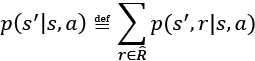
It can be computed as a marginal probability by taking the sum over all possible rewards:

This probability is called state-transition probability. Based on the state-transition probability, if the environment dynamics are deterministic, then it means that when the agent takes action at state , the transition to the next state, , will be 100 percent certain, that is, .

Visualization of a Markov process

A Markov process can be represented as a directed cyclic graph in which the nodes in the graph represent the different states of the environment. The edges of the graph (that is, the connections between the nodes) represent the transition probabilities between the states.

For example, let's consider a student deciding between three different situations: (A) studying for an exam at home, (B) playing video games at home, or (C) studying at the library. Furthermore, there is a terminal state (T) for going to sleep. The decisions are made every hour, and after making a decision, the student will remain in a chosen situation for that particular hour. Then, assume that when staying at home (state A), there is a 50 percent likelihood that the student switches the activity to playing video games. On the other hand, when the student is at state B (playing video games), there is a relatively high chance (80 percent) that the student will continue playing the video game in the subsequent hours.

The dynamics of the student's behavior is shown as a Markov process in the following figure, which includes a cyclic graph and a transition table:

The values on the edges of the graph represent the transition probabilities of the student's behavior, and their values are also shown in the table to the right. When considering the rows in the table, please note that the transition probabilities coming out of each state (node) always sum to 1.

Episodic versus continuing tasks

As the agent interacts with the environment, the sequence of observations or states forms a trajectory. There are two types of trajectories. If an agent's trajectory can be divided into subparts such that each starts at time t = 0 and ends in a terminal state (at t = T), the task is called an episodic task. On the other hand, if the trajectory is infinitely continuous without a terminal state, the task is called a continuing task.

The task related to a learning agent for the game of chess is an episodic task, whereas a cleaning robot that is keeping a house tidy is typically performing a continuing task. In this chapter, we only consider episodic tasks.

In episodic tasks, an episode is a sequence or trajectory that an agent takes from a starting state, , to a terminal state, :

For the Markov process shown in the previous figure, which depicts the task of a student studying for an exam, we may encounter episodes like the following three examples:

RL terminology: return, policy, and value function

Next, let's define some additional RL-specific terminology that we will need for the remainder of this chapter.

The return

The so-called return at time t is the cumulated reward obtained from the entire duration of an episode. Recall that is the immediate reward obtained after performing an action, , at time t; the subsequent rewards are , , and so forth.

The return at time t can then be calculated from the immediate reward as well as the subsequent ones, as follows:

Here, is the discount factor in range [0, 1]. The parameter indicates how much the future rewards are "worth" at the current moment (time t). Note that by setting , we would imply that we do not care about future rewards. In this case, the return will be equal to the immediate reward, ignoring the subsequent rewards after t + 1, and the agent will be short-sighted. On the other hand, if , the return will be the unweighted sum of all subsequent rewards.

Moreover, note that the equation for the return can be expressed in a simpler way using a recursion as follows:

This means that the return at time t is equal to the immediate reward r plus the discounted future-return at time t + 1. This is a very important property, which facilitates the computations of the return.

Let's compute the return at different time steps for the episodes in our previous student example. Assume , and that the only reward given is based on the result of the exam (+1 for passing the exam, and –1 for failing it). The rewards for intermediate time steps are 0.

:

• 
• 
• 
• ...
• 
• 

:

• 
• 
• ...
• 
• 

We leave the computation of the returns for the third episode as an exercise for the reader.

Policy

A policy typically denoted by is a function that determines the next action to take, which can be either deterministic, or stochastic (that is, the probability for taking the next action). A stochastic policy then has a probability distribution over actions that an agent can take at a given state:

During the learning process, the policy may change as the agent gains more experience. For example, the agent may start from a random policy, where the probability of all actions is uniform; meanwhile, the agent will hopefully learn to optimize its policy toward reaching the optimal policy. The optimal policy is the policy that yields the highest return.

Value function

The value function, also referred to as the state-value function, measures the goodness of each state—in other words, how good or bad it is to be in a particular state. Note that the criterion for goodness is based on the return.

Now, based on the return , we define the value function of state s as the expected return (the average return over all possible episodes) after following policy :

In an actual implementation, we usually estimate the value function using lookup tables, so we do not have to recompute it multiple times. (This is the dynamic programming aspect.) For example, in practice, when we estimate the value function using such tabular methods, we store all the state values in a table denoted by V(s). In a Python implementation, this could be a list or a NumPy array whose indexes refer to different states; or, it could be a Python dictionary, where the dictionary keys map the states to the respective values.

Moreover, we can also define a value for each state-action pair, which is called the action-value function and is denoted by . The action-value function refers to the expected return when the agent is at state and takes action . Extending the definition of state-value function to state-action pairs, we get the following:

Similar to referring to the optimal policy as , and also denote the optimal state-value and action-value functions.

Estimating the value function is an essential component of RL methods. We will cover different ways of calculating and estimating the state-value function and action-value function later in this chapter.

Before we move directly ahead into some RL algorithms, let's briefly go over the derivation for the Bellman equation, which we can use to implement the policy evaluation.

Dynamic programming using the Bellman equation

The Bellman equation is one of the central elements of many RL algorithms. The Bellman equation simplifies the computation of the value function, such that rather than summing over multiple time steps, it uses a recursion that is similar to the recursion for computing the return.

Based on the recursive equation for the total return , we can rewrite the value function as follows:

Notice that the immediate reward r is taken out of the expectation since it is a constant and known quantity at time t.

Similarly, for the action-value function, we could write:

We can use the environment dynamics to compute the expectation via summing over all probabilities of the next state and the corresponding rewards r:

Now, we can see that expectation of the return, , is essentially the state-value function . So, we can write as a function of :

This is called the Bellman equation, which relates the value function for a state, s, to the value function of its subsequent state, . This greatly simplifies the computation of the value function because it eliminates the iterative loop along the time axis.

Reinforcement learning algorithms

In this section, we will cover a series of learning algorithms. We will start with dynamic programming, which assumes that the transition dynamics (or the environment dynamics, that is, , are known. However, in most RL problems, this is not the case. To work around the unknown environment dynamics, RL techniques were developed that learn through interacting with the environment. These techniques include MC, TD learning, and the increasingly popular Q-learning and deep Q-learning approaches. The following figure describes the course of advancing RL algorithms, from dynamic programming to Q-learning:

In the following sections of this chapter, we will step through each of these RL algorithms. We will start with dynamic programming, before moving on to MC, and finally on to TD and its branches of on-policy SARSA (state–action–reward–state–action) and off-policy Q-learning. We will also move into deep Q-learning while we build some practical models.

Dynamic programming

In this section, we will focus on solving RL problems under the following assumptions:

• We have full knowledge about the environment dynamics; that is, all transition probabilities are known.
• The agent's state has the Markov property, which means that the next action and reward only depend on the current state and the choice of action we make at this moment or current time step.

The mathematical formulation for RL problems using a Markov decision process (MDP) was introduced earlier in this chapter. If you need a refresher, please refer to the section called The mathematical formulation of Markov decision processes, which introduced the formal definition of the value function following the policy , and the Bellman equation, which was derived using the environment dynamics.

We should emphasize that dynamic programming is not a practical approach for solving RL problems. The problem with using dynamic programming is that it assumes full knowledge of the environment dynamics, which is usually unreasonable or impractical for most real-world applications. However, from an educational standpoint, dynamic programming helps with introducing RL in a simple fashion and motivates the use of more advanced and complicated RL algorithms.

There are two main objectives via the tasks described in the following subsections:

1. Obtain the true state-value function, ; this task is also known as the prediction task and is accomplished with policy evaluation.
2. Find the optimal value function, , which is accomplished via generalized policy iteration.

Policy evaluation – predicting the value function with dynamic programming

Based on the Bellman equation, we can compute the value function for an arbitrary policy with dynamic programming when the environment dynamics are known. For computing this value function, we can adapt an iterative solution, where we start from , which is initialized to zero values for each state. Then, at each iteration i + 1, we update the values for each state based on the Bellman equation, which is, in turn, based on the values of states from a previous iteration i, as follows:

It can be shown that as the iterations increase to infinity, converges to the true state-value function .

Also, notice here that we do not need to interact with the environment. The reason for this is that we already know the environment dynamics accurately. As a result, we can leverage this information and estimate the value function easily.

After computing the value function, an obvious question is how that value function can be useful for us if our policy is still a random policy. The answer is that we can actually use this computed to improve our policy, as we will see next.

Improving the policy using the estimated value function

Now that we have computed the value function by following the existing policy, , we want to use and improve the existing policy, . This means that we want to find a new policy, , that for each state, s, following would yield higher or at least equal value than using the current policy, . In mathematical terms, we can express this objective for the improved policy, , as:

First, recall that a policy, , determines the probability of choosing each action, a, while the agent is at state s. Now, in order to find that always has a better or equal value for each state, we first compute the action-value function, , for each state, s, and action, a, based on the computed state value using the value function . We iterate through all the states, and for each state, s, we compare the value of the next state , that would occur if action a was selected.

After we have obtained the highest state value by evaluating all state-action pairs via , we can compare the corresponding action with the action selected by the current policy. If the action suggested by the current policy (that is, ) is different than the action suggested by the action-value function (that is, ), then we can update the policy by reassigning the probabilities of actions to match the action that gives the highest action value, . This is called the policy improvement algorithm.

Policy iteration

Using the policy improvement algorithm described in the previous subsection, it can be shown that the policy improvement will strictly yield a better policy, unless the current policy is already optimal (which means for each ). Therefore, if we iteratively perform policy evaluation followed by policy improvement, we are guaranteed to find the optimal policy.

Value iteration

We saw that by repeating the policy evaluation (compute and ) and policy improvement (finding such that ), we can reach the optimal policy. However, it can be more efficient if we combine the two tasks of policy evaluation and policy improvement into a single step. The following equation updates the value function for iteration i + 1 (denoted by ) based on the action that maximizes the weighted sum of the next state value and its immediate reward ():

In this case, the updated value for is maximized by choosing the best action out of all possible actions, whereas in policy evaluation, the updated value was using the weighted sum over all actions.

Reinforcement learning with Monte Carlo

As we saw in the previous section on dynamic programming, it relies on a simplistic assumption that the environment's dynamics are fully known. Moving away from the dynamic programming approach, we now assume that we do not have any knowledge about the environment dynamics.

That is, we do not know the state-transition probabilities of the environment, and instead, we want the agent to learn through interacting with the environment. Using MC methods, the learning process is based on the so-called simulated experience.

For MC-based RL, we define an agent class that follows a probabilistic policy, , and based on this policy, our agent takes an action at each step. This results in a simulated episode.

Earlier, we defined the state-value function, such that the value of a state indicates the expected return from that state. In dynamic programming, this computation relied on the knowledge of the environment dynamics, that is, .

However, from now on, we will develop algorithms that do not require the environment dynamics. MC-based methods solve this problem by generating simulated episodes where an agent interacts with the environment. From these simulated episodes, we will be able to compute the average return for each state visited in that simulated episode.

State-value function estimation using MC

After generating a set of episodes, for each state, s, the set of episodes that all pass through state s is considered for calculating the value of state s. Let's assume that a lookup table is used for obtaining the value corresponding to the value function, . MC updates for estimating the value function are based on the total return obtained in that episode starting from the first time that state s is visited. This algorithm is called first-visit Monte Carlo value prediction.

Action-value function estimation using MC

When the environment dynamics are known, we can easily infer the action-value function from a state-value function by looking one step ahead to find the action that gives the maximum value, as was shown in the Dynamic programming section. However, this is not feasible if the environment dynamics are unknown.

To solve this issue, we can extend the algorithm for estimating the first-visit MC state-value prediction. For instance, we can compute the estimated return for each state-action pair using the action-value function. To obtain this estimated return, we consider visits to each state-action pair (s, a), which refers to visiting state s and taking action a.

However, a problem arises since some actions may never be selected, resulting in insufficient exploration. There are a few ways to resolve this. The simplest approach is called exploratory start, which assumes that every state-action pair has a non zero probability at the beginning of the episode.

Another approach to deal with this lack-of-exploration issue is called -greedy policy, which will be discussed in the next section on policy improvement.

Finding an optimal policy using MC control

MC control refers to the optimization procedure for improving a policy. Similar to the policy iteration approach in previous section (Dynamic programming), we can repeatedly alternate between policy evaluation and policy improvement until we reach the optimal policy. So, starting from a random policy, , the process of alternating between policy evaluation and policy improvement can be illustrated as follows:

Policy improvement – computing the greedy policy from the action-value function

Given an action-value function, q(s, a), we can generate a greedy (deterministic) policy as follows:

In order to avoid the lack-of-exploration problem, and to consider the non-visited state-action pairs as discussed earlier, we can let the non-optimal actions have a small chance () to be chosen. This is called the -greedy policy, according to which, all non-optimal actions at state s have a minimal probability of being selected (instead of 0), and the optimal action has a probability of (instead of 1).

Temporal difference learning

So far, we have seen two fundamental RL techniques, dynamic programming and MC-based learning. Recall that dynamic programming relies on the complete and accurate knowledge of the environment dynamics. The MC-based method, on the other hand, learns by simulated experience. In this section, we will now introduce a third RL method called TD learning, which can be considered as an improvement or extension of the MC-based RL approach.

Similar to the MC technique, TD learning is also based on learning by experience and, therefore, does not require any knowledge of environment dynamics and transition probabilities. The main difference between the TD and MC techniques is that in MC, we have to wait until the end of the episode to be able to calculate the total return.

However, in TD learning, we can leverage some of the learned properties to update the estimated values before reaching the end of the episode. This is called bootstrapping (in the context of RL, the term bootstrapping is not to be confused with the bootstrap estimates we used in Chapter 7, Combining Different Models for Ensemble Learning).

Similar to the dynamic programming approach and MC-based learning, we will consider two tasks: estimating the value function (which is also called value prediction) and improving the policy (which is also called the control task).

TD prediction

Let's first revisit the value prediction by MC. At the end of each episode, we are able to estimate the return for each time step t. Therefore, we can update our estimates for the visited states as follows:

Here, is used as the target return to update the estimated values, and is a correction term added to our current estimate of the value . The value is a hyperparameter denoting the learning rate, which is kept constant during learning.

Notice that in MC, the correction term uses the actual return, , which is not known until the end of the episode. To clarify this, we can rename the actual return, , to , where the subscript indicates that this is the return obtained at time step t while considering all the events occurred from time step t until the final time step, T.

In TD learning, we replace the actual return, , with a new target return, , which significantly simplifies the updates for the value function, . The update-formula based on TD learning is as follows:

Here, the target return, , is using the observed reward, , and estimated value of the next immediate step. Notice the difference between MC and TD. In MC, is not available until the end of the episode, so we should execute as many steps as needed to get there. On the contrary, in TD, we only need to go one step ahead to get the target return. This is also known as TD(0).

Furthermore, the TD(0) algorithm can be generalized to the so-called n-step TD algorithm, which incorporates more future steps – more precisely, the weighted sum of n future steps. If we define n = 1, then the n-step TD procedure is identical to TD(0), which was described in the previous paragraph. If , however, the n-step TD algorithm will be the same as the MC algorithm. The update-rule for n-step TD is as follows:

And is defined as:

Now that we have covered the prediction task using the TD algorithm, we can move on to the control task. We will cover two algorithms for TD control: an on-policy control and an off-policy control. In both cases, we use the GPI that was used in both the dynamic programming and MC algorithms. In on-policy TD control, the value function is updated based on the actions from the same policy that the agent is following, while in an off-policy algorithm, the value function is updated based on actions outside the current policy.

On-policy TD control (SARSA)

For simplicity, we only consider the one-step TD algorithm, or TD(0). However, the on-policy TD control algorithm can be readily generalized to n-step TD. We will start by extending the prediction formula for defining the state-value function to describe the action-value function. To do this, we use a lookup table, that is, a tabular 2D-array, , which represents the action-value function for each state-action pair. In this case, we will have the following:

This algorithm is often called SARSA, referring to the quintuple that is used in the update formula.

As we saw in the previous sections describing the dynamic programming and MC algorithms, we can use the GPI framework, and starting from the random policy, we can repeatedly estimate the action-value function for the current policy and then optimize the policy using the -greedy policy based on the current action-value function.

Off-policy TD control (Q-learning)

We saw when using the previous on-policy TD control algorithm that how we estimate the action-value function is based on the policy that is used in the simulated episode. After updating the action-value function, a separate step for policy improvement is performed by taking the action that has the higher value.

An alternative (and better) approach is to combine these two steps. In other words, imagine the agent is following policy , generating an episode with the current transition quintuple . Instead of updating the action-value function using the action value of that is taken by the agent, we can find the best action even if it is not actually chosen by the agent following the current policy. (That's why this is considered an off-policy algorithm.)

To do this, we can modify the update rule to consider the maximum Q-value by varying different actions in the next immediate state. The modified equation for updating the Q-values is as follows:

We encourage you to compare the update rule here with that of the SARSA algorithm. As you can see, we find the best action in the next state, , and use that in the correction term to update our estimate of .

To put these materials into perspective, in the next section, we will see how to implement the Q-learning algorithm for solving the grid world problem.

Implementing our first RL algorithm

In this section, we will cover the implementation of the Q-learning algorithm to solve the grid world problem. To do this, we use the OpenAI Gym toolkit.

Introducing the OpenAI Gym toolkit

OpenAI Gym is a specialized toolkit for facilitating the development of RL models. OpenAI Gym comes with several predefined environments. Some basic examples are CartPole and MountainCar, where the tasks are to balance a pole and to move a car up a hill, respectively, as the names suggest. There are also many advanced robotics environments for training a robot to fetch, push, and reach for items on a bench or training a robotic hand to orient blocks, balls, or pens. Moreover, OpenAI Gym provides a convenient, unified framework for developing new environments. More information can be found on its official website: https://gym.openai.com/.

To follow the OpenAI Gym code examples in the next sections, you need to install the gym library, which can be easily done using pip:

> pip install gym

If you need additional help with the installation, please see the official installation guide at https://gym.openai.com/docs/#installation.

Working with the existing environments in OpenAI Gym

For practice with the Gym environments, let's create an environment from CartPole-v1, which already exists in OpenAI Gym. In this example environment, there is a pole attached to a cart that can move horizontally, as shown in the next figure:

The movements of the pole are governed by the laws of physics, and the goal for RL agents is to learn how to move the cart to stabilize the pole and prevent it from tipping over to either side.

Now, let's look at some properties of the CartPole environment in the context of RL, such as its state (or observation) space, action space, and how to execute an action:

>>> import gym
>>> env = gym.make('CartPole-v1')
>>> env.observation_space
Box(4,)
>>> env.action_space
Discrete(2)

In the preceding code, we created an environment for the CartPole problem. The observation space for this environment is Box(4,), which represents a four-dimensional space corresponding to four real-valued numbers: the position of the cart, the cart's velocity, the angle of the pole, and the velocity of the tip of the pole. The action space is a discrete space, Discrete(2), with two choices: pushing the cart either to the left or to the right.

The environment object, env, that we previously created by calling gym.make('CartPole-v1') has a reset() method that we can use to reinitialize an environment prior to each episode. Calling the reset() method will basically set the pole's starting state ():

>>> env.reset()
array([-0.03908273, -0.00837535,  0.03277162, -0.0207195 ])

The values in the array returned by the env.reset() method call mean that the initial position of the cart is –0.039 with velocity –0.008, and the angle of the pole is 0.033 radian while the angular velocity of its tip is –0.021. Upon calling the reset() method, these values are initialized with random values with uniform distribution in the range [–0.05, 0.05].

After resetting the environment, we can interact with the environment by choosing an action and executing it by passing the action to the step() method:

>>> env.step(action=0)
(array([-0.03925023, -0.20395158,  0.03235723,  0.28212046]), 1.0, False, {})
>>> env.step(action=1)
(array([-0.04332927, -0.00930575,  0.03799964, -0.00018409]), 1.0, False, {})

Via the previous two commands, env.step(action=0) and env.step(action=1), we pushed the cart to the left (action=0) and then to the right (action=1), respectively. Based on the selected action, the cart and its pole can move as governed by the laws of physics. Every time we call env.step(), it returns a tuple consisting of four elements:

• An array for the new state (or observations)
• A reward (a scalar value of type float)
• A termination flag (True or False)
• A Python dictionary containing auxiliary information

The env object also has a render() method, which we can execute after each step (or a series of steps) to visualize the environment and the movements of the pole and cart, through time.

The episode terminates when the angle of the pole becomes larger than 12 degrees (from either side) with respect to an imaginary vertical axis, or when the position of the cart is more than 2.4 units from the center position. The reward defined in this example is to maximize the time the cart and pole are stabilized within the valid regions—in other words, the total reward (that is, return) can be maximized by maximizing the length of the episode.

A grid world example

After introducing the CartPole environment as a warm-up exercise for working with the OpenAI Gym toolkit, we will now switch to a different environment. We will work with a grid world example, which is a simplistic environment with m rows and n columns. Considering m = 4 and n = 6, we can summarize this environment as shown in the following figure:

In this environment, there are 30 different possible states. Four of these states are terminal states: a pot of gold at state 16 and three traps at states 10, 15, and 22. Landing in any of these four terminal states will end the episode, but with a difference between the gold and trap states. Landing on the gold state yields a positive reward, +1, whereas moving the agent onto one of the trap states yields a negative reward, –1. All other states have a reward of 0. The agent always starts from state 0. Therefore, every time we reset the environment, the agent will go back to state 0. The action space consists of four directions: move up, down, left, and right.

When the agent is at the outer boundary of the grid, selecting an action that would result in leaving the grid will not change the state.

Next, we will see how to implement this environment in Python, using the OpenAI Gym package.

Implementing the grid world environment in OpenAI Gym

For experimenting with the grid world environment via OpenAI Gym, using a script editor or IDE rather than executing the code interactively is highly recommended.

First, we create a new Python script named gridworld_env.py and then proceed by importing the necessary packages and two helper functions that we define for building the visualization of the environment.

In order to render the environments for visualization purposes, OpenAI Gym library uses the Pyglet library and provides wrapper classes and functions for our convenience. We will use these wrapper classes for visualizing the grid world environment in the following code example. More details about these wrapper classes can be found at

https://github.com/openai/gym/blob/master/gym/envs/classic_control/rendering.py

The following code example uses those wrapper classes:

## Script: gridworld_env.py
import numpy as np
from gym.envs.toy_text import discrete
from collections import defaultdict
import time
import pickle
import os
from gym.envs.classic_control import rendering
CELL_SIZE = 100
MARGIN = 10
def get_coords(row, col, loc='center'):
    xc = (col+1.5) * CELL_SIZE
    yc = (row+1.5) * CELL_SIZE
    if loc == 'center':
        return xc, yc
    elif loc == 'interior_corners':
        half_size = CELL_SIZE//2 - MARGIN
        xl, xr = xc - half_size, xc + half_size
        yt, yb = xc - half_size, xc + half_size
        return [(xl, yt), (xr, yt), (xr, yb), (xl, yb)]
    elif loc == 'interior_triangle':
        x1, y1 = xc, yc + CELL_SIZE//3
        x2, y2 = xc + CELL_SIZE//3, yc - CELL_SIZE//3
        x3, y3 = xc - CELL_SIZE//3, yc - CELL_SIZE//3
        return [(x1, y1), (x2, y2), (x3, y3)]
def draw_object(coords_list):
    if len(coords_list) == 1: # -> circle
        obj = rendering.make_circle(int(0.45*CELL_SIZE))
        obj_transform = rendering.Transform()
        obj.add_attr(obj_transform)
        obj_transform.set_translation(*coords_list[0])
        obj.set_color(0.2, 0.2, 0.2) # -> black
    elif len(coords_list) == 3: # -> triangle
        obj = rendering.FilledPolygon(coords_list)
        obj.set_color(0.9, 0.6, 0.2) # -> yellow
    elif len(coords_list) > 3: # -> polygon
        obj = rendering.FilledPolygon(coords_list)
        obj.set_color(0.4, 0.4, 0.8) # -> blue
    return obj

The first helper function, get_coords(), returns the coordinates of the geometric shapes that we will use to annotate the grid world environment, such as a triangle to display the gold or circles to display the traps. The list of coordinates is passed to draw_object(), which decides to draw a circle, a triangle, or a polygon based on the length of the input list of coordinates.

Now, we can define the grid world environment. In the same file (gridworld_env.py), we define a class named GridWorldEnv, which inherits from OpenAI Gym's DiscreteEnv class. The most important function of this class is the constructor method, __init__(), where we define the action space, specify the role of each action, and determine the terminal states (gold as well as traps) as follows:

class GridWorldEnv(discrete.DiscreteEnv):
    def __init__(self, num_rows=4, num_cols=6, delay=0.05):
        self.num_rows = num_rows
        self.num_cols = num_cols
        self.delay = delay
        move_up = lambda row, col: (max(row-1, 0), col)
        move_down = lambda row, col: (min(row+1, num_rows-1), col)
        move_left = lambda row, col: (row, max(col-1, 0))
        move_right = lambda row, col: (
            row, min(col+1, num_cols-1))
        self.action_defs={0: move_up, 1: move_right,
                          2: move_down, 3: move_left}
        ## Number of states/actions
        nS = num_cols*num_rows
        nA = len(self.action_defs)
        self.grid2state_dict={(s//num_cols, s%num_cols):s
                              for s in range(nS)}
        self.state2grid_dict={s:(s//num_cols, s%num_cols)
                              for s in range(nS)}
        ## Gold state
        gold_cell = (num_rows//2, num_cols-2)
        
        ## Trap states
        trap_cells = [((gold_cell[0]+1), gold_cell[1]),
                       (gold_cell[0], gold_cell[1]-1),
                       ((gold_cell[0]-1), gold_cell[1])]
        gold_state = self.grid2state_dict[gold_cell]
        trap_states = [self.grid2state_dict[(r, c)]
                       for (r, c) in trap_cells]
        self.terminal_states = [gold_state] + trap_states
        print(self.terminal_states)
        ## Build the transition probability
        P = defaultdict(dict)
        for s in range(nS):
            row, col = self.state2grid_dict[s]
            P[s] = defaultdict(list)
            for a in range(nA):
                action = self.action_defs[a]
                next_s = self.grid2state_dict[action(row, col)]
                
                ## Terminal state
                if self.is_terminal(next_s):
                    r = (1.0 if next_s == self.terminal_states[0]
                         else -1.0)
                else:
                    r = 0.0
                if self.is_terminal(s):
                    done = True
                    next_s = s
                else:
                    done = False
                P[s][a] = [(1.0, next_s, r, done)]
        ## Initial state distribution
        isd = np.zeros(nS)
        isd[0] = 1.0
        super(GridWorldEnv, self).__init__(nS, nA, P, isd)
        self.viewer = None
        self._build_display(gold_cell, trap_cells)
    def is_terminal(self, state):
        return state in self.terminal_states
    def _build_display(self, gold_cell, trap_cells):
        screen_width = (self.num_cols+2) * CELL_SIZE
        screen_height = (self.num_rows+2) * CELL_SIZE
        self.viewer = rendering.Viewer(screen_width, 
                                       screen_height)
        all_objects = []
        ## List of border points' coordinates
        bp_list = [
            (CELL_SIZE-MARGIN, CELL_SIZE-MARGIN),
            (screen_width-CELL_SIZE+MARGIN, CELL_SIZE-MARGIN),
            (screen_width-CELL_SIZE+MARGIN,
             screen_height-CELL_SIZE+MARGIN),
            (CELL_SIZE-MARGIN, screen_height-CELL_SIZE+MARGIN)
        ]
        border = rendering.PolyLine(bp_list, True)
        border.set_linewidth(5)
        all_objects.append(border)
        ## Vertical lines
        for col in range(self.num_cols+1):
            x1, y1 = (col+1)*CELL_SIZE, CELL_SIZE
            x2, y2 = (col+1)*CELL_SIZE,
                     (self.num_rows+1)*CELL_SIZE
            line = rendering.PolyLine([(x1, y1), (x2, y2)], False)
            all_objects.append(line)
        
        ## Horizontal lines
        for row in range(self.num_rows+1):
            x1, y1 = CELL_SIZE, (row+1)*CELL_SIZE
            x2, y2 = (self.num_cols+1)*CELL_SIZE,
                     (row+1)*CELL_SIZE
            line=rendering.PolyLine([(x1, y1), (x2, y2)], False)
            all_objects.append(line)
        
        ## Traps: --> circles
        for cell in trap_cells:
            trap_coords = get_coords(*cell, loc='center')
            all_objects.append(draw_object([trap_coords]))
        
        ## Gold:  --> triangle
        gold_coords = get_coords(*gold_cell,
                                 loc='interior_triangle')
        all_objects.append(draw_object(gold_coords))
        ## Agent --> square or robot
        if (os.path.exists('robot-coordinates.pkl') and
                CELL_SIZE==100):
            agent_coords = pickle.load(
                open('robot-coordinates.pkl', 'rb'))
            starting_coords = get_coords(0, 0, loc='center')
            agent_coords += np.array(starting_coords)
        else:
            agent_coords = get_coords(
                0, 0, loc='interior_corners')
        agent = draw_object(agent_coords)
        self.agent_trans = rendering.Transform()
        agent.add_attr(self.agent_trans)
        all_objects.append(agent)
        for obj in all_objects:
            self.viewer.add_geom(obj)
    def render(self, mode='human', done=False):
        if done:
            sleep_time = 1
        else:
            sleep_time = self.delay
        x_coord = self.s % self.num_cols
        y_coord = self.s // self.num_cols
        x_coord = (x_coord+0) * CELL_SIZE
        y_coord = (y_coord+0) * CELL_SIZE
        self.agent_trans.set_translation(x_coord, y_coord)
        rend = self.viewer.render(
             return_rgb_array=(mode=='rgb_array'))
        time.sleep(sleep_time)
        return rend
    def close(self):
        if self.viewer:
            self.viewer.close()
            self.viewer = None

This code implements the grid world environment, from which we can create instances of this environment. We can then interact with it in a manner similar to that in the CartPole example. The implemented class, GridWorldEnv, inherits methods such as reset() for resetting the state and step() for executing an action. The details of the implementation are as follows:

• We defined the four different actions using lambda functions: move_up(), move_down(), move_left(), and move_right().
• The NumPy array isd holds the probabilities of the starting states so that a random state will be selected based on this distribution when the reset() method (from the parent class) is called. Since we always start from state 0 (the lower-left corner of the grid world), we set the probability of state 0 to 1.0 and the probabilities of all other 29 states to 0.0.
• The transition probabilities, defined in the Python dictionary P, determine the probabilities of moving from one state to another state when an action is selected. This allows us to have a probabilistic environment where taking an action could have different outcomes based on the stochasticity of the environment. For simplicity, we just use a single outcome, which is to change the state in the direction of the selected action. Finally, these transition probabilities will be used by the env.step() function to determine the next state.
• Furthermore, the function _build_display() will set up the initial visualization of the environment, and the render() function will show the movements of the agent.

Now, we can test this implementation by creating a new environment and visualize a random episode by taking random actions at each state. Include the following code at the end of the same Python script (gridworld_env.py) and then execute the script:

if __name__ == '__main__':
    env = GridWorldEnv(5, 6)
    for i in range(1):
        s = env.reset()
        env.render(mode='human', done=False)
        while True:
            action = np.random.choice(env.nA)
            res = env.step(action)
            print('Action  ', env.s, action, ' -> ', res)
            env.render(mode='human', done=res[2])
            if res[2]:
                break
    env.close()

After executing the script, you should see a visualization of the grid world environment as depicted in the following figure:

Solving the grid world problem with Q-learning

After focusing on the theory and the development process of RL algorithms, as well as setting up the environment via the OpenAI Gym toolkit, we will now implement the currently most popular RL algorithm, Q-learning. For this, we will use the grid world example that we already implemented in the script gridworld_env.py.

Implementing the Q-learning algorithm

Now, we create a new script and name it agent.py. In this agent.py script, we define an agent for interacting with the environment as follows:

## Script: agent.py
from collections import defaultdict
import numpy as np
class Agent(object):
    def __init__(
            self, env,
            learning_rate=0.01,
            discount_factor=0.9,
            epsilon_greedy=0.9,
            epsilon_min=0.1,
            epsilon_decay=0.95):
        self.env = env
        self.lr = learning_rate
        self.gamma = discount_factor
        self.epsilon = epsilon_greedy
        self.epsilon_min = epsilon_min
        self.epsilon_decay = epsilon_decay
        ## Define the q_table
        self.q_table = defaultdict(lambda: np.zeros(self.env.nA))
    def choose_action(self, state):
        if np.random.uniform() < self.epsilon:
            action = np.random.choice(self.env.nA)
        else:
            q_vals = self.q_table[state]
            perm_actions = np.random.permutation(self.env.nA)
            q_vals = [q_vals[a] for a in perm_actions]
            perm_q_argmax = np.argmax(q_vals)
            action = perm_actions[perm_q_argmax]
        return action
    def _learn(self, transition):
        s, a, r, next_s, done = transition
        q_val = self.q_table[s][a]
        if done:
            q_target = r
        else:
            q_target = r + self.gamma*np.max(self.q_table[next_s])
        ## Update the q_table
        self.q_table[s][a] += self.lr * (q_target - q_val)
        ## Adjust the epislon
        self._adjust_epsilon()
    def _adjust_epsilon(self):
        if self.epsilon > self.epsilon_min:
            self.epsilon *= self.epsilon_decay

The __init__() constructor sets up various hyperparameters such as the learning rate, discount factor (), and the parameters for the -greedy policy. Initially, we start with a high value of , but the method _adjust_epsilon() reduces it until it reaches the minimum value, . The method choose_action() chooses an action based on the -greedy policy as follows. A random uniform number is selected to determine whether the action should be selected randomly or otherwise, based on the action-value function. The method _learn() implements the update rule for the Q-learning algorithm. It receives a tuple for each transition, which consists of the current state (s), selected action (a), observed reward (r), next state (s'), as well as a flag to determine whether the end of the episode has been reached or not. The target value is equal to the observed reward (r) if this is flagged as end-of-episode; otherwise, the target is .

Finally, for our next step, we create a new script, qlearning.py, to put everything together and train the agent using the Q-learning algorithm.

In the following code, we define a function, run_qlearning(), that implements the Q-learning algorithm, simulating an episode by calling the _choose_action() method of the agent and executing the environment. Then, the transition tuple is passed to the _learn() method of the agent to update the action-value function. In addition, for monitoring the learning process, we also store the final reward of each episode (which could be –1 or +1), as well as the length of episodes (the number of moves taken by the agent from the start of the episode until the end).

The list of rewards and the number of moves is then plotted using the function plot_learning_history():

## Script: qlearning.py
from gridworld_env import GridWorldEnv
from agent import Agent
from collections import namedtuple
import matplotlib.pyplot as plt
import numpy as np
np.random.seed(1)
Transition = namedtuple(
    'Transition', ('state', 'action', 'reward',
                   'next_state', 'done'))
def run_qlearning(agent, env, num_episodes=50):
    history = []
    for episode in range(num_episodes):
        state = env.reset()
        env.render(mode='human')
        final_reward, n_moves = 0.0, 0
        while True:
            action = agent.choose_action(state)
            next_s, reward, done, _ = env.step(action)
            agent._learn(Transition(state, action, reward,
                                    next_s, done))
            env.render(mode='human', done=done)
            state = next_s
            n_moves += 1
            if done:
                break
            final_reward = reward
        history.append((n_moves, final_reward))
        print('Episode %d: Reward %.1f #Moves %d'
              % (episode, final_reward, n_moves))
    return history
def plot_learning_history(history):
    fig = plt.figure(1, figsize=(14, 10))
    ax = fig.add_subplot(2, 1, 1)
    episodes = np.arange(len(history))
    moves = np.array([h[0] for h in history])
    plt.plot(episodes, moves, lw=4,
             marker='o', markersize=10)
    ax.tick_params(axis='both', which='major', labelsize=15)
    plt.xlabel('Episodes', size=20)
    plt.ylabel('# moves', size=20)
    ax = fig.add_subplot(2, 1, 2)
    rewards = np.array([h[1] for h in history])
    plt.step(episodes, rewards, lw=4)
    ax.tick_params(axis='both', which='major', labelsize=15)
    plt.xlabel('Episodes', size=20)
    plt.ylabel('Final rewards', size=20)
    plt.savefig('q-learning-history.png', dpi=300)
    plt.show()
if __name__ == '__main__':
    env = GridWorldEnv(num_rows=5, num_cols=6)
    agent = Agent(env)
    history = run_qlearning(agent, env)
    env.close()
    plot_learning_history(history)

Executing this script will run the Q-learning program for 50 episodes. The behavior of the agent will be visualized, and you can see that at the beginning of the learning process, the agent mostly ends up in the trap states. But through time, it learns from its failures and eventually finds the gold state (for instance, the first time in episode 7). The following figure shows the agent's number of moves and rewards:

The plotted learning history shown in the previous figure indicates that the agent, after 30 episodes, learns a short path to get to the gold state. As a result, the lengths of the episodes after the 30th episode are more or less the same, with minor deviations due to the -greedy policy.

A glance at deep Q-learning

In the previous code, we saw an implementation of the popular Q-learning algorithm for the grid world example. This example consisted of a discrete state space of size 30, where it was sufficient to store the Q-values in a Python dictionary.

However, we should note that sometimes the number of states can get very large, possibly almost infinitely large. Also, we may be dealing with a continuous state space instead of working with discrete states. Moreover, some states may not be visited at all during training, which can be problematic when generalizing the agent to deal with such unseen states later.

To address these problems, instead of representing the value function in a tabular format like , or , for the action-value function, we use a function approximation approach. Here, we define a parametric function, , that can learn to approximate the true value function, that is, , where is a set of input features (or "featurized" states).

When the approximator function, , is a deep neural network (DNN), the resulting model is called a deep Q-network (DQN). For training a DQN model, the weights are updated according to the Q-learning algorithm. An example of a DQN model is shown in the following figure, where the states are represented as features passed to the first layer:

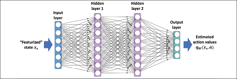
Now, let's see how we can train a DQN using the deep Q-learning algorithm. Overall, the main approach is very similar to the tabular Q-learning method. The main difference is that we now have a multilayer NN that computes the action values.

Training a DQN model according to the Q-learning algorithm

In this section, we describe the procedure for training a DQN model using the Q-learning algorithm. The deep Q-learning approach requires us to make some modifications to our previously implemented standard Q-learning approach.

One such modification is in the agent's choose_action() method, which in the code of the previous section for Q-learning was simply accessing the action values stored in a dictionary. Now this function should be changed to perform a forward pass of the NN model for computing the action values.

The other modifications needed for the deep Q-learning algorithm are described in the following two subsections.

Replay memory

Using the previous tabular method for Q-learning, we could update the values for specific state-action pairs without affecting the values of others. However, now that we approximate q(s, a) with an NN model, updating the weights for a state-action pair will likely affect the output of other states as well. When training NNs using stochastic gradient descent for a supervised task (for example, a classification task), we use multiple epochs to iterate through the training data multiple times until it converges.

This is not feasible in Q-learning, since the episodes will change during the training and as a result, some states that were visited in the early stages of training will become less likely to be visited later.

Furthermore, another problem is that when we train an NN, we assume that the training examples are IID (independent and identically distributed). However, the samples taken from an episode of the agent are not IID, as they obviously form a sequence of transitions.

To solve these issues, as the agent interacts with the environment and generates a transition quintuple , we store a large (but finite) number of such transitions in a memory buffer, often called replay memory. After each new interaction (that is, the agent selects an action and executes it in the environment), the resulting new transition quintuple is appended to the memory.

To keep the size of the memory bounded, the oldest transition will be removed from the memory (for example, if it is a Python list, we can use the pop(0) method to remove the first element of the list). Then, a mini-batch of examples is randomly selected from the memory buffer, which will be used for computing the loss and updating the network parameters. The following figure illustrates the process:

Determining the target values for computing the loss

Another required change from the tabular Q-learning method is how to adapt the update rule for training the DQN model parameters. Recall that a transition quintuple, T, stored in the batch of examples, contains .

As shown in the following figure, we perform two forward passes of the DQN model. The first forward pass uses the features of the current state (). Then, the second forward pass uses the features of the next state (). As a result, we will obtain the estimated action values, and , from the first and second forward pass, respectively. (Here, this notation means a vector of Q-values for all actions in .) From the transition quintuple, we know that action a is selected by the agent.

Therefore, according to the Q-learning algorithm, we need to update the action value corresponding to the state-action pair with the scalar target value . Instead of forming a scalar target value, we will create a target action-value vector that retains the action values for other actions, , as shown in the following figure:

We treat this as a regression problem, using the following three quantities:

• The currently predicted values,
• The target value vector as described
• The standard mean squared error (MSE) cost function

As a result, the losses will be zero for every action except for a. Finally, the computed loss will be backpropagated to update the network parameters.

Implementing a deep Q-learning algorithm

Finally, we will use all these techniques for implementing a deep Q-learning algorithm. This time, we use the CartPole environment from the OpenAI gym environment that we introduced earlier. Recall that the CartPole environment has a continuous state space of size 4. In the following code, we define a class, DQNAgent, that builds the model and specifies various hyperparameters.

This class has two additional methods compared to the previous agent that was based on tabular Q-learning. The method remember() will append a new transition quintuple to the memory buffer, and the method replay() will create a mini-batch of example transitions and pass that to the _learn() method for updating the network's weight parameters:

import gym
import numpy as np
import tensorflow as tf
import random
import matplotlib.pyplot as plt
from collections import namedtuple
from collections import deque
np.random.seed(1)
tf.random.set_seed(1)
Transition = namedtuple(
            'Transition', ('state', 'action', 'reward',
                           'next_state', 'done'))
class DQNAgent:
    def __init__(
            self, env, discount_factor=0.95,
            epsilon_greedy=1.0, epsilon_min=0.01,
            epsilon_decay=0.995, learning_rate=1e-3,
            max_memory_size=2000):
        self.enf = env
        self.state_size = env.observation_space.shape[0]
        self.action_size = env.action_space.n
        self.memory = deque(maxlen=max_memory_size)
        self.gamma = discount_factor
        self.epsilon = epsilon_greedy
        self.epsilon_min = epsilon_min
        self.epsilon_decay = epsilon_decay
        self.lr = learning_rate
        self._build_nn_model()
    def _build_nn_model(self, n_layers=3):
        self.model = tf.keras.Sequential()
        
        ## Hidden layers
        for n in range(n_layers-1):
            self.model.add(tf.keras.layers.Dense(
                units=32, activation='relu'))
            self.model.add(tf.keras.layers.Dense(
                units=32, activation='relu'))
        ## Last layer
        self.model.add(tf.keras.layers.Dense(
            units=self.action_size))
        ## Build & compile model
        self.model.build(input_shape=(None, self.state_size))
        self.model.compile(
            loss='mse',
            optimizer=tf.keras.optimizers.Adam(lr=self.lr))
    def remember(self, transition):
        self.memory.append(transition)
    def choose_action(self, state):
        if np.random.rand() <= self.epsilon:
            return random.randrange(self.action_size)
        q_values = self.model.predict(state)[0]
        return np.argmax(q_values)  # returns action
    def _learn(self, batch_samples):
        batch_states, batch_targets = [], []
        for transition in batch_samples:
            s, a, r, next_s, done = transition
            if done:
                target = r
            else:
                target = (r +
                    self.gamma * np.amax(
                        self.model.predict(next_s)[0]
                    )
                )
            target_all = self.model.predict(s)[0]
            target_all[a] = target
            batch_states.append(s.flatten())
            batch_targets.append(target_all)
            self._adjust_epsilon()
        return self.model.fit(x=np.array(batch_states),
                              y=np.array(batch_targets),
                              epochs=1,
                              verbose=0)
    def _adjust_epsilon(self):
        if self.epsilon > self.epsilon_min:
            self.epsilon *= self.epsilon_decay
    def replay(self, batch_size):
        samples = random.sample(self.memory, batch_size)
        history = self._learn(samples)
        return history.history['loss'][0]

Finally, with the following code, we train the model for 200 episodes, and at the end visualize the learning history using the function plot_learning_history():

def plot_learning_history(history):
    fig = plt.figure(1, figsize=(14, 5))
    ax = fig.add_subplot(1, 1, 1)
    episodes = np.arange(len(history[0]))+1
    plt.plot(episodes, history[0], lw=4,
             marker='o', markersize=10)
    ax.tick_params(axis='both', which='major', labelsize=15)
    plt.xlabel('Episodes', size=20)
    plt.ylabel('# Total Rewards', size=20)
    plt.show()
## General settings
EPISODES = 200
batch_size = 32
init_replay_memory_size = 500
if __name__ == '__main__':
    env = gym.make('CartPole-v1')
    agent = DQNAgent(env)
    state = env.reset()
    state = np.reshape(state, [1, agent.state_size])
    ## Filling up the replay-memory
    for i in range(init_replay_memory_size):
        action = agent.choose_action(state)
        next_state, reward, done, _ = env.step(action)
        next_state = np.reshape(next_state, [1, agent.state_size])
        agent.remember(Transition(state, action, reward,
                                  next_state, done))
        if done:
            state = env.reset()
            state = np.reshape(state, [1, agent.state_size])
        else:
            state = next_state
    total_rewards, losses = [], []
    for e in range(EPISODES):
        state = env.reset()
        if e % 10 == 0:
            env.render()
        state = np.reshape(state, [1, agent.state_size])
        for i in range(500):
            action = agent.choose_action(state)
            next_state, reward, done, _ = env.step(action)
            next_state = np.reshape(next_state,
                                    [1, agent.state_size])
            agent.remember(Transition(state, action, reward,
                                      next_state, done))
            state = next_state
            if e % 10 == 0:
                env.render()
            if done:
                total_rewards.append(i)
                print('Episode: %d/%d, Total reward: %d'
                      % (e, EPISODES, i))
                break
            loss = agent.replay(batch_size)
            losses.append(loss)
    plot_learning_history(total_rewards)

After training the agent for 200 episodes, we see that it indeed learned to increase the total rewards over time, as shown in the following plot:

Note that the total rewards obtained in an episode is equal to the amount of time that the agent is able to balance the pole. The learning history plotted in this figure shows that after about 30 episodes, the agent learns how to balance the pole and hold it for more than 200 time steps.

Chapter and book summary

In this chapter, we covered the essential concepts in RL, starting from the very foundations, and how RL can support decision making in complex environments.

We learned about agent-environment interactions and Markov decision processes (MDP), and we considered three main approaches for solving RL problems: dynamic programming, MC learning, and TD learning. We discussed that the dynamic programming algorithm assumes that the full knowledge of environment dynamics is available, an assumption that is not typically true for most real-world problems.

Then, we saw how the MC- and TD-based algorithms learn by allowing an agent to interact with the environment and generate a simulated experience. After discussing the underlying theory, we implemented the Q-learning algorithm as an off-policy subcategory of the TD algorithm for solving the grid world example. Finally, we covered the concept of function approximation and deep Q-learning in particular, which can be used for problems with large or continuous state spaces.

We hope you enjoyed this last chapter of Python Machine Learning and our exciting tour of machine learning and deep learning. Through the journey of this book, we've covered the essential topics that this field has to offer, and you should now be well equipped to put those techniques into action to solve real-world problems.

We started our journey with a brief overview of the different types of learning tasks: supervised learning, reinforcement learning, and unsupervised learning. We then discussed several different learning algorithms that you can use for classification, starting with simple single-layer NNs in Chapter 2, Training Simple Machine Learning Algorithms for Classification.

We continued to discuss advanced classification algorithms in Chapter 3, A Tour of Machine Learning Classifiers Using scikit-learn, and we learned about the most important aspects of a machine learning pipeline in Chapter 4, Building Good Training Datasets – Data Preprocessing, and Chapter 5, Compressing Data via Dimensionality Reduction.

Remember that even the most advanced algorithm is limited by the information in the training data that it gets to learn from. So, in Chapter 6, Learning Best Practices for Model Evaluation and Hyperparameter Tuning, we learned about the best practices to build and evaluate predictive models, which is another important aspect in machine learning applications.

If one single learning algorithm does not achieve the performance we desire, it can be sometimes helpful to create an ensemble of experts to make a prediction. We explored this in Chapter 7, Combining Different Models for Ensemble Learning.

Then in Chapter 8, Applying Machine Learning to Sentiment Analysis, we applied machine learning to analyze one of the most popular and interesting forms of data in the modern age that's dominated by social media platforms on the Internet—text documents.

Next, we reminded ourselves that machine learning techniques are not limited to offline data analysis, and in Chapter 9, Embedding a Machine Learning Model into a Web Application, we saw how to embed a machine learning model into a web application to share it with the outside world.

For the most part, our focus was on algorithms for classification, which is probably the most popular application of machine learning. However, this is not where our journey ended! In Chapter 10, Predicting Continuous Target Variables with Regression Analysis, we explored several algorithms for regression analysis to predict continuous continuous target variables.

Another exciting subfield of machine learning is clustering analysis, which can help us find hidden structures in the data, even if our training data does not come with the right answers to learn from. We worked with this in Chapter 11, Working with Unlabeled Data – Clustering Analysis.

We then shifted our attention to one of one of the most exciting algorithms in the whole machine learning field—artificial neural networks. We started by implementing a multilayer perceptron from scratch with NumPy in Chapter 12, Implementing a Multilayer Artificial Neural Network from Scratch.

The utility of TensorFlow 2 for deep learning became obvious in Chapter 13, Parallelizing Neural Network Training with TensorFlow, where we used TensorFlow to facilitate the process of building NN models and worked with TensorFlow Dataset objects, and learned how to apply preprocessing steps to a dataset.

We delved deeper into the mechanics of TensorFlow in Chapter 14, Going Deeper – The Mechanics of TensorFlow, and discussed the different aspects and mechanics of TensorFlow, including variables, TensorFlow function decoration, computing gradients of a computation, as well as TensorFlow estimators.

In Chapter 15, Classifying Images with Deep Convolutional Neural Networks, we dived into convolutional neural networks, which are widely used in computer vision at the moment, due to their great performance in image classification tasks.

In Chapter 16, Modeling Sequential Data Using Recurrent Neural Networks, we learned about sequence modeling using RNNs, and covered the Transformer model, one of the most recent deep learning algorithms for seq2seq modeling.

In Chapter 17, Generative Adversarial Networks for Synthesizing New Data, we saw how to generate new images using GANs, and along the way, we also learned about autoencoders, batch normalization, transposed convolution, and Wasserstein GANs.

Finally, in this chapter, we covered a completely separate category of machine learning tasks and saw how to develop algorithms that learn by interacting with their environment through a reward process.

While a comprehensive study of deep learning is well beyond the scope of this book, we hope that we've kindled your interest enough to follow the most recent advancements in this field of deep learning.

If you're considering a career in machine learning, or you just want to keep up to date with the current advancements in this field, we can recommend to you the works of the following leading experts in the machine learning field:

• Geoffrey Hinton (http://www.cs.toronto.edu/~hinton/)
• Andrew Ng (http://www.andrewng.org/)
• Yann LeCun (http://yann.lecun.com)
• Juergen Schmidhuber (http://people.idsia.ch/~juergen/)
• Yoshua Bengio (http://www.iro.umontreal.ca/~bengioy/yoshua_en/)

Just to name a few!

Lastly, you can find out what we, the authors, are up to at these sites:

https://sebastianraschka.com

http://vahidmirjalili.com.

You're always welcome to contact us if you have any questions about this book or if you need some general tips about machine learning.