Chapter 4

User-Driven Routing Algorithm Application for CDN Flow

In this chapter, we will present a new QoE-based routing algorithm, called QoE QLearning-based Adaptive Routing, which is based on a bio-inspired mechanism and uses the Q-learning approach, an algorithm of reinforcement learning. First, this chapter will briefly present the knowledge base of the Reinforcement Learning and Q-routing. Subsequently, the chapter will focus on the routing algorithm proposal.

4.1. Introduction

Over the past few decades Quality of Service (QoS) played an important role in the QoS framework of the Internet. The QoS routing strategy determines the suitable paths for different types of data traffic sent by various applications. The goal is to maximize the utilization of network resources while satisfying the traffic requirements in the network. To achieve this objective, it is necessary to develop a routing algorithm that determines multi-constrained paths taking into account the network state and the traffic needs (e.g. delay, loss rate and bandwidth). In fact, the core of any QoS routing strategy is the path computation algorithm. The algorithm has to select several alternative paths, which can satisfy a set of constraints like end-to-end delay and bandwidth requirements. However, the algorithms to solve such a problem are generally met with high computational complexity. In fact, Wang et al. [WAN 96] proved that an end-to-end QoS model with more than two non-correlated criteria is NP-completeness. Apart from the problem of complexity, current QoS routing strategies also have another problem: the lack of consideration of end user perception. Actually, the current QoS routing strategy just focuses on technical parameters in the network by ignoring the end user perception. Unfortunately, from time to time end user satisfaction plays the key role in the competition of network operators. This challenge has devised a new human-centered metric, called quality of experience (QoE).

A QoE-based network system is a promising new notion in which service providers are aware of user perception and can consequently adapt to the dynamic environment to obtain acceptable and predictable QoE. End-to-end QoE refers to the overall satisfaction and acceptability of an application or service as perceived by the end user. End-to-end QoE expresses a subjective measure of users’ experiences and becomes a major issue for telecommunication companies because their businesses are highly dependent on customer satisfaction. The average revenue per user can only be increased by value-added services taking into account the complete end-to-end system effects. As an important measure of the end-to-end performance at the service level from the user’s perspective, the QoE is an important metric for the design of systems and engineering processes. With the QoE paradigm, we can reach a better solution and prevent the NP-completeness problem due to the goal of maintaining only a QoE criterion instead of optimizing multiple QoS criteria. Furthermore, QoE is really a contribution to real-adaptive control network components in the future Internet.

Such advantages of QoE-based network system motivate us to devise a new kind of routing algorithm for the CDN architecture: the QoE-based routing algorithm. Definitively, in the CDN context, after receiving a user’s request, the server selection module is used to choose the most appropriate server by using a selection algorithm (Figure 4.1). Then, the IP address of the chosen server is attached to the request, which is sent down to the routing layer. The latter will take into account the routing process by using a routing strategy. Our proposed routing strategy adapts to the network environment changes to improve user perception. It is a solution that reacts in real time to maintain a good QoE level. The QoE-based routing system does not wait until the client leaves the service. In contrast, it reacts quickly after detecting quality degradation to improve the QoE value of the network system. In addition, this new kind of routing can resolve problems of the QoS routing framework. First, the QoE-based routing strategy is able to avoid the NP-complete problem. It optimizes only the QoE metric instead of optimizing multiple QoS criteria due to the fact that satisfying end users is the most important goal of network operators. Users disregard the technical parameters in the core network when using services. All they care about is service quality they perceive. Second, QoE-based routing can also avoid the churn problem (i.e. the client leaves a service after not being satisfied). In fact, clients will never leave the service if their experience is put as the top priority.

Figure 4.1. CDN processes

The scalability of a CDN predicts fluctuations of the environment in the core network. In order to react and adapt to changes of network environment, routing strategy needs an efficient learning method. There are lots of learning methods, such as supervised learning (e.g. neural network), that were applied to various routing approaches. In this book, we have chosen the RL, which is defined as a learning policy, a mapping of observations into actions, based on feedback from the environment. RL is considered as a natural framework for the development of adaptive strategies by trial and error in the process of interaction with the environment. Such method is appropriate for a routing approach.

In this section, we present our routing algorithm, called QQAR protocol. First, we survey the reinforcement learning theory. Then, we describe the QQAR algorithm by mapping the RL model onto our routing model.

4.2. Reinforcement learning and Q-routing

As mentioned previously, our routing algorithm is based on RL that takes into consideration the QoE as environment feedback. Before focusing on the proposal, we present the fundamentals of RL as well as the Q-learning algorithm.

The basis of RL is the Markov Decision Process (MDP), which provides a mathematical framework for modeling decision-making. MDP is a discrete time stochastic control process. The MDP model can be considered as a Markov chain to which we add a decision component. Like the rest of its family, it is among others used in artificial intelligence for control of complex systems such as intelligent agents. If the probabilities or rewards in an MDP are unknown, the problem becomes RL [SUT 98]. The latter is a learning method for which only a qualitative measure of error is available. In this case, the agent receives rewards from its environment and reacts to it by choosing an appropriate action for its behavior. Its reaction is then judged against a predefined objective called “reward”. The agent receives this “reward” and learns to modify its future actions and achieve an optimal behavior. Action leading to a negative rating will be used less than a positive action.

The RL results from two simple principles:

The RL is a learning method for an autonomous agent behavior to adapt to its environment. The goal is to achieve objectives without any external intervention. Figure 4.2 illustrates the principle of RL.

Figure 4.2. Reinforcement learning model

In an RL model [KAE 96, SUT 98], an agent is connected to its environment via perception and action (Figure 4.2). Whenever the agent receives, as input, the indication of current environment state, the agent then chooses an action, a, to generate as output. The action changes the state of the environment, and the value of this state transition is communicated to the agent through a scalar reinforcement signal, r. The agent chooses actions that tend to increase by systematic trial and occurrences, guided by any algorithm.

Formally, based on the MDP, the RL model consists of:

– a discrete set of environment states: ;

– a discrete set of agent actions: ;

– a set of scalar reinforcement signals: .

So the agent’s goal is to find a policy, π, mapping states to actions, that maximizes some long-run measure of reinforcement. In RL paradigm, we use two types of value functions to estimate how good it is for the agent to be in a given state:

– State-value function expected return when starting in s and following π thereafter:

[4.1]

– Action-value function : expected return starting from s, taking the action a and thereafter following policy n:

[4.2]

where t is any time step and R is the reward.

Regarding the policy iteration notion, the reason for calculating the value function for a policy is to find better policies. Once a policy, π, has been improved using to yield a better policy, , we can then calculate and improve it again to yield an even better policy, . We can thus obtain a sequence of monotonically improving policies and value functions:

[4.3]

where E denotes a policy evaluation and I denotes a policy improvement.

The goal is to find an optimal policy that maps states to actions so as to maximize cumulative reward, which is equivalent to determining the following Q function (Bellman equation):

[4.4]

where γ is the discount rate. The following section presents the mathematical model of RL in detail.

4.2.1. Mathematical model of reinforcement learning

We take an example of a model with three states (Figure 4.3). Each state can execute two possible actions a₁ and a₂. The transition from one state to another is performed according to the probability and leading to a reward signal respectively and .

Figure 4.3. Example of a Markov process with three states and two actions

These are some notations:

– X: the state set of the system and x_t ∈ X is a state of the system at time t.

– A_x: the set of possible actions of state x.

– A: set of all actions.

– a_t ∈ A_x: applied action in time t of state x_t.

– the probability of transition from states x to y by action a.

– R: the set of rewards the system can receive from environment, such as:

[4.5]

where r is the reward of environment after applying action a_t during the transition of state x_t → y_t.

[4.8]

The function Q^π (x₀, a) measures the quality of the policy π when the system is in the state x₀ and the action a is chosen.

The definition of the functions Q and V (Q-value and V-value) is fundamental because the optimal policy is the one leading to the best quality, which is defined by:

[4.9]

The optimal policy maximizes the criteria V^π. Therefore, the RL algorithms aim to iteratively improve the function π.

4.2.2. Value functions

In this section, we clarify the relationship between the value functions and decision policies.

4.2.2.1. Rewards

A reward in a given time r_t is the received signal by the agent during the transition from state x_t to state x_t+1, with the realization of action a_t. It is defined by: .

The global reward represents the sum of all punctual rewards. It is used to evaluate the system behavior over time. When a trial is finished, the sum is written as:

[4.10]

We define a sum of damped-off rewards by:

[4.11]

where 0 < γ < 1 and T are the end of the test.

4.2.2.2. Definitions of functions of V-value and Q-value

The value function V-value represents the expectation of a global sum of punctual rewards using the policy π. The goal of this function is to assess the quality of states under a given policy. It is defined as follows:

[4.12]

Similarly, the value function Q-value, Q^π(x, a), represents the expectation of a global sum when the system realizes the action a under the policy π, such that:

[4.13]

The estimated value of these functions is necessary in most RL algorithms. These value functions can be estimated from experiments in [SUT 98] and [LIT 94].

4.2.2.3. Value function and optimal policy

A policy π = π* is optimal if with ∀x ∈ X and for all policies πⁱ [LIT 94].

The goal of RL is to find an optimal policy π* that maximizes the expectation of global reward:

[4.14]

The equation [4.12] can be expressed in the form:

[4.15]

This equation means that the utility of a state under policy π is an expectation over all available states of the sum of the global reward received by applying π(x) and the value of y under the policy π.

This equation also applies to all policies, in particular the optimal policy π*:

[4.16]

By definition, all optimal policies have the same value function V*. Therefore, the action selected by the optimal policy must maximize the following expression:

[4.17]

which implies:

[4.18]

Finally, we can determine the following optimal policy:

[4.19]

These equations require the knowledge of the system model . However, if this model was unknown, the Q-value would solve this problem.

The expression Q^π (x, a) can be expressed in the following recurrent form:

[4.20]

The function Q* = Q^π* is corresponding to the optimal policy, it does not necessarily choose the action π(x) with the policy π.

V^* can be expressed in the following form (optimal equation of Bellman):

[4.21]

and the expression of π* (x) becomes:

[4.22]

These last two equations can be evaluated without the knowledge of the system model. Therefore, the problem of RL is learning the Q-values and V-values. In other words, it estimates it in the absence of prior knowledge of the model. One of the efficient methods for solving this problem is the Q-learning we present in the following section.

4.3. Q-learning

Q-learning [WAT 92b] is a learning method that does not require any model. The goal is to find an approximation of the Q-function approaching Q*. This involves solving the following Bellman optimal equation [MEL 94, BEL 59]:

[4.23]

The Q-learning algorithm can be summarized in algorithm 4.1. Watkins [WAT 92b] has proved that the values of Q(x, a) reach the optimal values of Q*(x, a) with the probability of 1.

Algorithm 4.1 Q-learning algorithm

Input: t = 0, x: an initial state

repeat

Adjust Q, such as

:

x = y

until

The Q-learning method has obvious advantages. First, it requires no prior knowledge of the system. Second, the perspective of the agent is very local, which is appropriate for the problem of dynamic routing where each router has to decide the routing path without knowing the status of all routers. Furthermore, the implementation requires only a Q-values table comparable to a routing table. This Q-value table is updated after each executed action. However, this algorithm has a drawback that is generally found in all RL methods: this is the guarantee of convergence from Q to Q^*. So, the strong assumptions have to be admitted: the process must be Markovian and stationary, and all couples of state-action (x, a) must be executed an infinite number of times. The last assumption is not crucial in all topics of RL. Indeed, with the problems in robotics where the robot learns to move in a given environment or learning things like learning games (e.g. backgammon and chess), we give a learning period where the agent behavior is irrelevant and where we can afford many explorations. Usually, at the end of this learning period, we continue the exploration leading to better results. In our problem, the environment is not static, but dynamic, and therefore there is no separation between the learning period and operation period. The number of executions of pairs (x, a) must be not only finite, but also enough to ensure the convergence to Q^* without falling into a local minimum. However, it should be small enough so as not to saturate the system. To propose an adaptive routing based on the Q-learning algorithm, the study of a solution to the problem of exploration is developed.

There were already several routing approaches based on Q-learning, called “Q-routing”. The difference between these methods and ours is that they used only network parameters as a reward of environment, while we consider user feedback as rewards. The following section presents generally the Q-routing.

4.4. Q-routing

This section discusses the attempt of applying the Q-learning algorithm to adaptive routing protocol, called Q-routing [BOY 94]. The exploitation and exploration framework used in Q-routing is the basis of our proposed routing algorithm.

First, we present the routing information stored at each node as Q-tables. Q-routing is based on Q-learning to learn a representation of a network’s state, Q-values, and it uses these values to make control decisions. The goal is to learn an optimal routing policy for the network. The Q-values represent the state s in the optimization problem of routing process. The node x uses its Q-tables Q_x to represent its own view of the network’s state. The action a at node x is used to choose neighbor y such that it maximizes the obtained Q-value for a packet destined for node d (destination).

In Q-routing, each node x has a table of Q-values Q_x(y, d), where d ∈ V is the set of all nodes in the network and y ∈ N(x) is the set of all neighbors of node x. The Q_x (y, d) is the best Q-value that a packet would obtain to reach the destination d from node x when sent via the neighbor y.

– Exploitation phase: In this phase, the Q-values stored at each node are used for making locally greedy routing decisions. More precisely, when a node x receives a packet P(s, d) destined for node d, node x looks at the vector Q_x(*,d) in its Q-table and selects its neighbor node so that the value is maximum¹. In that way, the node x makes a locally greedy decision by forwarding the packet to the neighbor so that the Q-value is the maximal value.

– Exploration phase: After receiving the packet P(s, d) sent from node x, destined for node d, node y sends back to x its best estimate for the destination . Using the estimate value, the node x updates its Q_x(y, d) value:

[4.24]

The goal of Q-routing is to balance the exploitation and exploration phase. In the following section, we survey some related works of Q-routing.

4.5. Related works and motivation

The crucial issue of the success of distributed communication and heterogeneous networks in the next-generation network (NGN) is the routing mechanism. Every routing protocol tries to transport traffic from source to destination by maximizing network performance while minimizing costs. In fact, changes of network environment influence the end user perception [SHA 10a]. For that reason, most existing adaptive routing techniques are designed to be capable of taking into account the dynamics of the network.

The idea of applying RL to routing in networks was first introduced by J. Boyand et al. [BOY 94]. The authors described the Q-routing algorithm for packet routing. Each node in the network uses an RL module. They try to keep accurate statistics on which routing decisions lead to minimal delivery time using only local communication. However, this proposal focuses on optimizing only one basis QoS metric: the delivery times. User perception (QoE) is not considered.

The proposals in [MEL 09] and [ESF 08] present two QoS-based routing algorithms based on a multipath routing approach combined with the Q-routing algorithm. The learning algorithm finds K best paths in terms of cumulative link cost and optimizes the average delivery time on these paths. The technique used to estimate the end-to-end delay is based on the Q-learning algorithm to take into account dynamic changes in networks. In the proposal of Hoceini et al. [HOC 08], AV-BW Delay Q-routing algorithm uses an inductive approach based on a trial/error paradigm combined with swarm adaptive approaches to optimize three different QoS criteria: static cumulative cost path, dynamic residual bandwidth and end-to-end delay. Based on the K Optimal Q-Routing algorithm (KOQRA), the approach presented here adds a new module to this algorithm dealing with a third QoS criterion which takes into account the end-to-end residual bandwidth.

We can see that the perception and satisfaction of end users are ignored in all of these approaches described above. This poses the problem of choosing the best QoS metric that is often complex. However, QoE comes directly from the user perception and represents the true criterion to optimize. Some other proposals are introduced to solve this problem.

An overlay network for end-to-end QoE management is proposed by B. Vleeschauwer et al. [VLE 08]. Routing around failures in the IP network improves the QoE in optimizing the bandwidth usage on the last mile to the client. Components of overlay network are located both in the core and at the edge of the network. However, this proposal does not use any adaptive mechanism.

G. Majd et al. [MAJ 09] present a new QoE-aware adaptive mechanism to maximize the overall video quality for the client. Overlay path selection is done dynamically, based on available bandwidth estimation, while the QoE is evaluated using the pseudo-subjective quality assessment (PSQA) tool [RUB 05]. In this model, the video server will decide whether to keep or change video streaming strategies based on end user feedback. However, the adaptive mechanism is quite simple because it is not based on any learning method. Furthermore, using source routing is also a drawback of this approach because this fixed routing is really not adaptive to environment changes.

M. Wijnants et al. [WIJ 10] propose a QoE optimization platform that can reduce problems in the delivery path from service provider to users. The proposed architecture supports overlay routing to avoid inconsistent parts of the network core. In addition, it includes proxy components that realize last mile optimization through automatic bandwidth management and the application of processing on multimedia flows. In [LOP 11], the authors propose a wireless mesh networks (WMN) routing protocol based on optimized link state routing (OLSR) to assure both the QoS and the QoE for multimedia applications. They used the dynamic choice of metrics and a fuzzy link cost (FLC) for routing multimedia packets. Definitively, fuzzy system uses two link quality metrics: expected transmission count (ETX) and minimum delay (MD). However, the QoE in these two approaches are considered as a linear combination of QoS criteria. In fact, as mentioned in Chapter 2, QoE is the subjective factor that represents user perception, not a linear combination of QoS parameters.

This book gives a new routing mechanism based on the Q-learning algorithm in order to construct an adaptive, evolutionary and decentralized routing system, which is presented in the following section.

4.6. QQAR routing algorithm

This section presents a new routing algorithm for the routing layer of a CDN architecture, called QQAR protocol. This QoE-aware routing protocol is based on the Q-learning algorithm.

Our idea to take into account end-to-end QoE consists of developing an adaptive mechanism that can retrieve the information from its environment and adapt to initiate actions. The action choice should be executed in response to end users feedback (the QoE feedback). We named this algorithm QQAR.

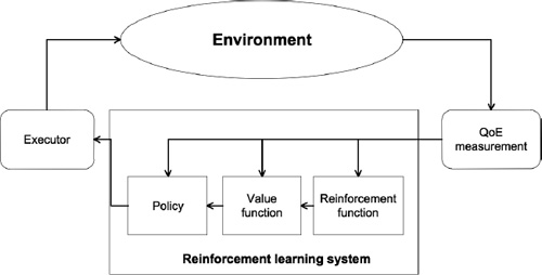
Definitively, the system integrates the QoE measurement in an evolutionary routing system in order to improve the user perception based on the Q-learning algorithm to choose the “best optimal QoE paths” (Figure 4.4). For our method, we have mapped the RL model onto our routing model in the context of a learning routing strategy. So in that way, the routing process is built in order to maintain the best user perception.

Figure 4.4. Q-learning-based model

As mentioned previously, integrating QoE into a system reduces the complexity problem associated with NP-completeness of the QoS model. The objective function is related to user satisfaction, that is the selection of certain parameters, or even one, not several, uncorrelated parameters. We work on the oriented selection gradient on this parameter. In this section, first, we present our formal parametric model based on a continuous time evolving function to prove the convergence of our approach. We then describe in detail the QQAR algorithm. The learning and selection processes explain the way we apply the Q-learning algorithm to QQAR.

4.6.1. Formal parametric model

Our system is based on different modules. Each module optimizes a local cost function. To achieve this, we propose a unified formal model to determine the convergence of our approach. Continuous learning in our system involves changing the parameters of the network model using an adaptive update rule as follows:

[4.25]

where w(n) denotes the parameters of the whole system at time n, x(n) is the current traffic and e is the modification step. F is either the gradient of a cost function or a heuristic rule. x can be defined by a probability density function p(x) and w is the parameters of the learning system. The concept behind our system is based on the fact that each iteration uses an instance of a real flow instead of a finite training set. The goal of this learning system consists of finding the minimum of a function C(w), called the expected risk function, and the average update is therefore a gradient algorithm which directly optimizes C(w). For a given state of the system, we can define a local cost function J(x, w) which measures how well our system behaves on x. The goal of learning is often the optimization of some function of the parameters and of the concept to learn which we will call the global cost function. It is usually the expectation of the local cost function over the space x of the concept to learn:

[4.26]

Most often we do not know the explicit form of p(x) and therefore C(w) is unknown. Our knowledge of the random process comes from a series of observations x_i of the variable x. We are thus only able to calculate J(x, w) from the observations x_i

A necessary condition of optimality for the parameters of the system is:

[4.27]

where Δ is the gradient operator. Since we do not know ΔC(w) but only the result of Δ_w J(x, w), we cannot use classical optimization techniques to reach the optimum. One solution is to use an adaptive algorithm as follows:

[4.28]

where γ is the gradient step. There is a close similarity between equations [4.25] and [4.28], and when learning in the second stage aims at minimizing a cost function, there is a complete match. This formulation is particularly adequate for describing adaptive algorithms that simultaneously process an observation and learn to perform better. Such adaptive algorithms are very useful in tracking a phenomenon that evolves over time, as in user perception.

4.6.2. QQAR algorithm

Our approach is based on the Q-learning algorithm. In this section, we summarize some general idea of RL and Q-learning.

Q-learning [WAT 92a] is a technique for solving specific problems by using the RL approach [SUT 98]. Even though the RL has been around for a long time, this concept has been applied/used recently in many works in many disciplines, such as game theory, simulation-based optimization, control theory and genetic algorithms. Here we cite here some recent RL advances: RL-Glue [TAN 09], PyBrain [SCH 10], Teachingbox [ERT 09], etc.

Here we explain how an RL framework works. In an RL framework, an agent can learn control policies based on experience and rewards. In fact, MDP is the underlying concept of RL.

An MDP model is represented by a tuple (S, A, P, R), where S is the set of states, A is the set of actions and P(s′|s, a) is the transition model that describes the probability of entering state s′ after executing action a at state s. R(s, a, s′) is the reward obtained when the agent executes a at state s and enters s′. The quality of action a at state s is evaluated by Q-value Q(s, a).

Solving an MDP is equivalent to finding an optimal policy π : S → A that maps states to actions such that the cumulative reward is maximized. In other words, we have to find the following Q-fixed points (Bellman equation):

[4.29]

where the first term on the right side represents the expected immediate reward of executing action a at s; the second term represents the maximum expected future reward and γ represents the discount factor.

One of the most important breakthroughs in RL is an off-policy temporal difference (TD) control algorithm known as Q-learning, which directly approximates the optimal action-value function (equation [4.29]), independent of the policy being followed. After executing action a, the agent receives an immediate reward r from the environment. By using this reward and the long-term reward it then updates the Q-values influencing future action selection. One-step Q-learning is defined as:

[4.30]

where α is the learning rate, which models the rate of updating Q-values.

In order to apply the Q-learning algorithm to our routing system, we have mapped the RL model onto our routing model in the context of learning a routing strategy. We consider each router in the system as a state. The states are arranged along the routing path from the client to the chosen server in a CDN. Furthermore, we consider each link emerging from a router as an action to choose. The system’s routing mechanism refers to the policy π (Table 4.1). Regarding QoE measurement, we used a method that evaluates the QoE of all nodes.

The routing mechanism is illustrated in Figure 4.5

Figure 4.5. QQAR protocol

Figure 4.6 describes the QQAR algorithm.

Figure 4.6. QQAR diagram

In the following two sections, we clarify the two main processes of QQAR: the learning process and the selection process.

4.6.3. Learning process

As the analysis of Q-learning algorithm presented previously, we present a new method for network exploration. This technique relies on forward exploration [BOY 94] to which we added a probabilistic mechanism exploration. This mechanism allows us, first, to explore from time to time optimal paths and, second, to avoid further congestion of the network as data packets are also used for exploration.

In our model, each router has a routing table that indicates the Q-values of links emerging from this router. For example, in Figure 4.7, node y has a routing table containing Q values: Q_yz1, Q_yZ2 , Q_yZ3 … Q_yZn corresponding to n links from y to z_i with i = 1,…, n. Based on this routing table, the optimal routing path can be trivially constructed by a sequence of table look-up operations. Thus, the task of learning optimal routing strategy is equivalent to finding the Q-fixed points (equation [4.29]).

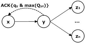
Figure 4.7 Learning Process

As mentioned above, after receiving a data packet, the destination node (end user) evaluates the QoE. Then, it sends back the feedback (QoE value) as ACK message to the routing path. Each router x in the routing path receives this message, including the QoE evaluation result (the MOS score²) of the previous router (q_y) and the maximum value of Q-values (max Q_yz) in the routing table of node y (Figure 4.7).

Based on the native Q-learning algorithm (equation [4.30]), the update function is expressed as:

[4.31]

where Q_new and Q_old are the new and old Q-values, respectively. The Q_{new estimation} is the new estimation of Q-values from nodes x to the destination, depending on the following two factors:

1) The estimation of the link xy, expressed by the difference between the Q-values of node x and y. We call that the immediate reward. The reason of choosing this estimation is explained below.

2) The optimal estimation from node y to the destination, expressed by the maximal value among the Q-values in the Q-table of node y. We call that the future reward.

So, we have the Q-value of the new estimation expressed in equation [4.32]:

[4.32]

where β and γ are two discount factors balancing the values between future reward and immediate reward.

From two equations [4.31] and [4.32], router x updates the Q-value of the link xy by using the update function defined in equation [4.33]:

[4.33]

where Q_xy and Q_yzi are Q-values of links xy and yz_i. q_x and q_y are QoE value evaluated (MOS score) by using the QoE measurement method at node x and y. α is the learning rate, which models the rate updating Q-value. Actually, it is worthwhile noting here the close similarity between equation [4.33] and [4.28] given in the global cost function. Parameters a and Q represent the gradient step γ and the function J in the formal model respectively (equation [4.28]). In fact, QQAR becomes reactive with the update function in equation [4.33]. The router will reduce the Q-value of a link when its quality is degraded. This reduction helps QQAR to actively avoid bad quality links.

Algorithm 4.2 Learning algorithm

Input: [Q₀, Q₁, Q₂, Q_m]: Q-values in Q-table.

m: The number of neighbor nodes.

N: the number of node of the routing path.

for i = 0 to N do

Receive the ACK message;

Update the Q-value;

Find the maximal Q-value and attach it to the ACK message;

Forward the ACK message;

end for

According to the time complexity of the learning algorithm (algorithm 4.2), the learning process is executed N times with N the number of node throughout the routing path. In addition, the number of operations for finding maximal Q-value in the Q-table is m, which is the number of neighbors of this node. As shown in algorithm 4.2, the number of elementary operations performed by the learning algorithm for a loop is (m + 3). In fact, there are totally N loops. So, the asymptotic time complexity of the learning algorithm is O(N × m).

4.6.4. Simple use case-based example of QQAR

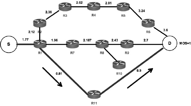
We now show some samples of execution of QQAR. We consider a simple network topology as shown in Figure 4.8. This network consist of 11 routers (R1, R2,..., R11), one source node, one destination node (the chosen server in a CDN) and 14 connection links. With this sample network, we have three paths from source to destination: R1-R2-R3-R4-R5-R6, R1-R7-R8-R9 and R1-R11. The path R1-R7-R8-R10 never reaches the destination. All routers used the QQAR algorithm. We fixed the three parameters α = β = γ = 0.9. In order to show the execution of the exploration phase easily, we have chosen this high value for these parameters to make the learning change rapidly. Note that the numbers appearing on the links in these figures are their Q-values.

Figure 4.8. Sample of execution for QQAR

In the first phase (Figure 4.9), assume that the path R1-R2-R3-R4-R5-R6 is chosen and the destination gives an MOS score of 4. We can see that after the update process, all the links of the routing path receive a high Q-value.

Figure 4.9. Phase 1: with MOS = 4, the Q-values are updated

In the second phase (Figure 4.10), the path R1-R7-R8-R9 is chosen. The destination has given an MOS score of 3.

Figure 4.10. Phase 2: with MOS = 3, the Q-values are updated

The path R1-R11 has been chosen in third phase (Figure 4.11). The destination has given a MOS score of 1. The Q-values in this routing path are updated by using equation [4.33]. This phase represents the case where a short routing path in terms of hop-count will have low QoE value if the end user is not satisfied with the received quality.

Figure 4.11. Phase 3: with MOS = 1, the Q-values are updated

In the fourth phase, the path R1-R7-R8-R10 is chosen (Figure 4.12). The packet cannot reach the destination, so the QoE value obtained is 0. We can see that our update function of equation [4.33] does not influence the Q-value in the paths R1-R7 and R7-R8. Therefore, the router R8 will never choose the path R8-R10 to forward the packet.

Figure 4.12. Phase 4: with MOS = 0, the Q-values are updated

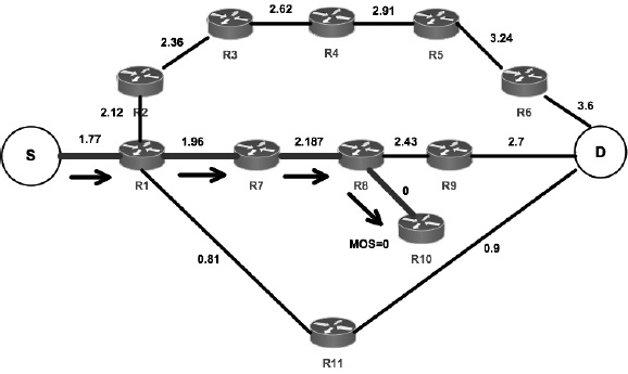
In the fifth phase, the path R1-R2-R3-R4-R5-R6 is chosen for the second time (Figure 4.13). We assume that the path quality is degraded compared with the first time. So, the MOS value given is just 2. The update process has decreased all Q-values of this path.

Figure 4.13. Phase 5: with MOS = 2, the Q-values are updated

The samples of algorithm execution above show some characteristics of exploration process of QQAR:

In order to explain why the new estimation in equations [4.32] and [4.33] depends on the difference of Q-values between two adjacent nodes, (q_y − q_x) we give another sample network in Figures 4.14 and 4.15. We keep the value of 0.9 for three parameters α, β and γ. This network includes nine routers, one destination and 16 connection links. The router R4 is connected to all other routers. We make router R4 connect to all other routers in order to analyze the Q-routing issue that is solved by our proposed difference in formulation [4.33].

In fact, due to the difference in the update function, the QQAR is able to detect exactly where the failure comes from. Figure 4.14 describes network state before the failure. With the MOS score of 3 obtained at the destination, all links have their own Q-values assigned by QQAR algorithm. When the failure occurs in the link R1-R4 (Figure 4.15) and the routing path is R1-R4-R7, the MOS score decreases from 3 to 1. The router R7 and R4 update the Q-values of links R7-D and R4-R7, which are equal to 1.08 and 1.11, respectively. We now analyze the update process of router R1. Without the difference of q_R4 and q_R1, the update function becomes:

Figure 4.14. Network before the failure

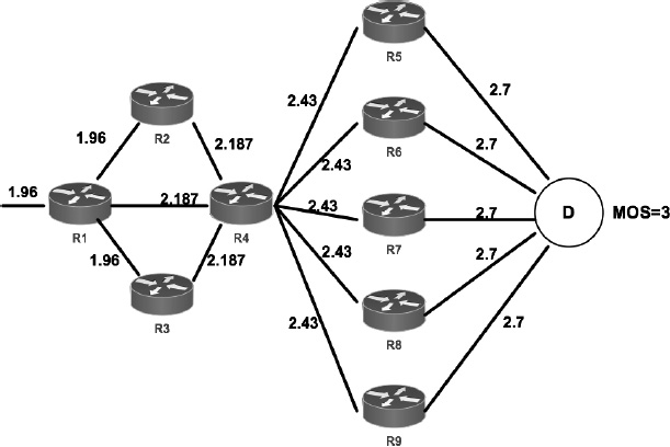
Figure 4.15. QQAR detects exactly the downed link

[4.34]

Since the highest value of Q-values of links emerging from R4, max_i Q_R4-Ri, is still 2.43, the Q-value of link R1-R4 is still 2.187. In reality, the problem of quality degradation comes from the link R1-R4. In order to solve this problem, we added the difference of Q-values between two adjacent routers (equation [4.33]). Adding this difference helps us to find the link that causes the quality degradation problem. In fact, this difference makes the Q-value of link R1-R4 decrease from 2.187 to 0.56 (Figure 4.15). With this new low Q-value, the future routing paths of QQAR will avoid this low-quality link.

In order to prove this advantage, we have tested two versions of the algorithm QQAR: QQAR-1 using formulation [4.33] as an update function and QQAR-2 using formulation [4.34] to update their Q-values. The only difference between them is the difference (q_y − q_x). We used the irregular network topology 6 × 6 grid (Figure 4.17). The test lasts 10 min. After 250 s, we make link R16-R25 break down to see how these two versions of QQAR react to this problem.

Figure 4.17. Irregular 6 × 6 grid network

As shown in Figure 4.16, after approximately 80 s of the initial period where two algorithms learn the network topology, they obtain an average MOS score of 4.0. At the 250th min, the MOS score obtained by two algorithms decreases to 1.5 since the link R16-R25 is broken down. Subsequently, while QQAR-2 takes 220 s to regain the MOS value of 4.5, the QQAR-1 takes just about 100 s. Therefore, in this example, the capacity of QQAR with the difference of Q-value between two adjacent nodes for reacting to the environment changes is better than the version without this difference.

Figure 4.16. Average MOS score of QQAR-1 and QQAR-2

So, with this efficient learning process, all nodes can use their updated Q-values in the Q-table to select the next node for routing the packet received. The selection process is presented in the following section.

4.6.5. Selection process

With regard to the selection process in each node after receiving a data packet, we have to consider the trade-off between exploration and exploitation. It cannot always exploit the link that has the maximum Q-value because each link must be tried many times to reliably estimate its expected reward. This trade-off is one of the challenges that arises in RL and not in other kinds of learning. To obtain good rewards, an RL agent (router) must prefer actions that it has tried in the past and found to be effective in producing reward. But to discover such actions, it tries actions that have not selected before. The agent has to exploit what it already knows, but it also has to explore in order to make better action selection in the future. There are some mathematical issues to balance exploration and exploitation. We need a method that varies the action probabilities as a graded function of estimated value. The greedy action (i.e. the action that gave the best quality feedback in the past) still has the highest selection probability. All the other actions are ranked and weighted according to their value estimates. Therefore, we have chosen the softmax method based on the Boltzmann distribution [SUT 98].

With these softmax action selection rules, after receiving a packet, node x chooses a neighbor y_k among its n neighbors y_i (i = 1,..., n) with probability expressed by equation [4.35] to forward the packet:

[4.35]

where Q_xyi is the Q-value of link xy_i and τ is the temperature parameter of Boltzmann distribution. High temperature makes the link selection be all equi-probable. On the contrary, low temperature generates a greater difference in selection probability for links that differ in their Q-values. In other words, the more we reduce the temperature τ, the more we exploit the system. Initially, we begin by exploring the system with the initial value of the temperature τ. Then, we increasingly exploit the system by decreasing this temperature value. In that way, we reduce τ after each forwarding time as shown in equation [4.36]:

[4.36]

where Ø is the weight parameter.

More precisely, the selection process can be summarized in algorithm 4.3:

Algorithm 4.3 Selection algorithm

Input: [Q₀, Q₁, Q₂, Q_n]: Q-values in Q-table.

repeat

  Receive the data packet;

  Look at the Q-table to determine the Q-value for each link;

  Calculate the probabilities with respect to Q-values (equation [4.35]);

  Select link with respect to the probabilities calculated;

  Decrease the temperature value (equation [4.36]);

until Packet reaches the destination

We now analyze the algorithm complexity of the selection algorithm (algorithm 4.3). There are N loops in total, where N is the number of node in the routing path. Calculating the probabilities for each link has a time complexity of O(m), where m is the number of neighbors. As , where is time to live we fixed before (i.e. the number of hops the packet is allowed to pass before it dies), the worst-case time complexity for the selection algorithm is .

4.7. Experimental results

In order to validate our studies, this section shows the experimental results of our two proposals: the routing algorithm QQAR and the new server selection method.

4.7.1. Simulation setup

We also implement a network simulation model to validate the proposals. First, we present the simulation setup including setting parameters, simulator and simulation scenario.

Table 4.2 lists the setting parameters.

Table 4.2. Simulation setup

4.7.1.1. Simulator

There are many network simulators (NSs) allowing the implementation and performance evaluation of network systems and protocols. They are either prototypes from academic research or marketed products. In this section, we present three common simulators: NS, MaRS and the optimized network engineering tool (OPNET). Subsequently, we present in detail the OPNET and explain why we have chosen these simulators to simulate our proposals.

4.7.1.1.1. NS

NS [NET 89] is distributed by the University of Berkeley (USA). This is a discrete event simulator designed for research in the field of networks. It provides substantial support for simulations using TCP and another routing protocols. The simulator is written in C++ and uses OTcl as the language interface and configuration control.

The advantage of NS is that it offers many extensions to improve its basic characteristics. The user specifies the network topology by placing the list of nodes and links in a topology file. Traffic generators can be attached to any node to describe its behavior (e.g. FTP or Telnet client). There are different ways to collect information generated during a simulation. Data can be displayed directly during the simulation or be saved to a file for processing and analyzing.

The two monitoring modes in NS are, first, the registration of each packet as it is transmitted, received and rejected and, second, the monitoring of specific parameters, such as the date of arrival of packets and size. Data generated during the simulation are stored in files and can be treated. The Network Animator is a tool for analyzing these files. Its graphical interface displays the configured topology and packet exchanges.

The NS is an open source simulator (its source code is available in [NET 89]). It is widely used for research in the field of networks, and recognized as a tool for experimenting with new ideas and new protocols.

4.7.1.1.2. MaRS

The Maryland routing simulator (MaRS) [MAR 91] is a discrete event simulator that provides a flexible platform for the evaluation and comparison of routing algorithms. It is implemented in language C under UNIX, with two GUIs: Xlib and Motif.

MaRS allows the user to define a network configuration consisting of a physical network, routing algorithms and traffic generators. The user can control the simulation, record the value of certain parameters and save, load and modify network configurations. MaRS consists of two parts: (1) a simulation engine, which controls the event list and the user interface; (2) a collection of components to model the network configuration and to manipulate certain features of the simulation. The configuration of the simulation (network algorithms, connections and traffic) can be done via configuration files or via a graphical X-Windows.

4.7.1.1.3. OPNET

The OPNET project was launched in 1987. Currently, this software is marketed by MIL3 and is the first commercial tool for simulation of communication networks.

This is a simulation tool based on discrete events, written in C. It has a graphical interface used in various modes, which facilitates the development of new models and simulation programs. Many models of protocols are provided with the standard distribution of OPNET, which is a definite advantage over other simulators. In fact, the other simulators often offer only an implementation of TCP/IP and some classical routing protocols. OPNET is a very flexible tool, which simulates a network at any level of granularity. It is used extensively in many development projects.

The advantages of this simulator tool motivate us to choose it in order to simulate and validate our proposals in this book. The following section presents, in detail, simulation settings using OPNET simulator.

4.7.1.2. Simulation scenarios

The Internet today has a dynamic environment with lots of unexpected changes that cause different network issues. The load balance is an important factor that influences the network performance. There are different load balancing methods that have been introduced to avoid this issue. In fact, overloaded routers or servers can break down the entire network system rapidly. In addition, unexpected incidents also affect the network service quality. A failed router or link can change the network topology. This change really decreases the network quality and requires an effective fault-tolerance mechanism of the network operator. Therefore, we simulate the following two scenarios:

Figure 4.18. Incident time line for router X

4.7.1.3. Simulation metrics

In this book, we used the following metrics to evaluate the performance of the approaches:

4.7.1.4. Dynamic network system

One of the most important capacities of a routing algorithm is adapting to changes in crucial system parameters during network operation. In addition, the Internet today always changes dynamically. Therefore, we tested our approaches on networks whose topology, end user requests distribution and traffic load levels were dynamically changing.

4.7.1.5. Simulation settings

For performance validation of the proposals, we have chosen the simulator OPNET for several reasons. It allows us to visualize the physical topology of a local, metropolitan, remote or embedded network. The protocol-specified language is based on the formal description using finite state automata. It is also easier to understand the problems of transit times and network topology.

OPNET has three nested hierarchical levels: the network domain, the domain node and the process domain. In the following sections, we present our simulation settings of these levels.

4.7.1.5.1. Network domain

This is the highest level of the hierarchy of OPNET. It defines the network topology by deploying hosts, links and active equipment such as switches or routers. Defined by its model, each communication entity (called node) is configurable. The graphical user interface associated with the network domain takes into account the spatial deployment of the network. According to the network, we worked on the three following topologies: 6 × 6 GridNet, 3AreasNet and NTT. We have chosen a testing methodology as follows.

– 6 × 6 GridNet (Figure 4.19b): First, we tested our routing algorithm on a simple network, the 6 × 6 GridNet, to verify its functionality. This irregular network was first used by Boyan and Littman [BOY 94]. Then, it was widely used and accepted in routing protocols studies. The network consists of two connected areas with a bottleneck of traffic on two bridging links. After obtaining sufficient results for the first topology, we continued testing our algorithm by using the second topology, the 3AreasNet.

Figure 4.19. Network topologies. For a color version of the figure, see www.iste.co.uk/mellouk/qoe

– 3AreasNet (Figure 4.19a): For the second testing step, we ourselves have designed a simulated irregular network, called 3AreasNet, with three separated areas including 35 routers. Each area is connected to each other by a unique link and all links are similar. This constitutes our second beta test bed, which is used to test the functionality of algorithms. The 3AreasNet topology is based on Waxman topology [WAX 93]. This method distributed the node uniformly in the network, and the edges are added considering the probability defined by equation [4.42] that depends on the distances between nodes.

[4.42]

where d represents the distance between two nodes, L is the maximum distance in the network, α > 0 and β < = 1. The parameter α increases or decreases the probability of edges between two nodes and β controls the ratio of long/short edges.

– NTT [DIC05]: For the third step, we worked on the NTT network that is modeled on the exact characteristics of a real-world network, the former Nippon Telephone and Telegraph (NTT) company fiber-optic corporate backbone. NTTnet is a 57 node, 162 bi-directional link network (Figure 4.19c). Unlike the 3AreasNet and 6 × 6 GridNet topologies that are used to test the functionality of algorithms, this topology is used to validate the proposed approaches.

In each network, we used 10 end users (red color), 10 iBoxes (yellow color) and five replica servers (green color). According to the server placement, we used a server placement method proposed in [QIU 01]. This method is based on a greedy algorithm [KRI 00]. For this method, we have to choose five servers in potential sites. The site having the lowest cost (hop-count to end users) is chosen. Then, the iteration continues until five servers have been chosen. According to the cache organization, we assume that all requested data is stored in each server.

4.7.1.5.2. Node domain

Node domain is used to define the formation of nodes (e.g. routers, workstations and hubs). The model is defined by using blocks called modules. Some modules are not programmable: it is primarily transmitters and receivers, whose unique function is to interface the node and links. On the other hand, other modules are programmable such as processors and queues.

Processors are modules that perform a specific task node. They symbolize the different parts of the operating system of a machine, and the different layers mainly implemented in the node network (e.g. Ethernet and IP). In addition, these modules can communicate with each other via packet streams, which allow a packet to transit from one layer to another within the same machine. This kind of organization provides a clear vision for the protocol stack implemented in a node, and quickly understands their interactions. For example, the IP module is connected to the layer 4 modules such as TCP, UDP, and those of layer 2 (Ethernet). The statistic wires are the second type of links for communication between modules. They can be traced back the statistics from one module to another, such as the size and the delay of queues of the transmitter.

Process domain defines the role of each programmable module. A module has a default main process, which can add sub-processes performing a sub-task. OPNET provides mechanisms for all processes created within a process domain to communicate with each other via a shared memory block or scheduling interrupts. The role of a module is determined by the process model, which is described as a finite state machine. Each block represents a different state, wherein the machine executes a specific code. Transitions refer to links between blocks and are determined by conditions (interruptions, variable with some value, etc.). Actions to perform are written in language C. OPNET provides a library of over 400 proprietary functions specific to the use of networks (creating, sending and receiving packets, extracting values in different fields of a header, etc.).

4.7.1.5.3. Network traffic model

In order to model the real-word Internet Traffic, we studied the performance of algorithms with increasing packet traffic load. According to the traffic model, we used MMPP [OKA 09] as arrival traffic process. First, this section presents briefly the traditional Poisson process. Then, we describe the MMPP and explain why we have chosen this traffic model.

– Traditional Poisson process:

In traditional traffic theory, the Poisson arrival process [KIN 93] was very suitable for data and voice transmission. It is a discrete probability distribution, which describes a random variable representing the number of events that occur in a time interval. In the Poisson arrivals model, there is a convenient relationship between Poisson (discrete) and Exponential (continuous) distributions. The Poisson distribution represents the number of events in a time interval. On the other hand, the exponential distribution represents time between events. The Poisson arrival model gives the following probability of k arrivals in a unit of time (1 s):

[4.43]

According to inter-arrival time, equation [4.44] expresses the exponential distribution of inter-arrival times:

[4.44]

The Poisson arrival process has some properties for analysis [CHE 07]:

– It is memoryless. If the previous arrival occurred T time ago, the time to the next arrival will be exponentially distributed with a mean of regardless of T.

– The number of arrivals in an interval of length t has a Poisson distribution with mean λt.

– The sum of two independent Poisson arrival processes is a Poisson process with a rate of the sum of these Poisson processes. For example, the sum of two Poisson processes with rates λ₁ and λ₂ is a Poisson process with rate λ₁ + λ₂.

– Markov-modulated Poisson process (MMPP):

Since the arrival rate λ of the Poisson process is constant, it is obviously unrealistic as a traffic model. For example, with the aggregation of multiple packet speech flows, the starting and terminating times are random times, so the flow rate is not constant. MMPP has been introduced to solve this issue. The MMPP method modulates the Poisson rate as the states of a continuous-time Markov chain. The MMPP has the memoryless property of the Poisson process and can be analyzed by Markov theory. The complexity of the analysis increases with the number of states, so this number is usually small.

Definitively, we have designed a Markov chain with three states of rate values: 1, 4 and 10 (Figure 4.20). In Figure 4.20, three states represent three rate values. The number on each transition arrow is the probability of state transition.

Figure 4.20. Poisson rate modulated by Markov chain

Applying MMPP method gives us the experiment results in Figure 4.21, which shows the switch between the states following the Markov chain in Figure 4.20. The axis y in these figures represents the number of arrival process in 1 s and the axis x is the time (in second). Taking an example of Figure 4.21a, it makes a switch from state of λ =1 to state of λ = 4 at the 300th s. Subsequently, at the 650th s, it returns to the state of λ =1. Then, during about 120 s from the 780th s to the 900th s, the state is λ =10. The switch between the states follows the Markov chain in Figure 4.20. The x-axis follows the exponential distribution given in equation [4.44] with the A being the value of current λ.

Figure 4.21. Markov-modulated Poisson process

In this book, we used the MMPP model to implement the arrival process for the user request model. Actually, using the MMPP model gives a traffic model with different load level for network system. In fact, the higher the value of λ is, the more the network system is loaded.

4.7.2. Experimental setup

To validate the results of QQAR, we compare our approach with three kinds of algorithm:

While we can use static routing for small networks like local area networks (LAN), larger (or huge) networks like the Internet have complex topologies that need adaptive routing protocols, which attempt to solve this problem by constructing routing tables automatically. Three adaptive routing algorithms described above are representative of today’s widely used routing systems. This motivates us to use them to compare with our proposed routing algorithm.

The comparison in our experiment is based on the average MOS score, PDR and NRO that represents the QoE value. For the video streaming, we used two types of video: the Standard Definition Video (SD Video) and the High-Definition Video (HD Video). The resolution of SD Video is 768 × 576, while the resolution of HD Video is 1,280 × 720 pixels (720p). We use the HD Video with large volume files to test networks with lots of loaded flows. In other words, we intend to test our network in different load levels. The first set of experiments was conducted by using the SD video files for video streaming. Then, we use the HD Video files to test our approach in a stressed network. Finally, we stressed the network by adding some data flow with different load levels.

We observe the average MOS score at 10 access points and the experiment has been relaunched 10 times as a cross-validation method. The average MOS value is calculated with sliding windows of 1 h. We also present the confidence interval of 95%. The duration time is 45 h.

4.7.3. Average MOS score

Figures 4.22, 4.23 and 4.24 illustrate the experimental result of average MOS scores of four algorithms in three network topologies: the 3AreasNet, the 6 × 6 GridNet and the NTTnet, respectively. As mentioned previously, for each topology, we implement two types of video: the SD Video and the HD Video. For these experiments, we collect the MOS score every 5 h.

In observing Figure 4.22a and 4.22b, we see that after the first 5 h, the four protocols obtain the stable MOS score. These stable values are 4.1, 3.3, 2.95 and 2.6 for QQAR, SOMR, SPF and DV, respectively (Table 4.3).

Figure 4.22. MOS score for 3AreasNet topology

Table 4.3. MOS score for SD Video streaming of 3AreasNet topology

According to the effect of network load on the results, video streaming with HD Video depresses QoE value of four protocols with the decrease from 4.1 down to 3.65, 3.3 to 3.2, 2.95 to 2.8 and 2.6 to 2.45 for QQAR, SOMR, SPF and DV, respectively (Table 4.4).

Table 4.4. MOS score for HD Video streaming of 3AreasNet topology

Even the HD Video streaming decreases the QoE value of protocols, the obtained MOS score of QQAR is better than the three other ones with the improvement of 148.97%, 114.06% and 130.35% for DV, SOMR and SPF, respectively.

Table 4.5. MOS score for SD Video streaming of 6 x 6GridNet topology

Similarly, in the 6 × 6GridNet topology (Figure 4.23), the four protocols obtain the stable MOS scores: 4.1, 3.2, 3.5 and 3.35 for QQAR, DV, SOMR and SPF, respectively. The HD Video streaming lowers the MOS scores for several approaches: 4.1 down to 3.9, 3.2 to 3.15, 3.35 to 3.3 for QQAR, DV and SPF, respectively. This decrease of MOS score is negligible. The SOMR is not affected by the increase of load.

Figure 4.23. MOS score for 6 x 6GridNet topology

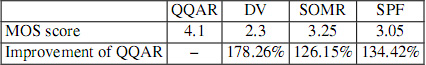
We now analyze the results by using NTTnet topology (Figure 4.24). According to the SD Video streaming, the average MOS scores of QQAR, SOMR, SPF and DV are 4.1, 3.25, 3.05 and 2.3, respectively (Table 4.7). For the HD Video streaming, the QQAR, SOMR, SPF and DV obtain, respectively, MOS scores of 3.9, 2.9,2.8 and 2.3.

Figure 4.24. MOS score for NTTnet topology

Table 4.6. MOS score for HD Video streaming of 6 x 6GridNet topology

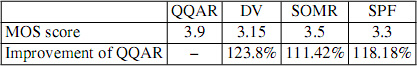
Table 4.7. MOS score for SD Video streaming of NTT topology

Table 4.8. MOS score for HD Video streaming of NTT topology

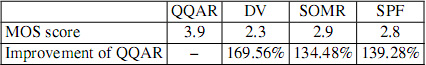
We have the same conclusion as the previous topology: the obtained MOS score of QQAR is better than the three others in both types of video streaming.

In three networks: 3AreasNet, 6 x 6GridNet and NTTnet (Figures 4.22, 4.23 and 4.24), the algorithm QQAR gives better QoE value than the three others. That is explained by the following reasons:

According to the DV algorithm, it is the most widely accepted routing protocol. It is straightforward in broadcasting their entire current routing database periodically, typically every 30 s. The name “distance-vector” means that there is a distance (a cost) and a vector (a direction) for each destination. The DV algorithm works well for small, stable networks. This explains that it obtains a better QoE result in 3AreasNet and 6 × 6grid topology than NTTnet topology. In addition, there are some drawbacks of DV algorithms:

These arguments explain the worst QoE results of DV compared with the three other ones.

For SPF algorithm, it is considered as a link-state algorithm. The SPF is better suited than DV for large and dynamic networks. This explains the fact that SPF obtain better results than the DV algorithm. However, in a large network, a link change can lead to a flood of thousands of link-state messages that propagate across the entire network. In each router, the database storing these messages can be quickly overloaded. Each time there is a network change, routers must redetermine new paths. Fortunately, SPF is designed to resolve this issue by devising the SPF area. SPF areas are subdivisions of an entire network. More precisely, in the 3AreasNet topology (Figure 4.19a), SPF configures by dividing the network into three separated areas. In the 6 × 6GridNet topology (Figure 4.19b), the network is divided into two separated parts. SPF routers in one area do no exchange topology updates with the routers in the other areas. This reduces the update message(s) number of flows through the network. This improvement is shown clearly in our convergence time studies.

According to the SOMR algorithm, it is useful for finding multiple paths between a source and a destination in a single discovery. This multiple paths-based algorithm can be used to react to the dynamic and unpredictable topology change in networks. For example, when the shortest path found in using Dijkstra’s algorithm is not available for some reason, it is necessary to find the second shortest path. These paths are considered as k-shortest paths. This advantage explains the good MOS scores of the previous experiments: 3.3–3.2 in 3AreasNet, 3.5 in 6 × 6GridNet and 3.25–2.9 in NTTnet. The only drawback of this kind of algorithm is the time taken to calculate the k-shortest path. This algorithm is used several times to calculate the k-shortest path with k > 1. Because of this computational complexity, the SOMR obtains a lower quality than QQAR. In addition, the considered cost of SOMR is a linear combination of network parameters. However, the QoE depends not only on technical criteria but also on the human perception, which is an important subjective factor that we have considered in our proposals. More precisely, in our QoE measurement method, we determine the QoE by using a hybrid way that combines objective and subjective methods.

4.7.4. Convergence time

We now discuss the convergence time of these approaches. Network convergence is a notion that is used under various interpretations. In a routing system, every participating router will attempt to exchange information about the network topology. Network convergence is defined as the process of synchronizing network forwarding tables from the beginning (the initialization phase) or after a topology change. When there are no more forwarding tables changing for “some reasonable” amount of time, the network is said “converged”. For the learning routing algorithms like QQAR, the convergence time refers to the initialization phase for exploring the network environment. After this phase, such an algorithm becomes stable.

The three Figures 4.25, 4.26 and 4.27 show the obtained MOS scores of four algorithms in the first 5 min of simulation. The MOS scores are taken every 10 s. We consider three cases: for 3AreasNet (Figure 4.25), 6 × 6GridNet (Figure 4.26) and NTTnet (Figure 4.27) topologies. The goal is to study the convergence time of each approach in the initialization phase. All of the four algorithms have a common feature: in the initialization period, they have no information about the system. So, during this period, they try to explore the network. We call this period the initialization phase.

Figure 4.25. Initialization phase for 3AreasNet topology

Figure 4.26. Initialization phase for 6 x 6GridNet topology

Figure 4.27. Initialization phase for NTTnet topology

As shown in Figure 4.26, in the 6 × 6GridNet topology, the convergence times are 20, 90, 110 and 130 s, respectively, for SPF, QQAR, SOMR and DV. For the 3AreasNet network, the convergence times are 20, 90, 110 and 130 s for SPF, QQAR, SOMR and DV, respectively. For the NTTnet, the convergence times are 20, 110, 120 and 150 s for SPF, QQAR, SOMR and DV, respectively (Table 4.9). The larger the network is, the more time it takes for convergence.

Table 4.9. Convergence time

According to the DV algorithm, it is considered as a slow convergence routing algorithm due to the slow propagation of update messages. The DV routers periodically broadcast their routing database every 30 s. Especially, in large or slow link networks, some routers may still publicize a disappeared route. This explains the long convergence time of the DV algorithm shown in Table 4.9. It obtains the stable QoE value after 130 s in 3AreasNet and 6 × 6GridNet network and 150 s in NTTnet network. DV convergence is the slowest one among the four algorithms.

In contrast to the DV, SPF algorithm converges quickly and accurately. In both network topologies, the small one (3AreasNet and 6 × 6GridNet) and the large one (NTTnet), SPF works very well with the obtained result shown in Table 4.9. It archives an impressive result of 20 s of convergence. As explained above, the SPF algorithm divides 3AreasNet into three separate areas and 6 × 6GridNet into two areas. The routers within one area do not exchange topology updates with the ones in the other areas, which reduces the number of update messages to alleviate the network load. So, these advantages make SPF the fastest algorithm in terms of convergence time among the four algorithms.

For the QQAR algorithm, the routers do not have knowledge of entire network. Each QQAR router has a routing table containing Q-values of their neighbors. The exchange phase between each router and their neighbors takes time for the convergence phase, especially in a large network like NTTnet. This explains the obtained results in Table 4.9: 80 and 90 s in 6 × 6GridNet and 3AreasNet, but 110 s in NTTnet. In fact, 110 s is still an acceptable duration for convergence time of a routing protocol.

The SOMR-based routing uses the diffusing update algorithm (DUAL) [GAR 93] to obtain loop-freedom at every instant throughout a route computation, while the DV algorithm meets temporary micro-loops during the time of re-convergence in the topology due to inconsistency of forwarding tables of different routers. Therefore, as shown in Table 4.9, SOMR gives better convergence time results than the DV algorithm. More precisely, these are 100, 110 and 120 s in 6 × 6GridNet, 3AreasNet and NTTnet, respectively.

4.7.5. Capacity of convergence and fault tolerance

We have also tested the algorithm’s capacity of convergence as well as fault tolerance when a change of topology occurred in the network. To implement this situation, we broke down the link R18-R19 of the 6 × 6GridNet topology (Figure 4.28) at the 20th h. After this change of topology, the two areas (the left and the right) of the 6 × 6GridNet network are connected by only one link: R16-R25.

Figure 4.28. 6 x 6 GridNet topology after breaking down the R18-R19 link

As shown in Figure 4.29, after the 7200th s where the link R18-R19 was broken, the MOS scores of the four algorithms decreased to a value of 1.7. According to the convergence time (Table 4.10), the three algorithms QQAR, SOMR and SPF take the same time as the convergence time for initialization phase (Figure 4.26). However, even after the convergence phase, the re-obtained MOS scores of these algorithms are lower than the ones before the topology change. More precisely, the QoE value decreases from 4 to 3.7 for QQAR, 3.6 and 3.4 for SOMR, 3-2.8 for SPF and 2.55 to 2.4 for DV. This fact can be explained as follows. After the topology change, the data exchange between two areas of 6 × 6GridNet network is realized only on one link: the link R16-R25. Therefore, the congestion issue of this link caused the quality degradation. One more notable comment, the DV algorithm has no convergence phase in this context because even before the topology change, it used just the link R16-R25 to exchange data between two areas. So, the disappearance of the link R18-R19 does not have much influence on the DV algorithm result.

Figure 4.29. MOS score after topology change

Table 4.10. Convergence time for a topology change

Figure 4.30 shows us the average of these four algorithms in different load levels formulated in [4.37]: from 10% to 70%. We can see that the more the system is loaded, the more the average MOS score decreases. However, at any load level, the average MOS score of QQAR is higher than the three other algorithms. For a load level of 10%, the MOS score of QQAR is 4.1 (note that 4 represents a good quality in MOS score range). Regarding the three other protocols, the maximum value obtained by SOMR is just 3.3 with a load level of 10%.

QQAR shows a better end-to-end QoE result than the three other algorithms in any load level and in the same network context. So, with our approach, despite network environment changes, we can maintain a better QoE than traditional algorithms. Thus, QQAR is able to adapt its decisions rapidly in response to changes in network dynamics.

Figure 4.30. User perception in different load levels

4.7.6. Control overheads

Our experimental works also consist of analyzing overheads of these protocols. The type of overhead we observe is the control overhead that is determined by the proportion of control packet number as compared to the total number of packets emitted. To monitor the overhead value, we have varied the node number by adding routers to the network system. So the observed node numbers are 38, 50, 60, 70, 80. The obtained results are shown in Figure 4.31.

We can see this the control overhead of our approach is constant (50%). This is explained by the equal number of control packets and data packets in QQAR. Each generated data packet leads to an acknowledgment packet generated by the destination node. The control packet rates of DV, SPF and SOMR are respectively 0.03, 0.4 and 0.1 (packet/s). This order explains the control overhead order in Figure 4.31. While the SPF algorithm has the highest value because of the highest control packet rate (0.4 packet/s) with multiple types of packets such as Hello packet, Link State (LS) Acknowledgment packet, LS Update packet and LS State request packet, the DV algorithm has the smallest overhead value with a control packet rate value of 0.03. We can also see that the higher the number of nodes, the higher the overhead. So, with a stable overhead, our approach is more scalable than these other three.

Figure 4.31. Control overhead

4.7.7. Packet delivery ratio

According to the packet delivery issue, Figure 4.32 shows the PDR of the algorithms. PDR is the ratio of the number of packets received by the destination (client nodes) to the total number of sent packets at server nodes. This is calculated by using equation [4.40]. Generally, the more the network is loaded, the more PDR decreases. The QQAR gives a good result in keeping the ratio at 100% until the network load level of 30%. The minimal value obtained is 87% at 70% of load level. The PDR of the three other algorithms decreases with the increase of network load level. When network load level reaches 70%, the PDRs are 87%, 70%, 61% and 49% for QQAR, SOMR, SPF and DV, respectively. So, the QQAR obtains the best result in terms of delivery ratio.

Figure 4.32. Packet delivery ratio

4.8. Conclusion

In this chapter, we present an example of routing systems based on the QoE notion. We have integrated the QoE measurement into the routing paradigm for an adaptive and evolutionary system, called QQAR. Definitively, the latter is based on Q-learning, an algorithm of RL, and used QoE feedback as a reward in the learning model. The goal is to guarantee end-to-end QoE of a routing system. A simulation conducted on a large, real test bed demonstrates that this kind of approach yields significant QoE evaluation improvements over other traditional approaches. More precisely, the simulation results showed that the QQAR algorithm performs better than the other approaches in terms of the following: (1) MOS for different network loads; (2) convergence time in initialization phase; and (3) control overhead.

1 In this book, we are working on optimizing the obtained QoE value, so for us the optimized value is the maximal value. Probably, in other approaches where we work on delay optimization, the optimized value is the minimal value.

2 Mean opinion score (MOS) gives a numerical indication of the perceived quality of the media received after being transmitted. The MOS is expressed in numbers, from 1 to 5, 1 being the worst and 5 the best. The MOS is generated by averaging the results of a set of standard, subjective tests where a number of users rate the service quality.