To predict a client subscription assessment, we use the deep learning classifier implementation from H2O. First, we set up and create a Spark session:

val spark = SparkSession.builder
        .master("local[*]")
        .config("spark.sql.warehouse.dir", "E:/Exp/") // change accordingly
        .appName(s"OneVsRestExample")
        .getOrCreate()

Then we load the dataset as a data frame:

spark.sqlContext.setConf("spark.sql.caseSensitive", "false");
val trainDF = spark.read.option("inferSchema","true")
            .format("com.databricks.spark.csv")
            .option("delimiter", ";")
            .option("header", "true")
            .load("data/bank-additional-full.csv")

Although there are categorical features in this dataset, there is no need to use a StringIndexer since the categorical features have small domains. By indexing them, an order relationship that does not exist is introduced. Thus, a better solution is to use One Hot Encodng, and it turns out that H2O, by default, uses this encoding strategy for enumerations.

In the dataset description, I have already stated that the duration feature is only available after the label is known. So it can't be used for prediction. Therefore, we should drop it as unavailable before calling the client:

val withoutDuration = trainDF.drop("duration")

So far, we have used Sparks built-in methods for loading the dataset and dropping unwanted features, but now we need to set up h2o and import its implicits:

implicit val h2oContext = H2OContext.getOrCreate(spark.sparkContext)
import h2oContext.implicits._implicit 

val sqlContext = SparkSession.builder().getOrCreate().sqlContext
import sqlContext.implicits._

We then shuffle the training dataset and transform it into an H2O frame:

val H2ODF: H2OFrame = withoutDuration.orderBy(rand())

String features are then converted into categorical (type "2 Byte" stands for the String type of H2O):

H2ODF.types.zipWithIndex.foreach(c=> if(c._1.toInt== 2) toCategorical(H2ODF,c._2))

In the preceding line of code, toCategorical() is a user-defined function used to transform a string feature into a categorical feature. Here's the signature of the method:

def toCategorical(f: Frame, i: Int): Unit = {f.replace(i,f.vec(i).toCategoricalVec)f.update()}

Now it's time to split the dataset into 60% training, 20% validation, and 20% test datasets:

val sf = new FrameSplitter(H2ODF, Array(0.6, 0.2), 
                            Array("train.hex", "valid.hex", "test.hex")
                            .map(Key.make[Frame](_)), null)

water.H2O.submitTask(sf)
val splits = sf.getResultval (train, valid, test) = (splits(0), splits(1), splits(2))

Then we train the deep learning model using the training set and validate the training using the validation set, as follows:

val dlModel = buildDLModel(train, valid)

In the preceding line, buildDLModel() is a user-defined function that sets up a deep learning model and trains it using the train and validation data frames:

def buildDLModel(train: Frame, valid: Frame,epochs: Int = 10, 
                l1: Double = 0.001,l2: Double = 0.0,
                hidden: Array[Int] = Array[Int](256, 256, 256)
               )(implicit h2oContext: H2OContext): 
     DeepLearningModel = {import h2oContext.implicits._
                // Build a model
    val dlParams = new DeepLearningParameters()
        dlParams._train = traindlParams._valid = valid
        dlParams._response_column = "y"
        dlParams._epochs = epochsdlParams._l1 = l2
        dlParams._hidden = hidden

    val dl = new DeepLearning(dlParams, water.Key.make("dlModel.hex"))
    dl.trainModel.get
    }

In this code, we have instantiated a deep learning (that is, MLP) network of three hidden layers, L1 regularization and that intended to iterate the training for only 10 times. Note that these are hyperparameters and nothing is tuned. So feel free to change this and see the performance to get a set of the most optimized parameters. Once the training phase is completed, we print the training metrics (that is, AUC):

val auc = dlModel.auc()println("Train AUC: "+auc)
println("Train classification error" + dlModel.classification_error())
>>>
Train AUC: 0.8071186909427446
Train classification error: 0.13293674881631662

About 81% accuracy does not seem good. We now evaluate the model on the test set. We predict the labels of the testing dataset:

val result = dlModel.score(test)('predict)

Then we add the original labels to the result:

result.add("actual",test.vec("y"))

Transform the result into a Spark DataFrame and print the confusion matrix:

val predict_actualDF = h2oContext.asDataFrame(result)predict_actualDF.groupBy("actual","predict").count.show
>>>

Now, the preceding confusion matrix can be represented by the following plot using Vegas:

Vegas().withDataFrame(predict_actualDF)
    .mark(Bar)
     .encodeY(field="*", dataType=Quantitative, AggOps.Count, axis=Axis(title="",format=".2f"),hideAxis=true)
    .encodeX("actual", Ord)
    .encodeColor("predict", Nominal, scale=Scale(rangeNominals=List("#FF2800", "#1C39BB")))
    .configMark(stacked=StackOffset.Normalize)
    .show()
>>>

Now let's see the overall performance summary on the test set—that is, test AUC:

val trainMetrics = ModelMetricsSupport.modelMetrics[ModelMetricsBinomial](dlModel, test)println(trainMetrics)
>>>

So the test accuracy in terms of AUC is 76%, which is not that great. But why don't we iterate the training an additional number of times (say, 1,000 times)? Well, I leave it up to you. But still, we can visually inspect the precision-recall curve to see how the evaluation phase went:

val auc = trainMetrics._auc//tp,fp,tn,fn
val metrics = auc._tps.zip(auc._fps).zipWithIndex.map(x => x match { 
    case ((a, b), c) => (a, b, c) })

val fullmetrics = metrics.map(_ match { 
    case (a, b, c) => (a, b, auc.tn(c), auc.fn(c)) })

val precisions = fullmetrics.map(_ match {
     case (tp, fp, tn, fn) => tp / (tp + fp) })

val recalls = fullmetrics.map(_ match { 
    case (tp, fp, tn, fn) => tp / (tp + fn) })

val rows = for (i <- 0 until recalls.length) 
    yield r(precisions(i), recalls(i))

val precision_recall = rows.toDF()

//precision vs recall
Vegas("ROC", width = 800, height = 600)
    .withDataFrame(precision_recall).mark(Line)
    .encodeX("re-call", Quantitative)
    .encodeY("precision", Quantitative)
    .show()
>>>

We then compute and draw the sensitivity specificity curve:

val sensitivity = fullmetrics.map(_ match { 
    case (tp, fp, tn, fn) => tp / (tp + fn) })

val specificity = fullmetrics.map(_ match {
    case (tp, fp, tn, fn) => tn / (tn + fp) })
val rows2 = for (i <- 0 until specificity.length) 
    yield r2(sensitivity(i), specificity(i))
val sensitivity_specificity = rows2.toDF

Vegas("sensitivity_specificity", width = 800, height = 600)
    .withDataFrame(sensitivity_specificity).mark(Line)
    .encodeX("specificity", Quantitative)
    .encodeY("sensitivity", Quantitative).show()
>>>

Now the sensitivity specificity curve tells us the relationship between correctly predicted classes from both labels. For example, if we have 100% correctly predicted fraud cases, there will be no correctly classified non-fraud cases and vice versa. Finally, it would be great to take a closer look at this a little differently, by manually going through different prediction thresholds and calculating how many cases were correctly classified in the two classes.

More specifically, we can visually inspect true positives, false positives, true negatives, and false negatives over different prediction thresholds, say 0.0 to 1.0:

val withTh = auc._tps.zip(auc._fps).zipWithIndex.map(x => x match {
    case ((a, b), c) => (a, b, auc.tn(c), auc.fn(c), auc._ths(c)) })

val rows3 = for (i <- 0 until withTh.length) 
    yield r3(withTh(i)._1, withTh(i)._2, withTh(i)._3, withTh(i)._4, withTh(i)._5)

First, let's draw the true positive one:

Vegas("tp", width = 800, height = 600).withDataFrame(rows3.toDF)
    .mark(Line).encodeX("th", Quantitative)
    .encodeY("tp", Quantitative)
    .show
>>>

Secondly, let's draw the false positive one:

Vegas("fp", width = 800, height = 600)
    .withDataFrame(rows3.toDF).mark(Line)
    .encodeX("th", Quantitative)
    .encodeY("fp", Quantitative)
    .show
>>>

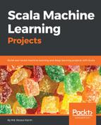
Then, it's the turn of the true negative ones:

Vegas("tn", width = 800, height = 600)
    .withDataFrame(rows3.toDF).mark(Line)
    .encodeX("th", Quantitative)
    .encodeY("tn", Quantitative)
    .show
>>>

Finally, let's draw the false negative ones as follows:

Vegas("fn", width = 800, height = 600)
    .withDataFrame(rows3.toDF).mark(Line)
    .encodeX("th", Quantitative)
    .encodeY("fn", Quantitative)
    .show
>>>

Therefore, the preceding plots tell us that we can increase the number of correctly classified non-fraud cases without losing correctly classified fraud cases when we increase the prediction threshold from the default 0.5 to 0.6.

Apart from these two auxiliary methods, I have defined three Scala case classes for computing precision, recall, sensitivity, specificity, true positives (tp), true negatives (tn), false positives (fp), false negatives (fn), and so on. The signature is as follows:

case class r(precision: Double, recall: Double)
case class r2(sensitivity: Double, specificity: Double)
case class r3(tp: Double, fp: Double, tn: Double, fn: Double, th: Double)

Finally, stop the Spark session and H2O context. The stop() method invocation will shut down the H2O context and Spark cluster respectively:

h2oContext.stop(stopSparkContext = true)
spark.stop()

The first one especially is more important; otherwise, it sometimes does not stop the H2O flow but still holds the computing resources.