10.4. Modeling Software Contention
The previous sections illustrated the effects of software contention on response time. This section briefly describes three approaches that can be used to build performance models that reflect the effect of software contention. The first two approaches are analytic and the last is based on discrete event simulation.
10.4.1. Simultaneous Resource Possession
The type of queuing networks (QNs) described in Section 9.4, can be solved exactly under a certain set of conditions. When these conditions hold, the QNs are said to have a product-form solution [3] [9] [11]. Product-form QNs do not allow a request to simultaneously hold more than one resource. This situation, called simultaneous resource possession, can be modeled only through approximate analytic models based on QNs.
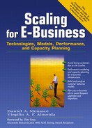
Software contention can be modeled through simultaneous resource possession as illustrated in Fig. 10.7. In this case, both software and hardware resources are part of the QN. The solid bars in Fig. 10.7 illustrate periods when a resource is being held by a request and the hashed bars indicate time spent waiting to seize a resource. The figure shows five time axes for the following resources: Web server thread, application server thread, database server thread, CPU at the database server, and I/O at the database server. The first three resources are software resources and the last two are hardware resources. A request arrives at time 1 at the Web server and queues for service by a Web server thread. Then, the request receives some processing at the Web server, which uses the CPU and I/O devices at the Web server machine. These two resources are used while simultaneously holding the Web server thread resource. Then, at time 3, the request joins the queue for service by an application server thread. While holding the application server thread, the request alternates holding the CPU and I/O resources at the application server machine (not shown in the picture). Then, at time 4, the request joins the queue for a database server thread. At this point, the request is already holding the Web server and application server threads simultaneously. When the request obtains a database server thread, at time 5, it alternates between waiting and using the CPU and I/O resources as shown in the figure. For example, when the request is using the CPU at the database server machine, it is simultaneously holding the following resources: a Web server thread, an application server thread, a database server thread, and the CPU at the database server machine. In other words, the request is holding the three software resources and one hardware resource at the same time.
Figure 10.7. Simultaneous Resource Possession of Software and Hardware Resources.

Various approximations have been proposed to deal with the issue of simultaneous resource possession in QNs and software delays [1] [6] [8] [10] [16].
10.4.2. Method of Layers
Due to its multi-tier architecture, e-business sites are suitable for representation by models composed of multiple layers. An extension to QNs, called Layered Queuing Networks (LQNs), is quite suitable for representing the software and hardware hierarchy in an e-business site [13] [17]. LQNs are queuing network models that combine contention for both software and hardware components, such as processors, disks, and networks.
In a LQN model, processes with similar behavior form a group or a class of processes. These processes may invoke services from lower level processes, which may represent software and/or hardware resources. For example, Fig. 10.8 shows a layered queuing model of an e-business site. We assume in the figure that the Web server is running on a machine of its own and that the application and database servers share another machine. However, the application server uses disk 2 and the database server uses disks 3 and 4. Web server threads are at level 1 of the LQN model and request services from CPU 1, disk 1, and application server threads, which are at level 2 of the LQN. The application server threads use disk 2 and the database server threads at level 3. Finally, the database server threads use CPU 2 and disks 3 and 4, which are at level 4.
Figure 10.8. Layered Queueing Network (LQN) Model.

Approximate analytic techniques based on Mean Value Analysis (MVA) are used to estimate performance measures of layered queuing models with L levels. Two of these techniques are the Method of Layers [13] (MOL) and Stochastic Rendez-vous Networks (SRNs) [17]. The MOL is an iterative technique that decomposes an LQN into a sequence of two-level QN submodels that are solved using MVA-based solution techniques. Performance estimates for the QN at each submodel are calculated and used as input for subsequent QN models. The goal of the MOL is to obtain a fixed point where mean performance measures (i.e., response time, utilization, and queue length) are consistent across all levels. The MOL solution method consists of an iterative algorithm that begins by assuming no hardware or software contention. The algorithm iterates until the response times of successive groups reach a fixed point [13]. A tool that implements these techniques is described in a paper by Franks et al [5].
Although SRNs are similar to MOLs in modeling capability, its solution technique differs from the approach used by the MOL. A SRN generalizes the client/server relationship to multiple layers of servers with send-and-wait interactions (rendez-vous). In a SRN, tasks represent software and hardware resources that may execute concurrently. Random execution times and communication patterns are associated with the tasks of a SRN [17].
10.4.3. Simulation
Simulation is the modeling technique of choice when obtaining exact or adequately accurate analytic models is very difficult for the system to be modeled. Simulation models mimic the behavior of a real system through computer programs that randomly generate events such as arrivals of requests and move these requests around through the various simulated queues. Several counts accumulate metrics of interest such as total waiting time in a queue and total time a resource was busy. These counts can be used at the end of the simulation to obtain average waiting times, average response times, and utilization of the various resources [7].
Simulation programs can be written in general purpose programming languages (e.g., C or C++), in general purpose programming languages augmented by simulation libraries (e.g., CSIM 18 [12] or SimPack [4]), in special purpose simulation languages (e.g., GPSS/H [2] or Simscript II.5 [15]), or in graphical languages supported by simulation packages that offer a GUI through which resources and flow of requests are described (e.g., SES/workbench [14]). To provide readers with an example of simulation programs, GPSS/H programs that model the situations depicted in the examples of the previous section are available at the book's website (see the Chapter 10 link).
Simulation is usually much more computationally intensive than analytic models. On the other hand, simulation models can be made as accurate as desired. However, more detailed simulation models tend to require more detailed data and more time for execution, thus increasing the cost of using simulation. Analytic models, even approximate ones, are, in general, the technique of choice for scalability analysis and for capacity planning.