Chapter 3. Some fundamentals

This chapter covers

• Scala philosophy, functional programming, and basics like class declarations
• Spark RDDs and common RDD operations, serialization, and Hello World with sbt
• Graph terminology

Using GraphX requires some basic knowledge of Spark, Scala, and graphs. This chapter covers the basics of all three—enough to get you through this book in case you’re not up to speed on one or more of them.

Scala is a complex language, and this book ostensibly requires no Scala knowledge (though it would be helpful). The bare basics of Scala are covered in the first section of this chapter, and Scala tips are sprinkled throughout the remainder of the book to help beginning and intermediate Scala programmers.

The second section of this chapter is a tiny crash course on Spark—for a more thorough treatment, see Spark In Action (Manning, 2016). The functional programming philosophy of Scala is carried over into Spark, but beyond that, Spark is not nearly as tricky as Scala, and there are fewer Spark tips in the rest of the book than Scala tips.

Finally, regarding graphs, in this book we don’t delve into pure “graph theory” involving mathematical proofs—for example, about vertices and edges. We do, however, frequently refer to structural properties of graphs, and for that reason some helpful terminology is defined in this chapter.

3.1. Scala, the native language of Spark

The vast majority of Spark, including GraphX, is written in Scala—pretty much everything inside Spark is implemented in Scala except for the APIs to support languages other than Scala. Because of this Scala flavor under the hood, everything in this book is in Scala, except for section 10.2 on non-Scala languages. This section is a crash course on Scala. It covers enough to get you started and, combined with the Scala tips sprinkled throughout the book, will be enough for you to use Spark. Scala is a rich, deep language that takes years to fully learn.

We also look at functional programming because some of its ideas have had a strong influence on the design of Spark and the way it works. Although much of the syntax of Scala will be intelligible to Java or C++ programmers, certain constructs, such as inferred typing and anonymous functions, are used frequently in Spark programming and need to be understood. We cover all the essential constructs and concepts necessary to work with GraphX.

Its complexity is not without controversy. Although Scala affords power, expressiveness, and conciseness, that same power can sometimes be abused to create obfuscated code. Some companies that have attempted to adopt Scala have tried to establish coding standards to limit such potential abuses and emphasize more explicit and verbose code and more conventional (purists would say less functional) programming styles, only to find that incorporating third-party Scala libraries forces them to use the full gamut of Scala syntax anyway, or that their own team of Java programmers weren’t able to become fully productive in Scala. But for small high-performance teams or the solo programmer, Scala’s conciseness can enable a high degree of productivity.

3.1.1. Scala’s philosophy: conciseness and expressiveness

Scala is a philosophy unto itself. You may have heard that Scala is an object-functional programming language, meaning it blends the functional programming of languages like Lisp, Scheme, and Haskell with the object-oriented programming of languages like C++ and Java. And that’s true. But the Scala philosophy embodies so much more. The two overriding maxims of the designers and users of Scala are as follows:

1.  Conciseness. Some say that it takes five lines of Java code to accomplish the same thing as one line of Scala.

2.  Expressiveness sufficient to allow things that look like language keywords and operators to be added via libraries rather than through modifying the Scala compiler itself. Going by the name Domain Specific Languages (DSL), examples include Akka and ScalaStorm. Even on a smaller scale, the Scala Standard Library defines functions that look like part of the language, such as &() for Set intersection (which is usually combined with Scala’s infix notation to look like A = B & C, hiding the fact that it’s just a function call).

Note

The term infix commonly refers to the way operators are situated between the operands in a mathematical expression—for example, the plus sign goes between the values in the expression 2 + 2. Scala has the usual method-calling syntax familiar to Java, Python, and C++ programmers, where the method name comes first followed by a list of parameters surrounded by round brackets, as in add(2,2). However Scala also has a special infix syntax for single argument methods that can be used as an alternative.

Many Scala language features (besides the fact the Scala is a functional programming language) enable conciseness: inferred typing, implicit parameters, implicit conversions, the dozen distinct uses of the wildcard-like underscore, case classes, default parameters, partial evaluation, and optional parentheses on function invocations. We don’t cover all these concepts because this isn’t a book on Scala (for recommended books on Scala, see appendix C). Later in this section we talk about one of these concepts: inferred typing. Some of the others, such as some of the uses of underscore, are covered in appendix D. Many of the advanced Scala language features aren’t covered at all in this book. But first, let’s review what is meant by functional programming.

3.1.2. Functional programming

Despite all the aforementioned language features, Scala is still first and foremost a functional language. Functional programming has its own set of philosophies:

• Immutability is the idea that functions shouldn’t have side-effects (changing system state) because this makes it harder to reason at a higher level about the operation of the program.
• Functions are treated as first-class objects—anywhere you would use a standard type such as Int or String, you can also use a function. In particular, functions can be assigned to variables or passed as arguments to other functions.
• Declarative iteration techniques such as recursion are used in preference to explicit loops in code.

Immutable data: val

When data is immutable—akin to Java final or C++ const—and there’s no state to keep track of, it makes it easier for both the compiler and the programmer to conceptualize. Nothing useful can happen without state; for example, any sort of input/output is by its nature stateful. But in the functional programming philosophy, the programmer out of habit cringes whenever a stateful variable or collection has to be declared because it makes it harder for the compiler and the programmer to understand and reason about. Or, to put it more accurately, the functional programmer understands where to employ state and where not to, whereas in contrast, the Java or C++ programmer may not bother to declare final or const where it might make sense. Besides I/O, examples where state is handy include implementing classic algorithms from the literature or performance-optimizing the use of large collections.

Scala “variable” declarations all start off with var or val. They differ in just one character, and that may be one reason why programmers new to Scala and functional programming in general—or perhaps familiar with languages like JavaScript or C# that have var as a keyword—may declare everything as var. But val declares a fixed value that must be initialized on declaration and can never be reassigned thereafter. On the other hand, var is like a normal variable in Java. A programmer following the Scala philosophy will declare almost everything as val, even for intermediate calculations, only resorting to var under extraordinary situations. For example, using the Scala or Spark shell:

scala> val x = 10
x: Int = 10

scala> x = 20
<console>:12: error: reassignment to val
       x = 20
         ^

scala> var y = 10
y: Int = 10

scala> y = 20
y: Int = 20

Immutable data: collections

This idea of everything being constant is even applied to collections. Functional programmers prefer that collections—yes, entire collections—be immutable. Some of the reasons for this are practical—a lot of collections are small, and the penalty for not being able to update in-place is small—and some are idealistic. The idealism is that with immutable data, the compiler should be smart enough to optimize away the inefficiency and possibly insert mutability to accomplish the mathematically equivalent result.

Spark realizes this fantasy to a great extent, perhaps better than functional programming systems that preceded it. Spark’s fundamental data collection, the Resilient Distributed Dataset (RDD), is immutable. As you’ll see in the section on Spark later in this chapter, operations on RDDs are queued up in a lazy fashion and then executed all at once only when needed, such as for final output. This allows the Spark system to optimize away some intermediate operations, as well as to plan data shuffles which involve expensive communication, serialization, and disk I/O.

Immutable data: goal of reducing side effects

The last piece of the immutability puzzle discussed here is the goal of having functions with no side effects. In functional programming, the ideal function takes input and produces output—the same output consistently for any given input—without affecting any state, either globally or that referenced by the input parameters. Functional compilers and interpreters can reason about such stateless functions more effectively and optimize execution. It’s idealistic for everything to be stateless, because truly stateless means no I/O, but it’s a good goal to be stateless unless there’s a good reason not to be.

Functions as first-class objects

Yes, other languages like C++ and Java have pointers to functions and callbacks, but Scala makes it easy to declare functions inline and to pass them around without having to declare separate “prototypes” or “interfaces” the way C++ and Java (pre-Java 8) do. These anonymous inline functions are sometimes called lambda expressions.

To see how to do this in Scala, let’s first define a function the normal way by declaring a function prototype:

scala> def welcome(name: String) = "Hello " + name
welcome: (name: String)String

Function definitions start with the keyword def followed by the name of the function and a list of parameters in parentheses. Then the function body follows an equals sign. We would have to wrap the function body with curly braces if it contained several lines, but for one line this isn’t necessary.

Now we can call the function like this:

scala> welcome("World")
res12: String = Hello World

The function returns the string Hello World as we would expect. But we can also write the function as an anonymous function and use it like other values. For example, we could have written the welcome function like this:

(name: String) => "Hello " + name

To the left of the => we define a list of parameters, and to the right we have the function body. We can assign this literal to a variable and then call the function using the variable:

scala> var f = (name: String) => "Hello " + name
scala> f("World")
res14: String = Hello World

Because we are treating functions like other values, they also have a type—in this case, the type is String => String. As with other values, we can also pass a function to another function that is expecting a function type—for example, calling map() on a List as shown at the top of the next page.

Scala intelligently handles what happens when a function references global or local variables declared outside the function. It wraps them up into a neat bundle with the function in an operation behind the scenes called closure. For example, in the following code, Scala wraps up the variable n with the function addn() and respects its subsequent change in value, even though the variable n falls out of scope at the completion of doStuff():

scala> var f:Int => Int = null
f: Int => Int = null
scala> def doStuff() = {
     |   var n = 3;
     |   def addn(m:Int) = {
     |     m+n
     |   }
     |   f = addn
     |   n = n+1
     | }
doStuff: ()Unit
scala> doStuff()
scala> f(2)
res0: Int = 6

Iteration declarative rather than imperative

If you see a for-loop in a functional programming language, it’s because it was shoe-horned in, intended to be used only in exceptional circumstances. The two native ways to accomplish iteration in a functional programming language are map() and recursion. map() takes a function as a parameter and applies it to a collection. This idea goes all the way back to the 1950s in Lisp, where it was called mapcar (just five years after FORTRAN’s DO loops).

Recursion, where a function calls itself, runs the risk of causing a stack overflow. For certain types of recursion, though, Scala is able to compile the function as a loop instead. Scala provides an annotation @tailrec to check whether this transformation is possible, raising a compile-time exception if not.

Like other functional programming languages, Scala does provide a for loop construct for when you need it. One example of where it is appropriate is coding a classic numerical algorithm such as the Fast Fourier Transform. Another example is a recursive function where @tailrec cannot be used. There are many more examples.

Scala also provides another type of iteration called the for comprehension, which is nearly equivalent to map(). This isn’t imperative iteration like C++ and Java for loops, and choosing between for comprehension and map() is largely a stylistic choice.

3.1.3. Inferred typing

Inferred typing is one of the hallmarks of Scala, but not all functional programming languages have inferred typing. In the declaration

val n = 3

Scala infers that the type for n is Int based on the fact that the type of the number 3 is Int. Here’s the equivalent declaration where the type is included:

val n:Int = 3

Inferred typing is still static typing. Once the Scala compiler determines the type of a variable, it stays with that type forever. Scala is not a dynamically-typed language like Perl, where variables can change their types at runtime. Inferred typing is a convenience for the coder. For example,

val myList = new ListBuffer[Int]();

In Java, you would have had to type out ArrayList<int> twice, once for the declaration and once for the new. Notice that type-parameterization in Scala uses square brackets—ListBuffer[Int]—rather than Java’s angle brackets.

At other times, inferred typing can be confusing. That’s why some teams have internal Scala coding standards that stipulate types always be explicitly stated. But in the real world, third-party Scala code is either linked in or read by the programmer to learn what it’s doing, and the vast majority of that code relies exclusively on inferred typing. IDEs can help, providing hover text to display inferred types.

One particular time where inferred typing can be confusing is the return type of a function. In Scala, the return type of a function is determined by the value of the last statement of the function (there isn’t even a return). For example:

def addOne(x:Int) = {
    val xPlusOne = x+1.0
    xPlusOne
}

The return type of addOne() is Double. In a long function, this can take a while for a human to figure out. The alternative to the above where the return type is explicitly declared is:

def addOne(x:Int):Double = {
    val xPlusOne = x+1.0
    xPlusOne
}

Tuples

Scala doesn’t support multiple return values like Python does, but it does support a syntax for tuples that provides a similar facility. A tuple is a sequence of values of miscellaneous types. In Scala there’s a class for 2-item tuples, Tuple2; a class for 3-item tuples, Tuple3; and so on all the way up to Tuple22.

The individual elements of the tuple can be accessed using fields _1, _2, and so forth. Now we can declare and use a tuple like this:

scala> val t = Tuple2("Rod", 3)
scala> println(t._1 + " has " + t._2 + " coconuts")
Rod has 3 coconuts

Scala has one more trick up its sleeve: we can declare a tuple of the correct type by surrounding the elements of the tuple with parentheses. We could have written this:

scala> val t = ("Rod", 3)
scala> println(t._1 + " has " + t._2 + " coconuts")
Rod has 3 coconuts

3.1.4. Class declaration

There are three ways (at least) to declare a class in Scala.

Java-like

Notice that although there’s no explicit constructor as in Java, there are class parameters that can be supplied as part of the class declaration: in this case, initName and initId. The class parameters are assigned to the variables name and id respectively by statements within the class body.

In the last line, we create an instance of myClass called x. Because class variables are public by default in Scala, we can write x.name to access the name variable.

Calling the makeMessage function, x.makeMessage, returns the string:

Hi, I'm a cat with id 0

Shorthand

One of the design goals of Scala is to reduce boilerplate code with the intention of making the resulting code more concise and easier to read and understand, and class definitions are no exception. This class definition uses two features of Scala to reduce the boilerplate code:

Note that we’ve added the val modifier to the name class parameter. The effect of this is to make the name field part of the class definition without having to explicitly assign it, as in the first example.

For the second class parameter, id, we’ve assigned a default value of 0. Now we can construct using the name and id or just the name.

Case class

Case classes were originally intended for a specific purpose: to serve as cases in a Scala match clause (called pattern matching). They’ve since been co-opted to serve more general uses and now have few differences from regular classes, except that all the variable members implicitly declared in the class declaration/constructor are public by default (val doesn’t have to be specified as for a regular class), and equals() is automatically defined (which is called by ==).

3.1.5. Map and reduce

You probably recognize the term map and reduce from Hadoop (if not, section 3.2.3 discusses them). But the concepts originated in functional programming (again, all the way back to Lisp, but by different names).

Say we have a grocery bag full of fruits, each in a quantity, and we want to know the total number of pieces of fruit. In Scala it might look like this:

class fruitCount(val name:String, val num:Int)
val groceries = List(new fruitCount("banana",5), new fruitCount("apple",3))
groceries.map(f => f.num).reduce((a:Int, b:Int) => a+b)

map() converts a collection into another collection via some transforming function you pass as the parameter into map(). reduce() takes a collection and reduces it to a single value via some pairwise reducing function you pass into reduce(). That function—call it f—should be commutative and associative, meaning if reduce(f) is invoked on a collection of List(1,2,7,8), then reduce() can choose to do f(f(1,2),f(7,8)), or it can do f(f(7,1),f(8,2)), and so on, and it comes up with the same answer because you’ve ensured that f is commutative and associative. Addition is an example of a function that is commutative and associative, and subtraction is an example of a function that is not.

This general idea of mapping followed by reducing is pervasive throughout functional programming, Hadoop, and Spark.

Underscore to avoid naming anonymous function parameters

Scala provides a shorthand where, for example, instead of having to come up with the variable name f in groceries.map(f => f.num), you can instead write

groceries.map(_.num)

This only works, though, if you need to reference the variable only once and if that reference isn’t deeply nested (for example, even an extra set of parenthesis can confuse the Scala compiler).

The _ + _ idiom

_ + _ is a Scala idiom that throws a lot of people new to Scala for a loop. It is frequently cited as a tangible reason to dislike Scala, even though it’s not that hard to understand. Underscores, in general, are used throughout Scala as a kind of wildcard character. One of the hurdles is that there are a dozen distinct uses of underscores in Scala. This idiom represents two of them. The first underscore stands for the first parameter, and the second underscore stands for the second parameter. And, oh, by the way, neither parameter is given a name nor declared before being used. It is shorthand for (a,b) => (a + b). (which itself is shorthand because it still omits the types, but we wanted to provide something completely equivalent to _ + _). It is a Scala idiom for reducing/aggregating by addition, two items at a time. Now, we have to admit, it would be our personal preference for the second underscore to refer again to the first parameter because we more frequently need to refer multiply to a single parameter in a single-parameter anonymous function than we do to refer once each to multiple parameters in a multiple-parameter anonymous function. In those cases, we have to trudge out an x and do something like x => x.firstName + x.lastName. But Scala’s not going to change, so we’ve resigned ourselves to the second underscore referring to the second parameter, which seems to be useful only for the infamous _ + _ idiom.

3.1.6. Everything is a function

As already shown, all functions in Scala return a value because it’s the value of the last line of the function. There are no “procedures” in Scala, and there is no void type (though Scala functions returning Unit are similar to Java functions returning void). Everything in Scala is a function, and that even goes for its versions of what would otherwise seem to be classic imperative control structures.

if/else

In Scala, if/else returns a value. It’s like the “ternary operator” ?: from Java, except that if and else are spelled out:

val s = if (2.3 > 2.2) "Bigger" else "Smaller"

Now, we can format it so that it looks like Java, but it’s still working functionally:

def doubleEvenSquare(x:Int) = {
    if (x % 2 == 0) {
        val square = x * x

        2 * square
    }
    else
        x
}

Here, a block surrounded by braces has replaced the “then” value. The if block gives the appearance of not participating in a functional statement, but recall that this is the last statement of the doubleEvenSquare() function, so the output of this if/else supplies the return value for the function.

match/case

Scala’s match/case is similar to Java’s switch/case, except that it is, of course, functional. match/case returns a value. It also uses an infix notation, which throws off Java developers coming to Scala. The order is myState match { case ... } as opposed to switch (myState) { case ... }. The Scala match/case is also many times more powerful because it supports “pattern matching”—cases based on both data types and data values, not to be confused with Java regular expression pattern matching—but that’s beyond the scope of this book.

Here’s an example of using match/case to transition states in part of a string parser of floating point numbers:

class parserState
case class mantissaState() extends parserState
case class fractionalState() extends parserState
case class exponentState() extends parserState
def stateMantissaConsume(c:Char) = c match {
    case '.' => fractionalState
    case 'E' => exponentState
    case _ => mantissaState
}

Because case classes act like values, stateMantissaConsume('.'), for example, returns the case class fractionalState.

3.1.7. Java interoperability

Scala is a JVM language. Scala code can call Java code and Java code can call Scala code. Moreover, there are some standard Java libraries that Scala depends upon, such as Serializable, JDBC, and TCP/IP.

Scala being a JVM language also means that the usual caveats of working with a JVM also apply, namely dealing with garbage collection and type erasure.

3.2. Spark

Spark extends the Scala philosophy of functional programming into the realm of distributed computing. In this section you’ll learn how that influences the design of the most important concept in Spark: the Resilient Distributed Dataset (RDD). This section also looks at a number of other features of Spark so that by the end of the section you can write your first full-fledged Spark program.

3.2.1. Distributed in-memory data: RDDs

As you saw in chapter 1, the foundation of Spark is RDD. An RDD is a collection that distributes data across nodes (computers) in a cluster of computers. An RDD is also immutable—existing RDDs cannot be changed or updated. Instead, new RDDs are created from transformation of existing RDDs. Generally, an RDDs is unordered unless it has had an ordering operation done to it such as sortByKey() or zip().

Spark has a number of ways of creating RDDs from data sources. One of the most common is SparkContext.textFile(). The only required parameter is a path to a file:

The object returned from textFile() is a type-parameterized RDD: RDD[String]. Each line of the text file is treated as a String entry in the RDD.

By distributing data across a cluster, Spark can handle data larger than would fit on a single computer, and it can process said data in parallel with multiple computers in the cluster processing the data simultaneously.

By default, Spark stores RDDs in the memory (RAM) of nodes in the cluster with a replication factor of 1. This is in contrast to HDFS, which stores its data on the disks (hard drives or SSDs) of nodes in the cluster with typically a replication factor of 3 (figure 3.1). Spark can be configured to use different combinations of memory and disk, as well as different replication factors, and this can be set at runtime on a per-RDD basis.

Figure 3.1. Hadoop configured with replication factor 3 and Spark configured with replication factor 2.

RDDs are type-parametrized similar to Java collections and present a functional programming style API to the programmer, with map() and reduce() figuring prominently.

Figure 3.2 shows why Spark shines in comparison to Hadoop MapReduce. Iterative algorithms, such as those used in machine learning or graph processing, when implemented in terms of MapReduce are often implemented with a heavy Map and no Reduce (called map-only jobs). Each iteration in Hadoop ends up writing intermediate results to HDFS, requiring a number of additional steps, such as serialization or decompression, that can often be much more time-consuming than the calculation. On the other hand, Spark keeps its data in RDDs from one iteration to the next. This means it can skip the additional steps required in MapReduce, leading to processing that is many times faster.

Figure 3.2. From one iteration of an algorithm to the next, Spark avoids the six steps of serialize, compress, write to disk, read from disk, decompress, and deserialize.

3.2.2. Laziness

RDDs are lazy. The operations that can be done on an RDD—namely, the methods on the Scala API class RDD—can be divided into transformations and actions. Transformations are the lazy operations; they get queued up and do nothing immediately. When an action is invoked, that’s when all the queued-up transformations finally get executed (along with the action). As an example, map() is a transformation, whereas reduce() is an action. These aren’t mentioned in the main Scaladocs. The only documentation that lists transformations versus actions is the Programming Guide at http://spark.apache.org/docs/1.6.0/programming-guide.html#transformations. The key point is that functions that take RDDs as input and return new RDDs are transformations, whereas other functions are actions.

As an example:

Figure 3.3 shows how the original array is transformed into a number of RDDs. At this point the transformations are queued up. Finally, a reduce method is called to return a value; it isn’t until reduce is called that any work is done.

Figure 3.3. A simple RDD constructed from an array transformed by a mapreduce operation

Well, queued isn’t exactly the right word, because Spark maintains a directed acyclic graph (DAG) of the pending operations. These DAGs have nothing to do with GraphX, other than the fact that because GraphX uses RDDs, Spark is doing its own DAG work underneath the covers when it processes RDDs. By maintaining a DAG, Spark can avoid computing common operations that appear early multiple times.

Caching

What would happen if we took the RDD r2 and performed another action on it—say, a count to find out how many items are in the RDD? If we did nothing else, the entire history (or lineage) of the RDD would be recalculated starting from the makeRDD call.

In many Spark processing pipelines, there can be many RDDs in the lineage, and the initial RDD will usually start by reading in data from a data store. Clearly it doesn’t make sense to keep rerunning the same processing over and over.

Spark has a solution in cache() or its more flexible cousin persist(). When you call cache (or persist,) this is an instruction to Spark to keep a copy of the RDD so that it doesn’t have to be constantly recalculated. It’s important to understand that the caching only happens on the next action, not at the time cache is called. We can extend our previous example like this:

Chapter 9 looks in more detail at when and how to use cache/persist.

3.2.3. Cluster requirements and terminology

Spark doesn’t live alone on an island. It needs some other pieces to go along with it (see figure 3.4).

Figure 3.4. Spark requires two major pieces to be present: a distributed file system and a cluster manager. There are options for each.

As mentioned in appendix A and elsewhere, having distributed storage or a cluster manager isn’t strictly necessary for testing and development. Most of the examples in this book assume neither.

The pros and cons of each technology are beyond the scope of this book, but to define terms, standalone means the cluster manager native to Spark. Such a cluster can usually be effectively used only for Spark and can’t be shared with other applications such as Hadoop/YARN. YARN and Mesos, in contrast, facilitate sharing an expensive cluster asset among multiple users and applications. YARN is more Hadoop-centric and has the potential to support HDFS data locality (see SPARK-4352), whereas Mesos is more general-purpose and can manage resources more finely.

Terminology for the parts of a standalone cluster is shown in figure 3.5. There are four levels:

• Driver
• Master
• Worker
• Task

Figure 3.5. Terminology for a standalone cluster. Terminology for YARN and Mesos clusters varies slightly.

The driver contains the code you write to create a SparkContext and submit jobs to the cluster, which is controlled by the Master. Spark calls the individual nodes (machines) in the cluster workers, but in these days of multiple CPU cores, each worker has one task per CPU core (for example, for an 8-core CPU, a worker would be able to handle 8 tasks). Tasks are each single-threaded by default.

One final term you’ll run into is stage. When Spark plans how to distribute execution across the cluster, it plans out a series of stages, each of which consists of multiple tasks. The Spark Scheduler then figures out how to map the tasks to worker nodes.

3.2.4. Serialization

When Spark ships your data between driver, master, worker, and tasks, it serializes your data. That means, for example, that if you use an RDD[MyClass], you need to make sure MyClass can be serialized. The simplest and easiest way to do this is to append extends Serializable to the class declaration (yes, the good old Serializable Java interface, except in Scala the keyword is extends instead of implements), but it’s also the slowest.

There are two alternatives to Serializable that afford higher performance. One is Kryo, and the other is Externalizable. Kryo is much faster and compresses more efficiently than Serializable. Spark has first-class, built-in support for Kryo, but it’s not without issues. In earlier versions of Spark 1.1, there were many major bugs in Spark’s support for Kryo, and even as of Spark 1.6, there are still a dozen Jira tickets open for various edge cases.

Externalizable allows you to define your own serialization, such as forwarding the calls to a serialization/compression library like Avro. This is a reasonable approach to getting better performance and compression than Serializable, but it requires a ton of boilerplate code to pull it off.

This book uses Serializable for simplicity, and we recommend it through the prototype stage of any project, switching to an alternative only during performance-tuning.

3.2.5. Common RDD operations

Map/Reduce

You’ve already seen a couple examples of map/reduce in Spark, but here’s where we burst the bubble about Spark being in-memory. Data is indeed held in memory (for the default storage level setting), but between map() and reduce(), and more generally between transformations and actions, a shuffle usually takes place.

A shuffle involves the map tasks writing a number of files to disk, one for each reduce task that’s going to need data (see figure 3.6). The data is read by the reduce task, and if the map and reduce are on different machines, a network transfer takes place.

Figure 3.6. Spark has to do a shuffle between a map and a reduce, and as of Spark 1.6, this shuffle is always written to and read from disk.

Ways to avoid and optimize the shuffle are covered in chapter 9.

Key-value pairs

Standard RDDs are collections, such as RDD[String] or RDD[MyClass]. Another major category of RDDs that Spark explicitly provides for is key-value pairs (PairRDD). When the RDD is constructed from a Scala Tuple2, a PairRDD is automatically created for you. For example, if you have tuples consisting of a String and an Int, the type of the RDD will be RDD[(String, Int)] (as mentioned earlier, in Scala the parenthesis notation with two values is shorthand for a Tuple2).

Here’s a typical way that a PairRDD is constructed:

The transformation is shown in Figure 3.7.

Figure 3.7. A simple RDD[String] converted to PairRDD[(String, String)]

In the Tuple2, the first of the two values is considered the key, and the second is considered the value, and that’s why you see things like RDD[(K,V)] throughout the PairRDDFunctions Scaladocs.

Spark automatically makes available to you additional RDD operations that are specific to handling key-value pairs. The documentation for these additional operations can be found in the Scaladocs for the PairRDDFunctions class. Spark automatically converts from an RDD to a PairRDDFunctions whenever necessary, so you can treat the additional PairRDDFunctions operations as if they were part of your RDD. To enable these automatic conversions, you must include the following in your code:

import org.apache.spark.SparkContext
import org.apache.spark.SparkContext._

You can use either a Scala built-in type for the key or a custom class, but if you use a custom class, be sure to define both equals() and hashCode() for it.

A lot of the PairRDDFunctions operations are based on the general combineByKey() idea, where first items with the same key are grouped together and an operation is applied to each group. For example, groupByKey() is a concept that should resonate with developers familiar with SQL. But in the Spark world, reduceByKey() is often more efficient. Performance considerations are discussed in chapter 9.

Another PairRDDFunctions operation that will resonate with SQL developers is join(). Given two RDDs of key-value pairs, join() will return a single RDD of key-value pairs where the values contain the values from both of the two input RDDs.

Finally, sortByKey() is a way to apply ordering to your RDDs, for which ordering is otherwise not guaranteed to be consistent from one operation to the next. For primitive types such as Int and String, the resulting ordering is as expected, but if your key is a custom class, you will need to define a custom compare() function using a Scala implicit, and that is out of scope of this book.

Other useful functions

zip() is an immensely useful function from functional programming. It’s another way (besides map() and recursion) to avoid imperative iteration, and it’s a way to iterate over two collections simultaneously. If in an imperative language you had a loop that accessed two arrays in each iteration, then in Spark these collections would presumably be stored in RDDs and would zip() them together (see figure 3.8) and then perform a map() (instead of a loop).

Figure 3.8. zip() combines two RDDs so that both sets of data can be available in a subsequent (not shown) single map() operation.

A common use of zip in functional programming is to zip with the sequential integers 1,2,3,.... For this, Spark offers zipWithIndex().

There are two other useful functions to mention here. union()appends one RDD to another (though not necessarily to the “end” because RDDs don’t generally preserve ordering). distinct() is yet another operation that has a direct SQL correspondence.

MLlib

MLlib is the machine-learning library component that comes with Spark. But besides machine learning, it also contains some basic RDD operations that shouldn’t be overlooked even if you’re not doing machine learning:

• Sliding window —For when you need to operate on groups of sequential RDD elements at a time, such as calculating a moving average (if you’re familiar with technical analysis in stock charting) or doing finite impulse response (FIR) filtering (if you’re familiar with digital signal processing (DSP)). The sliding() function in mllib.rdd.RDDFunctions will do this grouping for you by creating an RDD[Array[T]] where each element of the RDD is an array of length of the specified window length. Yes, this duplicates the data in memory by a factor of the specified window length, but it’s the easiest way to code sliding window formulas.
• Statistics —RDDs are generally one-dimensional, but if you have RDD[Vector], then you effectively have a two-dimensional matrix. If you have RDD[Vector] and you need to compute statistics on each “column,” then colStats() in mllib.stat.Statistics will do it.

3.2.6. Hello World with Spark and sbt

sbt, or Simple Build Tool, is the “make” or “Maven” native to Scala. If you don’t already have it installed, download and install it from www.scala-sbt.org (if you’re using the Cloudera QuickStart VM as suggested in appendix A, then it’s already installed). Like most modern build systems, sbt expects a particular directory structure. As in listings 3.1 and 3.2, put helloworld.sbt into ~/helloworld and helloworld.scala into ~/helloworld /src/main/scala. Then, while in the helloworld directory, enter this command:

sbt run

You don’t need to install the Scala compiler yourself; sbt will automatically download and install it for you. sbt has Apache Ivy built in, which does package management similar to what Maven has built-in. Ivy was originally from the Ant project. In helloworld .sbt in the following listing, the libraryDependencies line instructs sbt to ask Ivy to download and cache the Spark 1.6 Jar files (and dependencies) into ~/.ivy2/cache.

Listing 3.1. helloworld.sbt

scalaVersion := "2.10.5"
libraryDependencies += "org.apache.spark" %% "spark-core" % "1.6.0"

Listing 3.2. hellworld.scala

import org.apache.spark.SparkContext
import org.apache.spark.SparkConf

object helloworld {
  def main(args: Array[String]) {
    val sc = new SparkContext(new SparkConf().setMaster("local")
                                             .setAppName("helloworld"))
    val r = sc.makeRDD(Array("Hello", "World"))
    r.foreach(println(_))
    sc.stop
  }
}

When creating applications that use GraphX, you will also need to add the following line to your sbt file to bring in the GraphX jar and dependencies:

libraryDependencies += "org.apache.spark" %% "spark-graphx" % "1.6.0"

3.3. Graph terminology

This book avoids graph “theory.” There are no proofs involving numbers of edges and vertices. But to understand the practical applications that this book focuses on, some terminology and definitions are helpful.

3.3.1. Basics

In this book we use graphs to model real-world problems, which begs the question: what options are available for modeling problems with graphs?

Directed vs. undirected graphs

As discussed in chapter 1, a graph models “things” and relationships between “things.” The first distinction we should make is between directed and undirected graphs, shown in figure 3.9. In a directed graph, the relationship is from a source vertex to a destination vertex. Typical examples are the links from one web page to another in the World Wide Web or references in academic papers. Note that in a directed graph, the two ends of the edge play different roles, such as parent-child or page A links to page B.

Figure 3.9. All graphs in GraphX are inherently directed graphs, but GraphX also supports undirected graphs in some of its built-in algorithms that ignore the direction. You can do the same if you need undirected graphs.

In an undirected graph, our edge has no arrow; the relationship is symmetrical. This is a typical type of relationship in a social network, as generally if A is a friend of B, then we are likely to consider B to be friend of A. Or to put it another way, if we are six degrees of separation from Kevin Bacon, then Kevin Bacon is six degrees of separation from us.

One important point to understand is that in GraphX, all edges have a direction, so the graphs are inherently directed. But it’s possible to treat them as undirected graphs by ignoring the direction of the edge.

Cyclic vs. acyclic graphs

A cyclic graph is one that contains cycles, a series of vertices that are connected in a loop (see figure 3.10). An acyclic graph has no cycles. One of the reasons to be aware of the distinction is that if you have an algorithm that traverses connected vertices by following the connecting edges, then cyclic graphs pose the risk that naive implementations can get stuck going round forever.

Figure 3.10. A cyclic graph is one that has a cycle. In a cyclic graph, your algorithm could end up following edges forever if you’re not careful with your terminating condition.

One feature of interest in cyclic graphs is a triangle—three vertices that each have an edge with the other two vertices. One of the many uses of triangles is as a predictive feature in models to differentiate spam and non-spam mail hosts.

Unlabeled vs. labeled graphs

A labeled graph is one where the vertices and/or edges have data (labels) associated with them other than their unique identifier (see figure 3.11). Unsurprisingly, graphs with labeled vertices are called vertex-labeled graphs; those with labeled edges, edge-labeled graphs.

Figure 3.11. A completely unlabeled graph is usually not useful. Normally at least the vertices are labeled. GraphX’s basic GraphLoader.edgeListFile() supports labeled vertices but only unlabeled edges.

We saw in chapter 2 that when GraphX creates an Edge with GraphLoader.edge-ListFile(), it will always create an attribute in addition to the source and destination vertex IDs, though the attribute is always 1.

One specific type of edge-labeled graph to be aware of is a weighted graph. A weighted graph can be used, for example, to mode the distance between towns in a route-planning application. The weights in this case are edge labels that represent the distance between two vertices (towns).

Parallel edges and loops

Another distinction is whether the graph allows multiple edges between the same pair of vertices, or indeed an edge that starts and ends with the same vertex. The possibilities are shown in figure 3.12. GraphX graphs are pseudographs, so extra steps must be taken if parallel edges and loops are to be eliminated, such as calling groupEdges() or subgraph().

Figure 3.12. Simple graphs are undirected with no parallel edges or loops. Multigraphs have parallel edges, and pseudographs also have loops.

Bipartite graphs

Bipartite graphs have a specific structure, as shown in figure 3.13. The vertices are split into two different sets, and edges can only be between a vertex in one set and a vertex in another—no edge can be between vertices in the same set.

Figure 3.13. Bipartite graphs frequently arise in social network analysis, either in group membership as shown here, or for separating groups of individuals, such as males and females on a heterosexual dating website. In a bipartite graph, all edges go from one set to another. Non-bipartite graphs cannot be so divided, and any attempt to divide them into two sets will end up with at least one edge fully contained in one of the two sets.

Bipartite graphs can be used to model relationships between two different types of entities. For example, for students applying to college, each student would be modeled by vertices in one set and the colleges they apply to by the other set. Another example is a recommendation system where users are in one set and the products they buy are in another.

3.3.2. RDF graphs vs. property graphs

Resource Description Framework (RDF) is a graph standard first proposed in 1997 by the World Wide Web Consortium (W3C) for the semantic web. It realized a mini-resurgence starting in 2004 with its updated standard called RDFa. Older graph database/processing systems support only RDF triples (subject, predicate, object), whereas newer graph database/processing systems (including GraphX) support property graphs (see figure 3.14).

Figure 3.14. Without properties, RDF graphs get unwieldy, in particular when it comes to edge properties. GraphX supports property graphs, which can contain vertex properties and edge properties without adding a bunch of extra vertices to the base graph.

Due to its limitations, RDF triples have had to be extended to quads (which include some kind of ID) and even quints (which include some kind of so-called context). These are ways of dancing around the fact that RDF graphs don’t have properties. But despite their limitations, RDF graphs remain important due to available graph data, such as the YAGO2 database derived from Wikipedia, WordNet, and GeoNames.

For new graph data, property graphs are easier to work with.

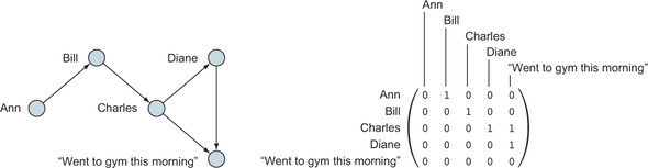
3.3.3. Adjacency matrix

Another way graph theorists represent graphs is by an adjacency matrix (see figure 3.15). It’s not the way GraphX represents graphs, but, separate from GraphX, Spark’s MLlib machine learning library has support for adjacency matrices and, more generally, sparse matrices. If you don’t need edge properties, you can sometimes find faster-performing algorithms in MLlib than in GraphX. For example, for a recommender system, strictly from a performance standpoint, mllib.recommendation.ALS can be a better choice than graphx.lib.SVDPlusPlus, although they are different algorithms with different behavior. SVDPlusPlus is covered in section 7.1.

Figure 3.15. A graph and its equivalent adjacency matrix. Notice that an adjacency matrix doesn’t have a place to put edge properties.

3.3.4. Graph querying systems

There are dozens of graph querying languages, but this section discusses three of the most popular ones and compares them to stock GraphX 1.6. Throughout, we use the example of “Tell me the friends of friends of Ann.”

SPARQL

SPARQL is a SQL-like language promoted by W3C for querying RDF graphs:

SELECT ?p
{
    "Ann" foaf:knows{2} ?p
}

Cypher

Cypher is the query language used in Neo4j, which is a property graph database.

MATCH (ann { name: 'Ann' })-[:knows*2..2]-(p)
RETURN p

Tinkerpop Gremlin

Tinkerpop is an attempt to create a standard interface to graph databases and processing systems—like the JDBC of graphs, but much more. There are several components to Tinkerpop, and Gremlin is the querying system. There is an effort, separate from the main Apache Spark project, to adapt Gremlin to GraphX. It’s called the Spark-Gremlin project, available on GitHub at https://github.com/kellrott/spark-gremlin. As of January 2015, the project status was “Nothing works yet.”

g.V("name", "ann").out('knows').aggregate(x).out('knows').except(x)

GraphX

GraphX has no query language out of the box as of Spark GraphX 1.6. The GraphX API is better suited to running algorithms over a large graph than to finding some specific information about a specific vertex and its immediate edges and vertices. Nevertheless, it is possible, though clunky:

val g2 = g.outerJoinVertices(g.aggregateMessages[Int](
  ctx => if (ctx.srcAttr == "Ann" && ctx.attr == "knows") ctx.sendToDst(1),
  math.max(_,_)))((vid, vname, d) => (vname, d.getOrElse(0)))
g2.outerJoinVertices(g2.aggregateMessages[Int](
  ctx => if (ctx.srcAttr._2 == 1 && ctx.attr == "knows") ctx.sendToDst(2),
  math.max(_,_)))((vid, vname, d) => (vname, d.getOrElse(0))).
  vertices.map(_._2).filter(_._2 == 2).map(_._1._1).collect

This is far too complex to dissect in this chapter, but by the end of part 2 of this book, this miniature program will make sense. The point is to illustrate that GraphX, as of version 1.6.0, does not have a quick and easy query language. Two things make the preceding code cumbersome: looking for a specific node in the graph and traversing the graph exactly two steps (as opposed to one step or, alternatively, an unlimited number of steps bound by some other condition).

There is some relief, though. In chapter 10 you’ll see GraphFrames, which is a library on GitHub that does provide a subset of Neo4j’s Cypher language, together with SQL from Spark SQL, to allow for fast and convenient querying of graphs.

3.4. Summary

• Doing GraphX has a lot of prerequisites: Scala, Spark, and graphs.
• Scala is an object-functional programming language that carries not only the functional philosophy, but also its own philosophy that includes conciseness and implementing features in its library rather than the language itself.
• Spark is effectively a distributed version of Scala, introducing the Resilient Distributed Dataset (RDD).
• GraphX is a layer on top of Spark for processing graphs.
• Graphs have their own vocabulary.
• GraphX supports property graphs.
• GraphX has no query language in the way that graph databases do.