Chapter 4. GraphX Basics

This chapter covers

• The basic GraphX classes
• The basic GraphX operations, based on Map/Reduce and Pregel
• Serialization to disk
• Stock graph generation

Now that we have covered the fundamentals of Spark and of graphs in general, we can put them together with GraphX. In this chapter you’ll use both the basic GraphX API and the alternative, and often better-performing, Pregel API. You’ll also read and write graphs, and for those times when you don’t have graph data handy, generate random graphs.

4.1. Vertex and edge classes

As discussed in chapter 3, Resilient Distributed Datasets (RDDs) are the fundamental building blocks of Spark programs, providing for both flexible, high--performance, data-parallel processing and fault-tolerance. The basic graph class in GraphX is called Graph, which contains two RDDs: one for edges and one for vertices (see figure 4.1).

Figure 4.1. A GraphX Graph object is composed of two RDDs: one for the vertices and one for the edges.

One of the big advantages of GraphX over other graph processing systems and graph databases is its ability to treat the underlying data structures as both a graph, using graph concepts and processing primitives, and also as separate collections of edges and vertices that can be mapped, joined, and transformed using data-parallel processing primitives.

In GraphX, it’s not necessary to “walk” a graph (starting from some vertex) to get to the edges and vertices you’re interested in. For example, transforming vertex property data can be done in one fell swoop in GraphX, whereas in other graph-processing systems and graph databases, such an operation can be contrived in terms of both the necessary query and how such a system goes about performing the operation.

You can construct a graph given two RDD collections: one for edges and one for vertices. Once the graph has been constructed, you can access these collections via the edges() and vertices() accessors of Graph.

Because Graph defines a property graph (as described in chapter 3), each edge and each vertex carries its own custom properties, described by user-defined classes.

In the UML diagram in figure 4.2, VD and ED serve as placeholders for these user-defined classes. Graph is a type-parameterized generic class Graph[VD,ED]. For example, if you had a graph showing cities and their population size as vertices connected by roads, one representation would be Graph[Long,Double], where the vertex data attribute is a Long type for the population size and the edge type a Double for the distance between cities.

Figure 4.2. UML diagram of GraphX’s Graph and its dependencies. Note that GraphX defines VertexId to be a type synonym of a 64-bit Long.

You always have to supply some type of class for VD or ED, even if it’s Int or String. It could be considered a slight limitation in GraphX that there is no inherent support for a “property-less” graph, because the closest you can come is to, for example, make Int the type parameter and set every edge and vertex to the same dummy value.

GraphX defines VertexId to be of type 64-bit Long. You have no choice in the matter. Notice that Edge contain VertexIds rather than references to the vertices (which are the (VertexId,VD) Scala Tuple2 pairs). That’s because graphs are distributed across the cluster and don’t reside within a single JVM, and an edge’s vertices may be physically residing on a different node in the cluster!

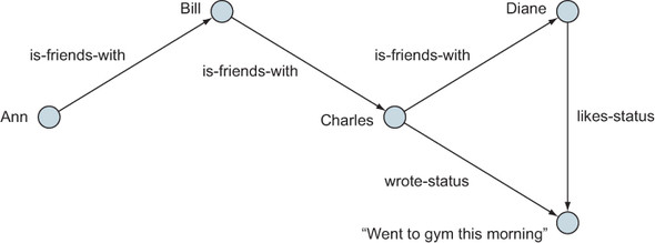
To construct a graph, we can call Graph() as if it were a constructor. The example in listing 4.1 (see page 65) constructs the same graph we saw in chapter 1. We’ll use this same graph (see figure 4.3) throughout this chapter in other examples.

Figure 4.3. Example graph to be constructed and used throughout this chapter

Listing 4.1. Construct a graph as shown in figure 4.3

import org.apache.spark.graphx._

val myVertices = sc.makeRDD(Array((1L, "Ann"), (2L, "Bill"),
 (3L, "Charles"), (4L, "Diane"), (5L, "Went to gym this morning")))

val myEdges = sc.makeRDD(Array(Edge(1L, 2L, "is-friends-with"),
 Edge(2L, 3L, "is-friends-with"), Edge(3L, 4L, "is-friends-with"),
 Edge(4L, 5L, "Likes-status"), Edge(3L, 5L, "Wrote-status")))

val myGraph = Graph(myVertices, myEdges)

myGraph.vertices.collect

res1: Array[(org.apache.spark.graphx.VertexId, String)] = Array((4,Diane),
(1,Ann), (3,Charles), (5,Went to gym this morning), (2,Bill))

Scala Tip

Using the Scala keyword object (as opposed to class) defines a singleton object. When such a singleton object has the same name as a class, it’s called a companion object. Graph from the GraphX API is an example of a class that has a companion object, and as shown in the sidebar, each has its own API. A companion object, besides being a place where apply() can be defined (for example, to implement the Factory pattern), is also a place where functions akin to Java static functions can be defined.

Scala Tip

When a Scala class or object has a method called apply(), the apply can be omitted. Thus, although Graph() looks like a constructor, it’s an invocation of the apply() method. This is an example of using Scala’s apply() to implement the Factory pattern described in the book Design Patterns by Gamma et al (Addison-Wesley Professional, 1994).

Spark Tip

In GraphX tutorials you’ll often see parallelize() instead of makeRDD(). They are synonyms. makeRDD() is your author Michael Malak’s personal preference because he feels it is more descriptive and specific.

Listing 4.1 constructed the graph that was shown in figure 4.3. You can also get the edges, as shown in the following listing.

Listing 4.2. Retrieve the edges from the just-constructed graph

myGraph.edges.collect

res2: Array[org.apache.spark.graphx.Edge[String]] = Array(Edge(1,2,
is-friends-with), Edge(2,3,is-friends-with), Edge(3,4,is-friends-with),
     Edge(3,5,Wrote-status), Edge(4,5,Likes-status))

Being regular (unordered) RDDs, the vertex and edge RDDs aren’t guaranteed any particular order.

You can also use the triplets() method to join together the vertices and edges based on VertexId. Although Graph natively stores its data as separate edge and vertex RDDs, triplets() is a convenience function that joins them together for you, as shown in the following listing.

Listing 4.3. Get a triplet(s) version of the graph data

myGraph.triplets.collect

res3: Array[org.apache.spark.graphx.EdgeTriplet[String,String]] =
Array(((1,Ann),(2,Bill),is-friends-with),
((2,Bill),(3,Charles),is-friends-with),
((3,Charles),(4,Diane),is-friends-with),
((3,Charles),(5,Went to gym this morning),Wrote-status),
((4,Diane),(5,Went to gym this morning),Likes-status))

The return type of triplets() is an RDD of EdgeTriplet[VD,ED], which is a subclass of Edge[ED] that also contains references to the source and destination vertices associated with the edge. As shown in figure 4.4, the EdgeTriplet gives access to the Edge (and the edge attribute data) as well as the vertex attribute data for the source and destination vertices. As you will see, having easy access to both the edge and vertex data makes many graph-processing tasks easier.

Figure 4.4. The triplets() method is a convenience function that allows easy access to both edge and vertex attributes.

Table 4.1 shows some of the useful fields available on EdgeTriplet.

Table 4.1. Key fields provided by EdgeTriplet

Field	Description
Attr	Attribute data for the edge
srcId	Vertex id of the edge’s source vertex
srcAttr	Attribute data for the edge’s source vertex
dstId	Vertex id of the edge’s destination vertex
dstAttr	Attribute data for the edge’s destination vertex

4.2. Mapping operations

The real meat of GraphX Map/Reduce operations is called aggregateMessages() (which supplants the deprecated mapReduceTriplets()), but to get our feet wet, let’s first look at the much simpler mapTriplets(). Doing so will also serve to introduce another important idea in GraphX. Many of the operations we’ll look at in this book return a new Graph that’s a transformation of the original Graph object. Though the end result might be the same as if we had transformed edges and vertices ourselves and created a new Graph, we won’t benefit from optimizations that GraphX provides under the covers.

4.2.1. Simple graph transformation

To the graph constructed in the previous section, let’s add an annotation to each “is-friends-with” edge whenever the person on the initiating side of the friendship has a name that contains the letter a. How will we add this annotation? By transforming the Edge type from String to a tuple (String, Boolean) as shown in the next listing. The EdgeTriplet class comes in handy here as we need access to both the edge attribute and the attribute for the source vertex.

Listing 4.4. Add Boolean annotation to edges indicating a condition

yGraph.mapTriplets(t => (t.attr, t.attr=="is-friends-with" &&
 t.srcAttr.toLowerCase.contains("a"))).triplets.collect

res4: Array[org.apache.spark.graphx.EdgeTriplet[String,(String, Boolean)]]
 = Array(((1,Ann),(2,Bill),(is-friends-with,true)),
((2,Bill),(3,Charles),(is-friends-with,false)),
((3,Charles),(4,Diane),(is-friends-with,true)),
((3,Charles),(5,Went to gym this morning),(Wrote-status,false)),
((4,Diane),(5,Went to gym this morning),(Likes-status,false)))

The resulting graph is shown in figure 4.5. Note that our original graph, myGraph (without the extra Boolean annotation on each edge), is still around. And, actually, the graph in the figure isn’t permanent in any sense of the word because we didn’t bother to capture it into a Scala val or var before handing it off immediately to triplets().

Figure 4.5. We opted to change the Edge type, compared to figure 4.3, as part of the way we invoked mapTriplets(). Whereas the Edge type was String in figure 4.3, this resulting graph’s Edge type is the Tuple2 of type (String,Boolean).

Although mapTriplets() can optionally take two parameters, here we used the first parameter, an anonymous function that takes as input an EdgeTriplet and returns as output our new Edge type of the Tuple2 of (String,Boolean).

Scala Tip

If you don’t declare the return type of an anonymous function, Scala will infer the type by the type of what you are returning. In the preceding example, if we wanted to ask the Scala compiler to double-check our intentions (as well as document the types to the human reader of our code), we could have instead written this:

myGraph.mapTriplets((t => (t.attr, t.attr=="is-friends-with" &&
                           t.srcAttr.toLowerCase.contains("a"))) :
                    (EdgeTriplet[String,String] =>
                       Tuple2[String,Boolean]) )
       .triplets.collect

There’s a similar mapVertices() API call that allows you to transform the Vertex class on the fly, similar to how mapTriplets() allows you to change the Edge class. You can explore mapVertices() on your own.

4.2.2. Map/Reduce

Many graph processing tasks involve aggregating information from around the local neighborhood of a vertex. By neighborhood we mean the associated edges and vertices around a vertex. You’ll see examples of aggregating information from the local neighborhood in the next chapter when we look at some of the classic graph algorithms, such as triangle counting.

Definition

A triangle occurs when one vertex is connected to two other vertices and those two vertices are also connected. In a social media graph showing which people are friends, a triangle occurs when people who are my friends are also friends with each other. We could say that how many triangles a person is involved with gives a sense of how connected the community is around that person.

To identify whether a vertex is part of a triangle, you need to consider the set of edges that connect to that vertex, the set of vertices at the other end of those edges, and whether any of the associated vertices also have an edge between them. For each vertex this involves considering information in its neighborhood.

We’ll leave triangle counting to the next chapter and look at a simpler example that will allow us to concentrate on some of the key concepts underlying processing and aggregating information from the neighborhood of a vertex. This idea has strong parallels with the classic Map/Reduce paradigm (see chapter 1). Much like in Map/Reduce, we’ll define transformations (map) that are applied to individual structures in the neighborhood of the vertex. Then the output from those transformations will be merged to update the vertex information (reduce).

Our example will count the out-degree of each vertex—for each vertex, the count of edges leaving the vertex. To do this we’ll process each vertex indirectly by acting on the edges and their associated source and destination vertices. Rather than explicitly counting edges coming out of each vertex we’ll get the edges to “emit” a message to the relevant source vertex, which amounts to the same thing. Aggregating these messages gives us the answer we want.

The following listing uses the aggregateMessages() method and is all we need to carry out this task in GraphX.

Listing 4.5. Using aggregateMessages[]() to compute the out-degree of each vertex

myGraph.aggregateMessages[Int](_.sendToSrc(1), _ + _).collect

res5: Array[(org.apache.spark.graphx.VertexId, Int)] = Array((4,1), (1,1),
(3,2), (2,1))

The array returned contains pairs (Tuple2s) that show us the ID of the vertex and the vertex’s out-degree. Vertex #4 has only one outgoing edge, but vertex #3 has two.

How did it do that? To understand what this code is doing, we’ll break it down into its constituent parts. First here’s the method signature for aggregateMessages:

def aggregateMessages[Msg](
    sendMsg: EdgeContext[VD, ED, Msg] => Unit,
    mergeMsg: (Msg, Msg) => Msg)
  : VertexRDD[Msg]

The first thing to note is the type parameterization of the method: Msg (short for message, and you’ll see why in a moment). The Msg type represents the answer we want to generate; in this case, we want a count of edges emanating from a vertex, so Int is the appropriate type to parameterize aggregateMessages.

Scala Tip

With all the type inference the Scala compiler does for you, you might expect it to be able to infer the type parameter for aggregate-Messages[]() based on the return type of the anonymous function it takes as its first parameter. After all, they’re both declared as type Msg in the function declaration for aggregateMessages[](). The reason the Scala compiler can’t infer the type in this case is because Scala is a left-to-right compiler, and the anonymous function appears (slightly) later in the source code than the name of the function you’re invoking.

The two parameters to aggregateMessages, sendMsg and mergeMsg, provide the transformation and reduce logic.

sendMsg

sendMsg is a method that takes an EdgeContext as parameter and returns nothing (recall from earlier chapters that Unit is the Scala equivalent of Java’s void). EdgeContext is a type-parameterized class similar to EdgeTriplet. EdgeContext contains the same fields as EdgeTriplet but also provides two additional methods for message sending:

• sendToSrc —Sends a message of type Msg to the source vertex.
• sendToDst —Sends a message of type Msg to the destination vertex.

These two methods are the key to how aggregateMessages works. A message is nothing more than a piece of data sent to a vertex. For each edge in the graph, we can choose to send a message to either the source or the destination vertex (or both). Inside the sendMsg method the EdgeContext parameter can be used to inspect the values of the edge attributes and the source and destination vertices as part of the logic. For our example, we’re counting how many edges exit from a vertex, so we’ll send a message containing the integer 1 to the source vertex.

mergeMsg

All the messages for each vertex are collected together and delivered to the mergeMsg method. This method defines how all the messages for the vertex are reduced down to the answer we’re looking for. In the example code, we want to sum each 1 that’s sent to the source vertex to find the total number of outgoing edges. That is what the _ anonymous function using + does.

The result of applying mergeMsg for each of the vertices is returned as a VertexRDD[Int]. VertexRDD is an RDD containing Tuple2s consisting of the VertexId and the mergeMsg result for that vertex. One thing to notice is that since vertex #5 didn’t have any outgoing edges, it won’t receive any messages and therefore doesn’t appear in the resulting VertexRDD.

Cleaning up the results

Interpreting these raw VertexIds is inconvenient, so let’s join with the original vertices to get the human-readable names. In the following listing we use Spark RDD join(), which is a method from PairRDDFunctions.

Listing 4.6. RDD join() to match up VertexIds with vertex data

myGraph.aggregateMessages[Int](_.sendToSrc(1),
 _ + _).join(myGraph.vertices).collect

res6: Array[(org.apache.spark.graphx.VertexId, (Int, String))] =
Array((4,(1,Diane)), (1,(1,Ann)), (3,(2,Charles)), (2,(1,Bill))

Spark Tip

Whenever you have an RDD of Tuple2, Spark provides an automatic conversion when needed from RDD[] to PairRDDFunctions[] under the assumption that the Tuple2 is a key/value pair (K,V). join() is one of many functions that become available for RDD[Tuple2]s. The conversion is automatically available in the REPL, but in a compiled Scala program you need to import org.apache.spark.SparkContext._ (in addition to the regular import org.apache.spark.SparkContext).

Well, that’s a little verbose. We don’t need those VertexIds anymore, so we can get rid of them by using the map() method of RDD. Then we can use the swap() method of Tuple2 to swap the order within each pair so that the human-readable vertex name appears before its out-degree numerical value, for the purposes of providing pretty output, as shown in the following listing.

Listing 4.7. map() and swap() to clean up output

myGraph.aggregateMessages[Int](_.sendToSrc(1),
 _ + _).join(myGraph.vertices).map(_._2.swap).collect

res7: Array[(String, Int)] = Array((Diane,1), (Ann,1), (Charles,2),
(Bill,1))

Now for some final mopping up. How can we get back that missing vertex #5? By using rightOuterJoin() instead of join(), as shown in the following listing.

Listing 4.8. rightOuterJoin() instead of join() to pull in “forgotten” vertices

myGraph.aggregateMessages[Int](_.sendToSrc(1),
 _ + _).rightOuterJoin(myGraph.vertices).map(_._2.swap).collect

res8: Array[(String, Option[Int])] = Array((Diane,Some(1)), (Ann,Some(1)),
 (Charles,Some(2)), (Went to gym this morning,None), (Bill,Some(1)))

Ugh! What is all that Some and None stuff? Well, outer joins can give null or empty fields when there’s no corresponding record in the joining table. It’s Scala’s way of avoiding problems with null (though it still does have null for when you need it, and often there’s no way around it when you need to interface with Java code). Some and None are values from Scala’s Option[], and to get rid of them we can use the getOrElse() method from Option[]. In the process, we have to dig inside our Tuple2, so we won’t be able to use the convenience of swap() anymore, as shown in the following listing.

Listing 4.9. Option[]’s getOrElse() to clean up rightOuterJoin() output

myGraph.aggregateMessages[Int](_.sendToSrc(1),
 _ + _).rightOuterJoin(myGraph.vertices).map(
 x => (x._2._2, x._2._1.getOrElse(0))).collect

res9: Array[(String, Int)] = Array((Diane,1), (Ann,1), (Charles,2), (Went to
     gym this morning,0), (Bill,1))

Spark Tip

Using Option[] instead of null in Scala opens up a world of possibilities for more functional programming because Option[] can be considered a mini-collection (containing either zero or one element). Functional programming constructs such as flatmap(), for comprehensions and partial functions, can be used on Option[]s, whereas they can’t be used on nulls.

4.2.3. Iterated Map/Reduce

Most algorithms involve more than a single step or iteration. aggregateMessages can be used to implement algorithms where we continuously update each vertex based only on information obtained from neighboring edges and vertices.

To see this idea in action, we’ll implement an algorithm that finds the vertex with the greatest distance from its ancestor in the graph. At the end of the algorithm we hope to have each vertex labeled with the farthest distance from an ancestor.

We’ll assume our graphs don’t have cycles (cycles occur when we have edges that go around from one vertex and eventually loop back to the same vertex). Dealing with cyclic graphs usually makes for added complexity in our algorithms, and we’ll show you some strategies for dealing with those later on.

First we define the sendMsg and mergeMsg functions that will be called by aggregateMessages. We define them up front rather than as anonymous functions in the body of the aggregate messages function, as sometimes the code can become a little cluttered.

The common way to express iteration in functional programming is through recursion, so next we’ll define a helper recursive function, propagateEdgeCount, which will continuously call aggregateMessages (see the following listing).

Listing 4.10. Iterated (via recursion) Map/Reduce to find distance of furthest vertex

In this listing, propagateEdgeCount() adds 1 to the distance traveled so far and sends that to the destination vertex of each edge. The destination vertex then does a max() across all the distance messages it receives and makes that the new distance for itself.

An important point to note is that we define when to stop the recursion by comparing the original graph and the updated graph after each iteration. When there’s no difference between the graphs, we stop. Note that the reduce(_ + _) check works because we know that the new distance between vertices must be at least as big as the old distance and therefore the difference must be non-negative; we can’t have a situation where we add a negative to a positive and get a zero that way.

Tip

Alternatively, for better performance, we could avoid doing the join() completely by adding another vertex property—a Boolean that indicates whether the value has been updated. Then we can reduce() on that Boolean and not involve the VertexRDD from the previous iteration in our recursion exit condition.

Now we have the recursive pump primed, we need to invoke it. We’ll feed in our myGraph graph, but first we need to initialize it. This is a key question for any iterative algorithm: how do we start? We need to think of the task in terms of what information we know for each vertex at the start and what answer we’ll want at the end. We’re looking for an integer value that tells us the farthest distance we would have to travel. At the start we have no idea about the distance, so we’ll set each vertex to zero and have the algorithm gradually diffuse new information across the graph:

val initialGraph = myGraph.mapVertices((_,_) => 0)
propagateEdgeCount(initialGraph).vertices.collect

res10: Array[(org.apache.spark.graphx.VertexId, Int)] = Array( (1,0), (2,1)),
     (3,2), (4,3), (5,4) )

Vertex #5 has the longest distance to an ancestor vertex, which is a distance of 4.

You’ve seen how quick it is to implement an iterative algorithm. The key point is to think how information (“messages”) can be delivered across edges and accumulated to reach the answer you’re looking for.

4.3. Serialization/deserialization

You saw how to read in edge pairs in chapter 2 using GraphX’s GraphLoader API. But that data had neither vertex properties nor edge properties, and one of the main advantages of GraphX is that it handles property graphs. Here we provide some custom code to read and write property graphs in binary and JSON formats. The RDF format, a standard format for graphs of “triples” (not property graphs), is shown in chapter 8.

4.3.1. Reading/writing binary format

In this section, we read and write a standard Hadoop sequence file, which is a binary file containing a sequence of serialized objects. The Spark RDD API function saveAsObjectFile() saves to a Hadoop sequence file, relying upon standard Java serialization to serialize the vertex and edge objects, as shown in the following listing.

Listing 4.11. Round-trip persisting to and reading from file

Spark Tip

Despite its name, saveAsObjectFile() saves to multiple files in a directory, with one file per Spark partition inside that directory. The parameter you pass in is the name of that directory.

Although our simple graph uses String as the vertex and edge property classes, because the preceding technique uses Java Serializable, it generalizes to handle any complex class you might want to attach to vertices or edges. Substitute the class name for String in the type parameter for objectFile[]().

The preceding code doesn’t specify a file system, so it saves to the local file system. In a real Spark cluster, prepend the destination directory name with the appropriate URI prefix; for example, hdfs://localhost:8020/myGraphVertices.

Saving to a single file: the cheater way

To avoid the multiple part files when saving to HDFS or S3 using saveAsObjectFile(), you can cheat by adding a coalesce(1,true), such as the following:

myGraph.vertices.coalesce(1,true).saveAsObjectFile("myGraphVertices")

The downside of this trick is that the entire RDD has to fit inside a single partition, meaning it has to fit inside a single executor. That’s fine for experimenting with small graphs, but not in production with big graphs.

Saving to a single file: the right way

Assuming you’re working in HDFS, the right way to produce a single file is to first allow Spark to create the part files (which it does in parallel) and then, as a second step, merge them into a single file. There are two ways to do this: at the command line or through the Hadoop Java API.

For the following example, first make sure you’re saving to HDFS rather than the local file system. The following URL assumes use of the Cloudera Quickstart VM; it will be different for other environments:

myGraph.vertices.saveAsObjectFile(
  "hdfs://localhost:8020/user/cloudera/myGraphVertices")

To merge the part files contained in the myGraphVertices directory, one option is to use the command line, which reads the HDFS part files and creates a single file on the local file system:

hadoop fs -getmerge /user/cloudera/myGraphVertices myGraphVerticesFile

The API equivalent to getmerge is called copyMerge(), which has the option for the destination to be HDFS, as shown in the following listing.

Listing 4.12. Saving to a single file in HDFS using the Hadoop Java API

import org.apache.hadoop.fs.{FileSystem, FileUtil, Path}
val conf = new org.apache.hadoop.conf.Configuration
conf.set("fs.defaultFS", "hdfs://localhost")
val fs = FileSystem.get(conf)
FileUtil.copyMerge(fs, new Path("/user/cloudera/myGraphVertices/"),
  fs, new Path("/user/cloudera/myGraphVerticesFile"), false, conf, null)

Scala Tip

You can combine multiple imports from the same package on the same line by enclosing the multiple class names in curly braces.

You’re still stuck with two files: one for vertices produced by the preceding code, and one for edges (created similarly). To truly create a single file, you can choose to persist the triplets instead with graph.triplets.saveAsObjectFile(), but note that this would be a wastel of disk space because full vertex data would be repeated for every edge that uses that vertex. In this example, saving triplets to a single file would take about 20 times as much disk space as saving the edges and vertices separately in two files.

If you’re using S3 instead of HDFS, the hadoop fs -getMerge command line and the Hadoop API copyMerge() won’t work. There are various shell scripts and GUI-based tools found on the Web that accomplish the same thing for S3.

4.3.2. JSON format

If you prefer to serialize to a human-readable format, you can use a JSON library. In the realm of Scala for JSON, wrappers around the venerable Jackson library for Java are popular. The wrapper Jerkson was popular until it was abandoned in 2012. In its place, Jackson has since released jackson-module-scala. Its syntax is not as concise as most Scala libraries, but it works. Although Jackson is already available in the Spark REPL, we need to do the following in listing 4.13 at the OS command line to make jackson-module-scala also available there.

Listing 4.13. Command line commands to use jackson-module-scala in the REPL

wget http://repo1.maven.org/maven2/com/fasterxml/jackson/module/
 jackson-module-scala_2.10/2.4.4/jackson-module-scala_2.10-2.4.4.jar
wget http://repo1.maven.org/maven2/com/google/guava/guava/14.0.1/
 guava-14.0.1.jar
./spark-shell --jars jackson-module-scala_2.10-2.4.4.jar,guava-14.0.1.jar

Note that the version numbers given (Scala 2.10 and Jackson 2.4.4, and its dependency Guava 14.0.1) are specific to Spark 1.6. If you’re using a different version of Spark, find out which version of Scala it’s using from the banner when you start up the REPL and which version of Jackson and Guava it’s using from the Maven pom.xml. In Spark 1.6, the version numbers of all the dependent jars are centralized into the root pom.xml in the Spark source tree. The version of jackson-module-scala has to match the version of Jackson that Spark is built with.

First we look at how to use Jackson to serialize the graph to JSON using the features of Spark we’ve looked at so far. Then we introduce a new feature, mapPartitions, which can give significant performance improvement in some situations.

Once you have the REPL set up, go ahead and once again create myGraph as in listing 4.1. Then you might naively serialize to JSON, as shown in the following listing.

Listing 4.14. Naïve approach to serialize to JSON

myGraph.vertices.map(x => {
    val mapper = new com.fasterxml.jackson.databind.ObjectMapper()
    mapper.registerModule(
        com.fasterxml.jackson.module.scala.DefaultScalaModule)
    val writer = new java.io.StringWriter()
    mapper.writeValue(writer, x)
    writer.toString
}).coalesce(1,true).saveAsTextFile("myGraphVertices")

Note

The output file is itself not JSON-compliant; rather, each line within the file is valid JSON. This is more conducive to distributed storage and distributed processing than trying to put commas at the end of every line except for the last line and putting open and close brackets at the beginning and end of the file.

Notice that for every vertex, we’re constructing an entirely new JSON parser! For such purposes, the Spark API provides an alternative to map() called mapPartitions(). This is what we do in the better performing version in listing 4.15.

Spark Tip

Whenever you have heavyweight initialization that should be done once for many RDD elements rather than once per RDD element, and if this initialization, such as creation of objects from a third-party library, cannot be serialized (so that Spark can transmit it across the cluster to the worker nodes), use mapPartitions() instead of map(). mapPartitions() provides for the initialization to be done once per worker task/thread/partition instead of once per RDD data element.

Listing 4.15. Better performing way to serialize/deserialize to/from JSON

import com.fasterxml.jackson.core.`type`.TypeReference
import com.fasterxml.jackson.module.scala.DefaultScalaModule

myGraph.vertices.map(x => {
    val mapper = new com.fasterxml.jackson.databind.ObjectMapper()
    mapper.registerModule(
        com.fasterxml.jackson.module.scala.DefaultScalaModule)
    val writer = new java.io.StringWriter()
    mapper.writeValue(writer, x)
    writer.toString
}).coalesce(1,true).saveAsTextFile("myGraphVertices")

myGraph.vertices.mapPartitions(vertices => {
    val mapper = new com.fasterxml.jackson.databind.ObjectMapper()

    mapper.registerModule(DefaultScalaModule)
    val writer = new java.io.StringWriter()
    vertices.map(v => {writer.getBuffer.setLength(0)
                       mapper.writeValue(writer, v)
                       writer.toString})
}).coalesce(1,true).saveAsTextFile("myGraphVertices")

myGraph.edges.mapPartitions(edges => {
    val mapper = new com.fasterxml.jackson.databind.ObjectMapper();
    mapper.registerModule(DefaultScalaModule)
    val writer = new java.io.StringWriter()
    edges.map(e => {writer.getBuffer.setLength(0)
                    mapper.writeValue(writer, e)
                    writer.toString})
}).coalesce(1,true).saveAsTextFile("myGraphEdges")

val myGraph2 = Graph(
    sc.textFile("myGraphVertices").mapPartitions(vertices => {
        val mapper = new com.fasterxml.jackson.databind.ObjectMapper()
        mapper.registerModule(DefaultScalaModule)
        vertices.map(v => {
            val r = mapper.readValue[Tuple2[Integer,String]](v,
                new TypeReference[Tuple2[Integer,String]]{})
            (r._1.toLong, r._2)
        })
    }),
    sc.textFile("myGraphEdges").mapPartitions(edges => {
        val mapper = new com.fasterxml.jackson.databind.ObjectMapper()
        mapper.registerModule(DefaultScalaModule)
        edges.map(e => mapper.readValue[Edge[String]](e,
            new TypeReference[Edge[String]]{}))
    })
)

Scala Tip

If you need to use a reserved Scala keyword, surround it with a backtick on either side (`—also known as the grave accent character). This comes up often when using Java libraries in Scala.

Notice that due to a weakness in Jackson, we had to read in the vertex IDs as Integers and then convert them to Longs. This limits vertex IDs to the 2 billion range. Also notice that Jackson made us repeat the vertex and edge property class type parameters (String, in this case) twice each for readValue[](), so if you use a custom class, replace it in both places. Finally, as with the binary example, when using a distributed file system, remember to eliminate the coalesce(1,true).

4.3.3. GEXF format for Gephi visualization software

Gephi is a powerful open source graph visualization tool, and GEXF is its native XML format. In this section, we serialize to .gexf, as shown in the following listing and in figure 4.6. Gephi is open source and free to download from gephi.github.io. Its use is described in appendix B.

Figure 4.6. The generated .gexf file loaded into Gephi

Listing 4.16. Export to GEXF for Gephi visualization software

def toGexf[VD,ED](g:Graph[VD,ED]) =
    "<?xml version="1.0" encoding="UTF-8"?>
" +
    "<gexf xmlns="http://www.gexf.net/1.2draft" version="1.2">
" +
    "  <graph mode="static" defaultedgetype="directed">
" +
    "    <nodes>
" +
    g.vertices.map(v => "      <node id="" + v._1 + "" label="" +
                        v._2 + "" />
").collect.mkString +
    "    </nodes>
" +
    "    <edges>
" +
    g.edges.map(e => "      <edge source="" + e.srcId +
                     "" target="" + e.dstId + "" label="" + e.attr +
                     "" />
").collect.mkString +
    "    </edges>
" +
    "  </graph>
" +
    "</gexf>"

val pw = new java.io.PrintWriter("myGraph.gexf")
pw.write(toGexf(myGraph))
pw.close

Scala Tip

Sometimes the REPL gets confused about when you want to continue a line of code to the next line, such as when you end a line on a plus sign for string concatenation. In those cases, enter paste mode by entering the command :paste. Exit paste mode by pressing Ctrl-D.

4.4. Graph generation

If you don’t have graph data available, the GraphGenerators object can generate some random graphs for you. This approach can be useful when you need to test out some ideas about a graph function or an algorithm and you need to get something working quickly. One of them, generateRandomEdges(), is a helper function for the main graph-generating functions; it’s not that useful on its own because it takes as a parameter a single vertex ID from which all the generated edges will emanate. But let’s take a look at the four full graph generators that are available in Spark 1.6.

4.4.1. Deterministic graphs

The first two graph structures we cover are non-random: the grid and the star. The following listings assume you’ve already done import org.apache.spark.graphx._. For example, util.GraphGenerators refers to org.apache.spark.graphx.util.GraphGenerators.

Grid graph

A grid graph has a specific configuration of vertices and edges that are laid out as if in a 2-D grid or matrix. Each vertex is labeled with the row and column of its position in the grid (for example, the top left vertex is labeled (0,0)). Then each vertex is connected to its neighbor immediately above, below, left, and right. The following listing demonstrates how to create a 4x4 grid graph. The layout of the graph is show in figure 4.7.

Figure 4.7. A generated gridGraph() visualized in Gephi. There is no randomness to a grid graph; the grid is always complete.

Listing 4.17. Generate a grid graph

val pw = new java.io.PrintWriter("gridGraph.gexf")
pw.write(toGexf(util.GraphGenerators.gridGraph(sc, 4, 4)))
pw.close

Star graph

A star graph has one vertex connected by edges to all other vertices—there are no other edges in the graph. As figure 4.8 shows, the name comes from its star-like layout.

Figure 4.8. A generated starGraph() visualized in Gephi. Like gridGraph(), it is not random.

The graph is generated by calling GraphGenerators.starGraph with the number of vertices as the second parameter to the method. Vertex 0 is always the center of the star, so the call GraphGenerators.starGraph(sc, 8) in the following listing results in a graph with Vertex 0 connected to 7 other vertices.

Listing 4.18. Generate a star graph

val pw = new java.io.PrintWriter("starGraph.gexf")
pw.write(toGexf(util.GraphGenerators.starGraph(sc, 8)))
pw.close

4.4.2. Random graphs

GraphX provides two ways to generate graphs randomly: a single-step algorithm (called log normal) that attaches a particular number of edges to each vertex, and a multistep procedural algorithm (called R-MAT) that generates graphs that are closer to what is found in the real world.

Degree-based: log normal graph

The log normal graph focuses on the out-degrees of the vertices in the graphs it generates. It ensures that if you take a histogram of all the out-degrees, they form a log normal graph, which means that log(d) forms a normal distribution (Gaussian bell shape), where the ds are the vertex degrees. The following listing incorporates the code from listing 4.5 that counted the out-degrees, and as you can see, there are a lot of vertices of degree 6, with it tailing off to the left (lower-degree vertices) and a longer tail to the right (higher-degree vertices). Figure 4.9 shows a possible output graph.

Figure 4.9. A generated logNormalGraph() visualized in Gephi. The only constraint in logNormalGraph() is the out-degree of each vertex, and otherwise there are no restrictions on where edges are placed. Some edges have the same source and destination vertices. And some pairs of vertices have multiple parallel edges, represented in the Gephi visualization (which does not render parallel edges directly) by darker edges and larger arrowheads.

Listing 4.19. Generate a log normal graph

Procedural-based: R-MAT graph

R-MAT, which stands for recursive matrix, is intended to simulate the structure of typical social networks. As opposed to the “degree-based” approach of the earlier logNormalGraph(), rmatGraph() takes a “procedural” approach. It adds edges one at a time into quadrants of the graph (and quadrants within quadrants, and so on), based on predetermined probabilities for each quadrant, as shown in the following listing. A possible output graph is shown in figure 4.10.

Figure 4.10. rmatGraph’s recursive quadrant subdivision leaves some relative loner vertices and also makes for some groups of vertices having a high number of interconnections.

Listing 4.20. Generate an R-MAT graph

rmatGraph assumes the number of vertices passed in as a parameter is a power of 2. If it’s not, rmatGraph rounds it up to the next power of 2 for you. It needs the number of vertices to be a power of 2 for the recursive quadrant subdivision, as shown in figure 4.11. rmatGraph starts out by laying the vertices out in a grid (the non-grid layout in figure 4.10 is caused by Gephi trying to make the resultant graph look nice) and then randomly places edges one by one, choosing vertices based on probabilities arising from the recursive quadrants. Some vertices may by chance end up with zero edges, which is why the Gephi rendering in figure 4.10 shows only 16 vertices, even though listing 4.20 specifies 32 vertices.

Figure 4.11. Recursive quadrants from the 2004 paper “R-MAT: A Recursive Model for Graph Mining” by Chakrabarti et al. GraphX uses the hard-coded probabilities a=0.45, b=0.15, c=0.15, d=0.25.

4.5. Pregel API

Section 2.3 states that complete algorithms can be built by repeated application of aggregateMessages. This is such a common requirement that GraphX provides an API based on Google’s Pregel to accomplish such iterative algorithms in a concise manner. It is so concise that an entire algorithm can be expressed with a single Pregel call. In fact, many of GraphX’s pre-canned algorithms are implemented in terms of a single Pregel call.

GraphX’s Pregel API provides a concise functional approach to algorithm design. It also provides some performance benefits through caching and uncaching intermediate data sets; getting this right is generally tricky for programmers and relieves them of the burden of having to deal with low-level performance tuning.

In GraphX the implementation of Pregel is a form of Bulk Synchronous Parallel (BSP) processing. As its name suggests, BSP is a parallel processing model developed in the 1980s. BSP is not specifically designed for graph processing, but when Google implemented its graph processing framework, Pregel, it used the principles behind BSP. Google’s Pregel is the inspiration for Spark’s own Pregel API.

As shown in figure 4.12, the algorithm is decomposed into a series of supersteps, with each superstep being a single iteration. Within each superstep, per-vertex calculations can be performed in parallel. At the end of the superstep, each vertex generates messages for other vertices that are delivered in the next superstep. Due to the synchronization barrier, nothing from a subsequent superstep gets executed until the current superstep is fully completed. Unlike some general purpose, low-level libraries for distributed high-performance computing, the synchronization in the Pregel API is handled automatically for you by GraphX.

Figure 4.12. BSP allows processing in parallel within a superstep. Messages are then generated and delivered for the next superstep. The next superstep does not begin until the current superstep is completed and all messages are delivered to the next superstep. This is illustrated by the synchronization barriers.

One of the benefits of having a framework like this is that it’s useful to have a high-level abstraction that lets you specify program behavior that can then be efficiently parallelized by the framework.

Figure 4.13 shows how the Pregel API processes a single superstep in more detail. The messages sent in the previous superstep are grouped together by vertex and processed by a “merge message” (mergeMsg) function so that each vertex is associated with a single merged message (unless the vertex wasn’t sent any messages). The mergeMsg function works in exactly the same way as the mergeMsg function used by aggregateMessages: it must be commutative and associative so that it can repeatedly process pairs of messages to arrive at a single result for each vertex.

Figure 4.13. Messages for a vertex from the previous superstep are processed by the mergeMsg and vprog functions to update the vertex data. The vertex then sends messages to be delivered in the next superstep.

Unlike aggregateMessages, though, the result of mergeMsg doesn’t update the vertex directly but is passed to a vertex program that takes a vertex (both the VertexID and the data) and the message as input and returns new vertex data that’s applied by the framework to the vertex.

In the last step of the superstep iteration, each vertex gets to send a message along each of its out-edges. The vertex can also choose not to send a message; if the destination vertex doesn’t receive any messages from its source vertices, it will no longer be considered for processing in the next superstep. The logic for this decision is encapsulated in a sendMsg function. Figure 4.14 shows the complete flow of the Pregel method call.

Figure 4.14. Flow of GraphX Pregel API

Now that you have an idea of how this works, let’s see what the Pregel method signature looks like:

def pregel[A]
      (initialMsg: A,
       maxIter: Int = Int.MaxValue,
       activeDir: EdgeDirection = EdgeDirection.Out)
      (vprog: (VertexId, VD, A) => VD,
       sendMsg: EdgeTriplet[VD, ED] => Iterator[(VertexId, A)],
       mergeMsg: (A, A) => A)
    : Graph[VD, ED]

As with aggregateMessages, the method is type-parameterized by the message (A) that will be received and delivered by each vertex. Unlike aggregateMessages, though, pregel does some extra work for you by returning a new Graph object rather than a VertexRDD.

Scala Tip

Notice that the function has two sets of parameters. In Scala you can split parameters up into multiple parameter lists. You can invoke the function by providing all the parameters, although you have to use the syntax of surrounding each list of parameters in its own set of parentheses. This is how we call pregel in the upcoming example. Alternatively, you can use partial function application. For example, you could do val p = Pregel(g,0)_ (note the underscore is required when using partial application). Then at some later point, you could do p(myVprog, mySendMsg, myMergeMsg). Later still, you could reuse p again for some other similar Pregel invocation.

The first set of parameters defines some settings or algorithm parameters. initialMsg is a value that will be delivered to the vertex to kick-start the processing. Often this is some sort of zero value that represents our lack of knowledge at the beginning of the algorithm.

maxIter defines how many iterations or supersteps will be carried out. Some algorithms have convergence guarantees that ensure an accurate answer will be reached within a reasonable number of iterations. But many algorithms don’t give this guarantee, giving rise to the possibility that the algorithm will continue forever. In this latter case, it’s definitely a good idea to specify a number smaller than the default Int.MaxValue!

The second set of parameters defines the three functions already outlined: vprog, sendMsg, and mergeMsg. These define the behavior we want to encode into the algorithm. The introduction to this section mentioned that Pregel provides similar functionality to the iterated MapReduce using aggregateMessages. There are some subtle differences between the two that we will call out here.

First, aggregateMessages only requires two functions to define its behavior: sendMsg and mergeMsg. What’s the purpose of this vertex program, vprog? It provides greater flexibility in defining the logic. In some cases, the message and the vertex data type are the same, and only some simple logic is required to update the graph with a new value.

In other cases, the message and the vertex data will be different types. An example is the implementation of LabelPropagation, discussed in detail in the next chapter. LabelPropagation returns a Graph whose vertex data is a VertexId, but the message type is a Map relating VertexIDs to Long – Map[VertexId, Long]. The Map message passed to the vertex program is interrogated to find the VertexId with the highest Long value, and this is the ID that is used to update the vertex data.

The other key difference is the form of the sendMsg function signature, compared in table 4.2. Recall that EdgeTriplet contains information on an edge and its two vertex endpoints. EdgeContext adds two additional methods, sendToSrc and sendToDst.

Table 4.2. sendMsg function signature in aggregateMessages and Pregel

aggregateMessages	Pregel
EdgeContext[VD, ED, Msg] => Unit	EdgeTriplet[VD, ED] => Iterator[(VertexId, A)]

You may ask why there is this difference. The answer is that Pregel still relies on the deprecated mapReduceTriplets method to do its work and hasn’t been updated to use aggregateMessages. The work to implement Pregel using aggregateMessages is being tracked in SPARK-5062.

The following listing shows the iterated MapReduce example of listing 4.10, converted to Pregel.

Listing 4.21. Pregel to find distance of furthest vertex

val g = Pregel(myGraph.mapVertices((vid,vd) => 0), 0,
               activeDirection = EdgeDirection.Out)(
               (id:VertexId,vd:Int,a:Int) => math.max(vd,a),
               (et:EdgeTriplet[Int,String]) =>
                    Iterator((et.dstId, et.srcAttr+1)),
               (a:Int,b:Int) => math.max(a,b))
g.vertices.collect

res12: Array[(org.apache.spark.graphx.VertexId, Int)] = Array((4,3), (1,0),
(3,2), (5,4), (2,1))

Scala Tip

You always have the option of using named parameters. Sometimes this can make the code easier to read. Other times, if there are several parameters with default values, some such parameters can be skipped if in your function invocation you use named parameters for the later parameters.

The terminating condition for Pregel is that there are no more messages to be sent. In each iteration, if an edge’s vertices did not receive messages from the previous iteration, sendMsg will not be called for that edge. The activeDirection parameter to Pregel specifies this filter. For an edge with vertices srcId and destId,

• EdgeDirection.Out —sendMsg gets called if srcId received a message during the previous iteration, meaning this edge is considered an “out-edge” of srcId.
• EdgeDirection.In —sendMsg gets called if dstId received a message during the previous iteration, meaning this edge is considered an “in-edge” of dstId.
• EdgeDirection.Either —sendMsg gets called if either srcId or dstId received a message during the previous iteration.
• EdgeDirection.Both —sendMsg gets called if both srcId and dstId received messages during the previous iteration.

In the vertex distance example, we used EdgeDirection.Out because the vertex distance algorithm follows the edge directions of the graph. Once it reaches the “end” of the directed graph, it terminates.

If the graph has cycles, we have to be more careful because we’re likely to run into situations where a group of vertices continuously sends and receives messages without termination. One thing we can do to deal with this situation is use the maxIterations parameter to ensure that our algorithm terminates in a reasonable amount of time.

Another approach is to try and detect situations where the algorithm is looping around and not doing any useful new work. For example, the ShortestPaths algorithm discussed in the next chapter progressively updates a map with vertices reachable from the current vertex. The sendMsg function only issues messages if there’s new information to be added to the map that wouldn’t have already been seen by the message target.

4.6. Summary

• Pregel and its little sibling aggregateMessages() are the cornerstones of graph processing in GraphX.
• Most of the canned algorithms that come with GraphX are implemented in terms of Pregel.
• Because the terminating condition for Pregel is that no messages happen to be sent, algorithms that require more flexibility for the terminating condition have to be implemented using aggregateMessages() instead.
• Because GraphX doesn’t have built-in API functions to read and write property graphs (only to read in an edge list), we showed code to do that.
• If you don’t have data to work with, the GraphX API provides ways to generate both random and deterministic graphs.