CHAPTER 31
Six Sigma and Project Management

RIP STAUFFER, SENIOR CONSULTANT, WOODSIDE QUALITY SOLUTIONS

In general, Six Sigma is a data-driven, project-based, team-driven, and customer-focused methodology for achieving breakthrough levels of performance in strategically important processes. Six Sigma is essentially a quality initiative, in the vein of Total Quality Management (TQM), Lean Manufacturing, Business Process Reengineering (BPR), Statistical Process Control (SPC), and Continuous Improvement (CI). Many of these other process quality initiatives focus largely on the ongoing management and control of processes; many of the actions taken for improvement tend to be relatively quick turnaround, “just-do-it” reactions to emergent signals from the process. (For further discussion of some of these quality initiatives, see Chapter 11A.)

It’s worth noting that although Six Sigma is the most successfully marketed quality initiative in recent years, it packages many of the tools and concepts from other approaches. It builds on earlier approaches by bringing new tools to the mix. The fact that it is project-based makes it of particular interest to the Project Management world. Six Sigma projects tend to be longer term than those of other quality initiatives—four to six months is a commonly accepted standard.

The term “Six Sigma” originated as a goal for process improvement at Motorola in the late 1980s. While organizations’ perceptions of Six Sigma (and so their definitions and practices) vary, most Six Sigma approaches share some common features and concepts, notably:

• The use of data analysis and a scientific approach to problem solving.

• Project teams.

• Similar project life-cycles, DMAIC (Define/Measure/Analyze/Improve/Control) and DMADV (Define/Measure/Analyze/Design/Verify).

This chapter explores the history of the Quality movement, the evolution of Six Sigma, and the synergy between Six Sigma (along with other initiatives and their toolsets) and Project Management.

THE QUALITY MOVEMENT

The seeds for Six Sigma were sown in “the Quality Movement.” While Henry Ford and Frederick Taylor were developing scientific methods for reducing work to measurable components, statisticians and physicists in industry were beginning to build statistics into a coherent set of methods for providing truly scientific measurements. The physicist Walter Shewhart was hired by Western Electric to work on the carbon microphone and to develop experimental techniques for measuring its properties. Shewhart was extremely interested in statistical methods, and he began to look for more ways to incorporate them into the manufacture of telephone components.

Shewhart realized that—although there is variation in everything—there are limits to the day-to-day random variation observed in most processes, limits that could be derived statistically. In 1924, he produced the first process control chart, which set the limits of chance variability according to statistical guidelines. The chart was a brilliant innovation for management, because it indicated when management action could be taken and which types of action would be effective. These charts are now used across numerous industries from health care to hospitality, from auto making to chip making; tracking everything from laser welder performance characteristics to oxygen uptake in asthma patients, from customer satisfaction scores to quarterly results.

Figure 31-1 depicts a modern control chart. It’s a fairly simple tool: a time-series plot of the measure of interest, with centerlines (averages), and upper and lower control limits calculated from the data. By looking both for points outside the control limits and for nonrandom patterns within the control limits, managers can separate the common cause variation (inherent in the producing system) from assignable cause variation arising from emergent factors. In effect, the control chart articulates the “voice of the process,” capturing the background noise in a way that makes it easy to discern signals when they happen.

The chart in Figure 31-1 is tracking on-time performance for a report due on the fifteenth business day of the month. On average, the process doesn’t look too bad; the mean delivery day is “15.11,” which indicates very close to on-time performance. The lower chart shows that the mean month-to-month variation is about two and a quarter days. The upper and lower control limits (in red) tell us that it would not be unusual to see a month where the report was delivered on the twenty-first day; neither would it be unusual to see a month where the report was delivered on the ninth day.

The other message of the control chart is that if we want to improve the process—if we need the average higher or lower and want to reduce the variation—we have to make fundamental changes to the process. The process, as it is, is delivering on dates between the ninth and the twenty-first, usually closer to the fifteenth than farther away. We can predict (within limits) when we will deliver. If we want different performance, we now know that we have to make some changes to the process to get it working better. This idea, that we can set limits for predicting the behavior of processes, was the foundation of the modern quality movement.

FIGURE 31-1. CONTROL CHART

Imagine the benefit to a project manager of having this kind of knowledge. If you were managing construction projects and knew—within very predictable limits—the amount of time it took for a given crew to complete 100 square feet of wall framing, how much material that crew consumed for every 100 square feet, and its labor cost, how much better might your scheduling and resource estimates be? How much would this type of knowledge enhance your risk analysis?

Another important aspect of this knowledge is that once you know what the real world will give you, you can compare it to what you want. Customers usually have some specified level of performance that they desire. Suppose that in our report delivery process, the customer needed the report on the fifteenth day of the month, but experience my tell them that no one can always deliver it exactly on the fifteenth, so they compromise, setting specification limits. They specify that as long as the information is delivered no sooner than six days early, it won’t be obsolete by the time they include it in their report; if it’s delivered any more than six days late, they won’t have time to incorporate the information. Reviewing the control chart, and looking at the distribution of the control chart data compared to those specifications, we would see something like Figure 31-2. Statistically, it can be shown that an early or late delivery would be predictably rare events; considerably less than one in a hundred.

As with any comparison of group characteristics, the “bell curve” denotes the usual, common performance, as well as decreasing incidences of anomalous performance data at both ends of the spectrum.

Japanese Developments

After World War II, many of the quality initiatives of the 1930s and 1940s lost favor, as production lines were retooled for peacetime production and civilian markets clamored for goods. In Japan, the story was different. With its industrial machinery devastated by the war, Japan had to rebuild literally from the ground up. They were assisted by the United States under the leadership of General MacArthur, who was tasked with helping rebuild the Japanese economy as George Marshall was doing in Europe. Two of Shewhart’s protégés, W. Edwards Deming and Joseph Juran, were invited to lecture and consult as part of this effort. Their influence was profound. To this day, the most prestigious quality award in Japan is the Deming Prize. Many Japanese companies began using control charts and studying customer needs. In 1960, Genichi Taguchi published a paper that “[led] unavoidably to a new definition of World Class Quality—‘On Target With Minimum Variance’¹” meaning to be on target while continually reducing variation.

FIGURE 31-2. PERFORMANCE “WITHIN SPECIFICATIONS”

Taguchi’s loss function is depicted in Figure 31-3. The vertical lines represent the upper and lower specification limits (USL, LSL), set by the customer. The two distribution curves represent predictable output from processes in statistical control. The wider one (dashed line) has its mean output on target, and most of its out put will be within the specification limits, meeting customer demand. The narrower (solid line) curve is also on target, but is using about half of the specified tolerance. Much more of the output is closer to the target. Taguchi’s assertion was that there is some loss (here represented as a quadratic, U-shaped function), which is very low near the target, but its magnitude accelerates as the output moves toward the specification limits.

“WHAT IS A SIGMA AND WHY DO I NEED SIX OF THEM?”²

The term Six Sigma derives from the theories of our old friend, Dr. Walter Shewhart, as well as the loss function developed by Genichi Taguchi. Before the late 1970s, manufacturers had been striving to build “to spec”; to have every part built within the specified tolerances, to have every delivery on time, and to have no more than some certain number of defects in anything. Taguchi showed that it wasn’t enough to build to spec, because variation within the specifications is costly. Take our delivery example. If one vendor could deliver many more of the reports exactly on the fifteenth, and was never more than three days early or late, you would have the narrower curve case from Figure 31-3.

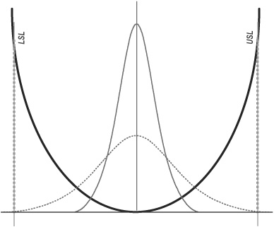
FIGURE 31-3. TAGUCHI LOSS FUNCTION

This is where statistical terminology comes into play. In Figure 31-2, the predictable process mean is centered between the specification limits, and there is a statistical distance of three standard deviations (three sigma) from the mean to the specification limits. Theoretically, approximately 99.73 percent of all the reports would be delivered within the six day limits, or about 2,700 per million. If you cut that variation in half (to create the taller curve in Figure 31-3), there would be a statistical distance of six sigma from the process center to either specification. Approximately 70 percent would be delivered within one day of the fifteenth, 99.73 percent would be delivered within three days of the fifteenth, and only about two reports per billion would be delivered outside of the six-day specification.

Motorola, embarking on a long-term initiative to improve its quality, used this “six sigma” capability as its goal for quality improvement. Because of the shifts in production processes, Motorola equated six sigma performance with what was considered a more realistic 3.4 parts per million defective rather than the theoretical maximum of two parts per billion. The company put together a phase-gated project life cycle called MAIC (Measure, Analyze, Improve, Control), and assembled a set of quality tools to use in each phase. Jack Welch of GE and Larry Bossidy of Allied Signal adopted the Six Sigma approach and popularized it in business literature. As a result, the Six Sigma approach became a very marketable approach to Continuous Improvement. GE, Allied Signal, and others added D (Define) to the beginning of the life cycle, for requirements setting and chartering.

Figure 31-4 depicts some of the activities and deliverables at each phase of the DMAIC life cycle. In the Define phase, the Black Belt, team and Champion build a business case for the project, identify the process scope and define a progress measure, and baseline the data for the progress measure. They agree on a goal and articulate an objective. These become the basis for a project charter. In Measure, the team develops and analyzes a detailed process map (flow chart). The Black Belt stratifies the baseline data to look for areas of interest. In Analyze, root cause analysis, hypothesis testing and model building help identify the leverage points that will create the desired change in performance. In Improve, the team generates solutions and sets up experiments (pilots) to test them. The study the results of the pilot, and put together a rollout plan to implement the total solution, full-scale. Finally, in Control, control plans are put in place to monitor the new process, hold the gains, measure financial or other benefits, and watch for further improvement opportunities.

SIX SIGMA AND PROJECT MANAGEMENT

So, what can Project Management bring to Six Sigma? What can Six Sigma (and other quality initiatives) bring to Project Management? While there are some differences in the bodies of knowledge, each discipline brings knowledge, skills, abilities and a number of tools to the table, and elements of each discipline would enhance the other.

In the PMO

FIGURE 31-4. DMAIC FLOW

At the organizational level, any project-focused or matrix organization trying to implement a Six Sigma program would be very well served by integrating Six Sigma projects into its existing Project Management Office (PMO). Six Sigma implementations often fail because the projects are scoped poorly, resources or data are not available, the solution is not implemented, or the projects are incorrectly assigned to Black Belts when the projects are a poor fit for DMAIC.³ A well-run PMO, with a strategic focus and leaders experienced in scoping and resources, would avoid some of these problems. It would also be beneficial from an organizational change perspective because Six Sigma—instead of being another add on or “flavor of the month”—would be seen as an addition to “the way we do business.” Skilled portfolio managers in the PMO could ensure that the DMAIC and DMADV life cycles were used to best advantage on applicable projects.

At the same time, some of the process management, statistical rigor, and decision-making tools from the Six Sigma, SPC and Lean approaches could help a PMO make more rational decisions regarding prioritization, resource allocation, logistics, and risk analysis. Understanding which aspects of certain projects are repeatable processes and applying ongoing tracking and optimization could greatly enhance a PMO’s accuracy in scheduling and budgeting, help avoid quality problems, and reduce tendencies toward “gold plating.” Stochastic modeling is a very powerful tool for maximizing the potential end value of a portfolio, thus providing an excellent way to manage risks and benefits and building the optimum strategic prioritization scheme for any set of proposed projects.

As a project-based approach, it would seem intuitive that the project team leaders (“Black Belts”) would have—or would at least be required to learn—project management tools and skills. This is seldom the case in practice, though. Engineers, office managers, line workers and others who get the training to become Six Sigma Black Belts usually only have PMP certification by serendipity.

When Using a CMM

For any organization trying to get beyond level two of the Capability Maturity Model,⁴ the knowledge gained through a concerted effort at quality improvement is vital. Level three requires standardized, managed and defined processes; many of the tools used in the Define and Measure phases are very useful for studying, streamlining, standardizing and measuring processes. What this may require is that Project Managers understand that some aspects of what they do are repeatable processes that can be defined using these techniques.

A level four process is quantitatively managed, “controlled using statistical and other quantitative techniques. Quantitative objectives for quality and process performance are established and used as criteria in managing the process. Quality and process performance is understood in statistical terms and is managed throughout the life of the process.”⁵ Any Project Manager in an organization trying to achieve level four in project management would need to understand and use SPC techniques (control charts, capability studies—used throughout the DMAIC model), which provide the basis for this type of quantitative management. Root cause analysis, hypothesis testing and other statistical tools from Measure and Analyze provide tools for managing the process, keeping it in control and improving it. In addition, the statistical knowledge required to use these approaches would greatly enhance the Project Manager’s understanding and skill in the area of risk analysis.

If your project management or PMO process is a key business driver and you want to take it to level five, quality approaches become an absolute necessity. A level five process is “an optimizing process … a quantitatively managed (capability level 4) process that is improved based on an understanding of the common causes of variation inherent in the process. The focus of an optimizing process is on continually improving the range of process performance through both incremental and innovative improvements … Reaching capability level 5 for a process area assumes that you have stabilized the selected subprocesses and that you want to reduce the common causes of variation in that process.”⁶ Control charts are the only set of statistical tools for understanding common and special cause; SPC, Lean and Six Sigma provide proven approaches for both incremental and breakthrough improvements.

In Project Management Training

One would think that Six Sigma Black Belts—who usually receive four to six weeks’ training in team facilitation, process management and improvement tools, and statistical analysis—would also be trained as project managers. This is not always true, however. Project management skills are usually left to chance in Six Sigma. Although Black Belts are supposed to manage projects, getting project management training is considered an extra. Reasons given for this vary: reluctance to pay for more training, assumptions that project management is a skill that is easily learned “on the job,” assumptions that the Black Belt candidates were “already skilled project managers … that’s why we selected them”; these top the list of the reasons given to the author.

Black Belts would gain greatly from learning formal PM skills and tools, and adopting the rigors of PM discipline. Six Sigma projects are plagued with the triple constraints, just as every other project is. Every Black Belt should be able to work up a rough overall WBS for each phase of a DMAIC project, and a detailed WBS for each phase at the beginning of that phase, even though the final deliverables for the project itself won’t be known until the Improve phase. They should be able to lay out a GANNT chart and a Pert or CPM diagram, and use those tools to monitor progress toward completion. They have an excellent risk-management tool, Failure Mode Effects Analysis, which can easily be adapted for project risk management. Additionally, Black Belts need to understand that resources are not free; the ability to understand resource loading and allocation would go a long way toward managing costs associated with Six Sigma projects.

Likewise, Project Managers would be well served by taking some Six Sigma and Lean training. The analysis and problem-solving knowledge, skills, and abilities they would gain through a Black Belt course would greatly enhance their abilities to forecast, to plan, to deal with emergent problems quickly, and to analyze and mitigate risk.

REFERENCES

¹ Wheeler, D. J., and Chambers, D. S. (1992). Understanding Statistical Process Control, 2nd Ed. Knoxville, TN: SPC Press, Inc.

² Ragland, B. (2004); Presentation at Northern Trust Worldwide Operations and Technology Senior Management Meeting.

³ Johnson, L. A. (2009). Falling short. Six Sigma Forum Magazine 8(3), 19–22.

⁴ CMMI Product Team (2009). CMMI for Services, Version 1.2. Pittsburgh: Carnegie Mellon University.

⁵ Ibid., p 24.

⁶ Ibid., pp 24–25.