3. Referring to Ranges
IN THIS CHAPTER
Shortcut for Referencing Ranges
Referencing Ranges in Other Sheets
Referencing a Range Relative to Another Range
Use the Cells Property to Select a Range
Use the Offset Property to Refer to a Range
Use the Resize Property to Change the Size of a Range
Use the Columns and Rows Properties to Specify a Range
Use the Union Method to Join Multiple Ranges
Use the Intersect Method to Create a New Range from Overlapping Ranges
Use the ISEMPTY Function to Check Whether the Cell Is Empty
Use the CurrentRegion Property to Select a Data Range
Use the Areas Collection to Return a Noncontiguous Range
A range can be a cell, row, column, or a grouping of any of these. The RANGE object is probably the most frequently used object in Excel VBA—after all, you are manipulating data on a sheet. Although a range can refer to any grouping of cells on a sheet, it can refer to only one sheet at a time. If you want to refer to ranges on multiple sheets, you must refer to each sheet separately.
This chapter shows you different ways of referring to ranges such as specifying a row or column. You also will learn how to manipulate cells based on the active cell and how to create a new range from overlapping ranges.
The Range Object
The following is the Excel object hierarchy:
Application > Workbook > Worksheet > Range
The Range object is a property of the Worksheet object. This means it requires that a sheet be active or it must reference a worksheet. Both of the following lines mean the same thing if Worksheets(1) is the active sheet:
Range("A1")
Worksheets(1).Range("A1")
There are several ways to refer to a Range object. Range("A1") is the most identifiable because that is how the macro recorder refers to it. However, each of the following is equivalent when referring to a range:
Range("D5")
[D5]
Range("B3").Range("C3")
Cells(5,4)
Range("A1").Offset(4,3)
Range("MyRange") 'assuming that D5 has a
Name 'of MyRange
Which format you use depends on your needs. Keep reading—it will all make sense soon!
Syntax to Specify a Range
The Range property has two acceptable syntaxes. To specify a rectangular range in the first syntax, specify the complete range reference just as you would in a formula in Excel:
Range("A1:B5").Select
In the alternative syntax, specify the upper-left corner and lower-right corner of the desired rectangular range. In this syntax, the equivalent statement might be this:
Range("A1", "B5").Select
For either corner, you can substitute a named range, the Cells property, or the ActiveCell property. The following line of code selects the rectangular range from A1 to the active cell:
Range("A1", ActiveCell).Select
The following statement selects from the active cell to five rows below the active cell and two columns to the right:
Range(ActiveCell, ActiveCell.Offset(5, 2)).Select
Named Ranges
You probably have already used named ranges on your worksheets and in formulas. You can also use them in VBA.
Use the following code to refer to the range "MyRange" in Sheet1:
Worksheets("Sheet1").Range("MyRange")
Notice that the name of the range is in quotes—unlike the use of named ranges in formulas on the sheet itself. If you forget to put the name in quotes, Excel thinks you are referring to a variable in the program. One exception is if you use the shortcut syntax discussed in the next section. In this case, quotes are not used.
Shortcut for Referencing Ranges
A shortcut is available when referencing ranges. The shortcut uses square brackets, as shown in Table 3.1.
Table 3.1. Shortcuts for Referencing Ranges

Referencing Ranges in Other Sheets
Switching between sheets by activating the needed sheet can dramatically slow down your code. To avoid this slowdown, you can refer to a sheet that is not active by first referencing the Worksheet object:
Worksheets("Sheet1").Range("A1")
This line of code references Sheet1 of the active workbook even if Sheet2 is the active sheet.
If you need to reference a range in another workbook, include the Workbook object, the Worksheet object, and then the Range object:
Workbooks("InvoiceData.xlsx").Worksheets("Sheet1").Range("A1")
Be careful if you use the Range property as an argument within another Range property. You must identify the range fully each time. For example, suppose that Sheet1 is your active sheet and you need to total data from Sheet2:
WorksheetFunction.Sum(Worksheets("Sheet2").Range(Range("A1"), Range("A7")))
This line does not work. Why not? Because Range(Range("A1"), Range("A7")) refers to an extra range at the beginning of the code line. Excel does not assume that you want to carry the Worksheet object reference over to the other Range objects. So what do you do? Well, you could write this:
WorksheetFunction.Sum(Worksheets("Sheet2").Range(Worksheets("Sheet2"). _
Range("A1"), Worksheets("Sheet2").Range("A7")))
But this is not only a long line of code, it is difficult to read! Thankfully, there is a simpler way, using With...End With:
With Worksheets("Sheet2")
WorksheetFunction.Sum(.Range(.Range("A1"), .Range("A7")))
End With
Notice now that there is a .Range in your code, but without the preceding object reference. That’s because With Worksheets("Sheet2") implies that the object of the range is the worksheet.
Referencing a Range Relative to Another Range
Typically, the RANGE object is a property of a worksheet. It is also possible to have RANGE be the property of another range. In this case, the Range property is relative to the original range, which makes for unintuitive code. Consider this example:
Range("B5").Range("C3").Select
This code actually selects cell D7. Think about cell C3, which is located two rows below and two columns to the right of cell A1. The preceding line of code starts at cell B5. If we assume that B5 is in the A1 position, VBA finds the cell that would be in the C3 position relative to B5. In other words, VBA finds the cell that is two rows below and two columns to the right of B5, which is D7.
Again, I consider this coding style to be very unintuitive. This line of code mentions two addresses, and the actual cell selected is neither of these addresses! It seems misleading when you are trying to read this code.
You might consider using this syntax to refer to a cell relative to the active cell. For example, the following line of code activates the cell three rows down and four columns to the right of the currently active cell:
Selection.Range("E4").Select
This syntax is mentioned only because the macro recorder uses it. Recall that when you recorded a macro in Chapter 1, “Unleash the Power of Excel with VBA,” with Relative References on, the following line was recorded:
ActiveCell.Offset(0, 4).Range("A2").Select
This line found the cell four columns to the right of the active cell, and from there it selected the cell that would correspond to A2. This is not the easiest way to write code, but that is the way the macro recorder does it.
Although a worksheet is usually the object of the Range property, occasionally, such as during recording, a range may be the property of a range.
Use the Cells Property to Select a Range
The Cells property refers to all the cells of the specified range object, which can be a worksheet or a range of cells. For example, this line selects all the cells of the active sheet:
Cells.Select
Using the Cells property with the Range object might seem redundant:
Range("A1:D5").Cells
This line refers to the original Range object. However, the Cells property has an Item property that makes the Cells property very useful. The Item property enables you to refer to a specific cell relative to the Range object.
The syntax for using the Item property with the Cells property is as follows:
Cells.Item(Row,Column)
You must use a numeric value for Row, but you may use the numeric value or string value for Column. Both of the following lines refer to cell C5:
Cells.Item(5,"C")
Cells.Item(5,3)
Because the Item property is the default property of the RANGE object, you can shorten these lines as follows:
Cells(5,"C")
Cells(5,3)
The ability to use numeric values for parameters is particularly useful if you need to loop through rows or columns. The macro recorder usually uses something like Range("A1").Select for a single cell and Range("A1:C5").Select for a range of cells. If you are learning to code only from the recorder, you might be tempted to write code like this:
FinalRow = Cells(Rows.Count, 1).End(xlUp).Row
For i = 1 to FinalRow
Range("A" & i & ":E" & i).Font.Bold = True
Next i
This little piece of code, which loops through rows and bolds the cells in Columns A through E, is awkward to read and write. But, how else can you do it?
FinalRow = Cells(Rows.Count, 1).End(xlUp).Row
For i = 1 to FinalRow
Cells(i,"A").Resize(,5).Font.Bold = True
Next i
Instead of trying to type the range address, the new code uses the Cells and Resize properties to find the required cell, based on the active cell.
Using the Cells Property in the Range Property
Cells properties can be used as parameters in the Range property. The following refers to the range A1:E5:
Range(Cells(1,1),Cells(5,5))
This is particularly useful when you need to specify your variables with a parameter, as in the previous looping example.
Use the Offset Property to Refer to a Range
You have already seen a reference to Offset when the macro recorder used it when you recorded a relative reference. Offset enables you to manipulate a cell based off the location of the active cell. In this way, you do not need to know the address of a cell.
The syntax for the Offset property is as follows:
Range.Offset(RowOffset, ColumnOffset)
The syntax to affect cell F5 from cell A1 is
Range("A1").Offset(RowOffset:=4, ColumnOffset:=5)
Or, shorter yet, write this:
Range("A1").Offset(4,5)
The count of the rows and columns starts at A1 but does not include A1.
But what if you need to go over only a row or a column, but not both? You don’t have to enter both the row and column parameter. If you need to refer to a cell one column over, use one of these lines:
Range("A1").Offset(ColumnOffset:=1)
Range("A1").Offset(,1)
Both lines mean the same, so the choice is yours. Referring to a cell one row up is similar:
Range("B2").Offset(RowOffset:=-1)
Range("B2").Offset(-1)
Once again, you can choose which one to use. It is a matter of readability of the code.
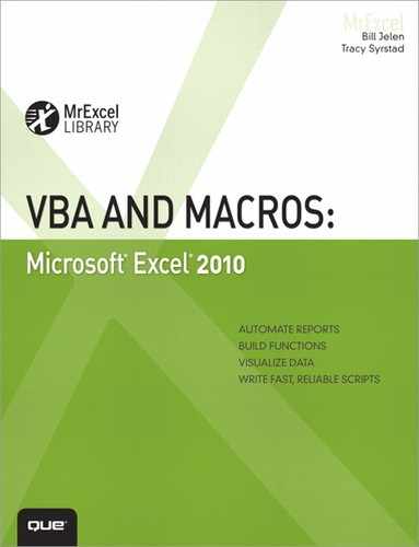
Suppose you have a list of produce with totals next to them. If you want to find any total equal to zero and place LOW in the cell next to it, do this:
The LOW totals are noted by the program, as shown in Figure 3.1.

Figure 3.1. Find the produce with zero totals.
Note
Refer to the section “Object Variables” in Chapter 5 for more information on the Set statement.
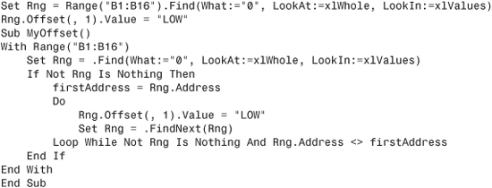
Offsetting isn’t only for single cells—it can be used with ranges. You can shift the focus of a range over in the same way you can shift the active cell. The following line refers to B2:D4 (see Figure 3.2):
Range("A1:C3").Offset(1,1)
Figure 3.2. Offsetting a range: Range("A1:C3").Offset(1,1).Select.
Use the Resize Property to Change the Size of a Range
The Resize property enables you to change the size of a range based on the location of the active cell. You can create a new range as needed. The syntax for the Resize property is
Range.Resize(RowSize, ColumnSize)
To create a range B3:D13, use the following:
Range("B3").Resize(RowSize:=11, ColumnSize:=3)
Or a simpler way to create this range:
Range("B3").Resize(11, 3)
But what if you need to resize by only a row or a column, not both? You do not have to enter both the row and column parameters.
If you need to expand by two columns, use one of the following:
Range("B3").Resize(ColumnSize:=2)
or
Range("B3").Resize(,2)
Both lines mean the same. The choice is yours. Resizing just the rows is similar. You can use either of the following:
Range("B3").Resize(RowSize:=2)
or
Range("B3").Resize(2)
Once again, the choice is yours. It is a matter of readability of the code.
From the list of produce, find the zero totals and color the cells of the total and corresponding produce (see Figure 3.3):
Set Rng = Range("B1:B16").Find(What:="0", LookAt:=xlWhole, LookIn:=xlValues)
Rng.Offset(, -1).Resize(, 2).Interior.ColorIndex = 15
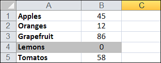
Figure 3.3. Resizing a range to extend the selection.
Notice that the Offset property was used first to move the active cell over. When you are resizing, the upper-left corner cell must remain the same.
Resizing isn’t only for single cells—it can be used to resize an existing range. For example, if you have a named range but need it and the column next to it, use this:
Range("Produce").Resize(,2)
Remember, the number you resize by is the total number of rows/columns you want to include.
Use the Columns and Rows Properties to Specify a Range
Columns and Rows refer to the columns and rows of a specified Range object, which can be a worksheet or a range of cells. They return a Range object referencing the rows or columns of the specified object.
You have seen the following line used, but what is it doing?
FinalRow = Cells(Rows.Count, 1).End(xlUp).Row
This line of code finds the last row in a sheet in which Column A has a value and places the row number of that Range object into FinalRow. This can be useful when you need to loop through a sheet row by row—you will know exactly how many rows you need to go through.
Caution
Some properties of columns and rows require contiguous rows and columns to work properly. For example, if you were to use the following line of code, 9 would be the answer because only the first range would be evaluated:
Range("A1:B9, C10:D19").Rows.Count
However, if the ranges are grouped separately the answer would be 19.
Range("A1:B9", "C10:D19").Rows.Count
Use the Union Method to Join Multiple Ranges
The Union method enables you to join two or more noncontiguous ranges. It creates a temporary object of the multiple ranges, which allows you to affect them together:
Application.Union(argument1, argument2, etc.)
The following code joins two named ranges on the sheet, inserts the =RAND() formula, and bolds them:
Set UnionRange = Union(Range("Range1"), Range("Range2"))
With UnionRange
.Formula = "=RAND()"
.Font.Bold = True
End With
Use the Intersect Method to Create a New Range from Overlapping Ranges
The Intersect method returns the cells that overlap between two or more ranges:
Application.Intersect(argument1, argument2, etc.)
The following code colors the overlapping cells of the two ranges.
Set IntersectRange = Intersect(Range("Range1"), Range("Range2"))
IntersectRange.Interior.ColorIndex = 6
Use the ISEMPTY Function to Check Whether a Cell Is Empty
The ISEMPTY function returns a Boolean value of whether a single cell is empty; True if empty, False if not. The cell must truly be empty. Even if it has a space that you cannot see, Excel does not consider the cell to be empty:
IsEmpty(Cell)
Figure 3.4 has several groups of data separated by a blank row. You want to make the separations a little more obvious.

Figure 3.4. Blank empty rows separating data.
The following code goes down the data in Column A. When it finds an empty cell, it colors in the first four cells for that row (see Figure 3.5):
LastRow = Cells(Rows.Count, 1).End(xlUp).Row
For i = 1 To LastRow
If IsEmpty(Cells(i, 1)) Then
Cells(i, 1).Resize(1, 4).Interior.ColorIndex = 1
End If
Next i
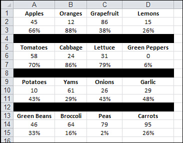
Figure 3.5. Colored rows separating data.
Use the CurrentRegion Property to Select a Data Range
CurrentRegion returns a Range object representing a set of contiguous data. As long as the data is surrounded by one empty row and one empty column, you can select the table with CurrentRegion:
RangeObject.CurrentRegion
The following line selects A1:D3 because this is the contiguous range of cells around cell A1 (see Figure 3.6):
Range("A1").CurrentRegion.Select
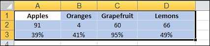
Figure 3.6. Use CurrentRegion to select a range of contiguous data around the active cell.
This is useful if you have a table whose size is in constant flux.
Case Study: Using the SpecialCells Method to Select Specific Cells
Even Excel power users may not have encountered the Go To Special dialog box. If you press the F5 key in an Excel worksheet, you get the normal Go To dialog box (see Figure 3.7). In the lower-left corner of this dialog is a button labeled Special. Click that button to get to the super-powerful Go To Special dialog (see Figure 3.8).
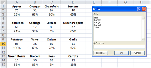
Figure 3.7. Although the Go To dialog doesn’t seem useful, click the Special button in the lower-left corner.

Figure 3.8. The Go To Special dialog has many incredibly useful selection tools.
In the Excel interface, the Go To Special dialog enables you to select only cells with formulas, only blank cells, or only the visible cells. Selecting only visible cells is excellent for grabbing the visible results of AutoFiltered data.
To simulate the Go To Special dialog in VBA, use the SpecialCells method. This enables you to act on cells that meet a certain criteria:
RangeObject.SpecialCells(Type, Value)
This method has two parameters: Type and Value. Type is one of the xlCellType constants:
xlCellTypeAllFormatConditions
xlCellTypeAllValidation
xlCellTypeBlanks
xlCellTypeComments
xlCellTypeConstants
xlCellTypeFormulas
xlCellTypeLastCell
xlCellTypeSameFormatConditions
xlCellTypeSameValidation
xlCellTypeVisible
Value is optional and can be one of the following:
xlErrors
xlLogical
xlNumbers
xlTextValues
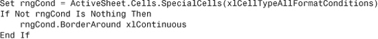
The following code returns all the ranges that have conditional formatting set up. It produces an error if there are no conditional formats and adds a border around each contiguous section it finds:
Have you ever had someone send you a worksheet without all the labels filled in? Some people consider that the data shown in Figure 3.9 looks neat. They enter the Region field only once for each region. This might look aesthetically pleasing, but it is impossible to sort. Even Excel’s pivot table routinely returns data in this annoying format.

Figure 3.9. The blank cells in the region column make it difficult to sort data tables such as this.
Using the SpecialCells method to select all the blanks in this range is one way to fill in all the blank region cells quickly with the region found above them:
In this code, Range("A1").CurrentRegion refers to the contiguous range of data in the report. The SpecialCells method returns just the blank cells in that range. Although you can read more about R1C1 style formulas in Chapter 6, “R1C1-Style Formulas,” this particular formula fills in all the blank cells with a formula that points to the cell above the blank cell. The second line of code is a fast way to simulate doing a Copy and then Paste Special Values. Figure 3.10 shows the results.

Figure 3.10. After the macro runs, the blank cells in the Region column have been filled in with data.
Use the Areas Collection to Return a Noncontiguous Range
The Areas collection is a collection of noncontiguous ranges within a selection. It consists of individual Range objects representing contiguous ranges of cells within the selection. If the selection contains only one area, the Areas collection contains a single Range object corresponding to that selection.
You might be tempted to loop through the sheet, copy a row, and paste it to another section. However, there is an easier way (see Figure 3.11):
Range("A:D").SpecialCells(xlCellTypeConstants, 1).Copy Range("I1")
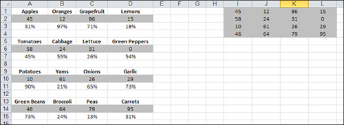
Figure 3.11. The Areas collection makes it easier to manipulate noncontiguous ranges.
Referencing Tables
With Excel 2007, you were introduced to a new way of interacting with ranges of data: tables. These special ranges offer the convenience of referencing named ranges, but they are not created in the same manner. For more information on how to create a named table, see Chapter 8, “Create and Manipulate Names in VBA.”
The table itself is referenced using the standard method of referring to a ranged name. To refer to the data in Table1 in Sheet1, do this:
Worksheets(1).Range("Table1")
This references the data part of the table but does not include the header or total row. To include the header and total row, do this:
Worksheets(1).Range("Table1[#All]")
What I really like about this feature is the ease of referencing specific columns of a table. You don’t have to know how many columns in from a starting position or the letter/number of the column, and you don’t have to use a FIND function. Instead, you can use the header name of the column. For example, do this to reference the Qty column of the table:
Worksheets(1).Range("Table1[Qty]")
Next Steps
Now that you have an idea of how Excel works, it’s time to apply it to useful situations. Chapter 4, “User-Defined Functions,” uses the skills you have learned so far and introduces other programming methods that you will learn more about throughout this book.