Who’s Ahead?
20.1 THE PROBLEM
Suppose two candidates for office, P and Q, receive p and q votes, respectively, where p > q. That is, P wins. That final result is definitively established, however, only after the ballot-counting process is completed. During the counting process the lead can switch back and forth, depending on the particular order in which the individual ballots are processed. A famous result in nineteenth-century probability theory called the ballot theorem says that the probability P is always ahead of Q from the first counted ballot is given by
![]()
This simple expression has a rather surprising implication. Suppose, for example, that P wins by a 4-to-1 margin (a huge victory), with p = 400 and q = 100. Then the ballot theorem says P is always ahead of Q in the count with probability
![]()
which says that, even with P’s huge victory, the probability is a not insignificant 0.4 that sometime during the counting process Q will be in at least a tie with P.
The ballot theorem was first proved by the English mathematician William Allen Whitworth (1840–1905) in 1878, although many modern writers still (mistakenly) attribute it to the French mathematician Joseph Bertrand (1822–1900), who indeed also derived the result, but not until nearly a decade later, in 1887. The result is so simple in appearance that it seems as though it should have an equally simple derivation. It does, but it’s simple only in the math required. What makes the math simple is an extremely clever geometrical observation. Before I show it to you, try your own hand at proving the ballot theorem. You’ll then better appreciate the trick!
20.2 THEORETICAL ANALYSIS
As the ballots are taken from the voting box to be counted, we can plot the results as shown in Figure 20.2.1, where the horizontal axis is the number of ballots processed so far and the vertical axis is the current net total count for P. That is, the positive vertical axis means P is ahead (Q is behind), the negative vertical axis means P is behind (Q is ahead), and the horizontal axis itself represents a tie. The plot (called a path) shown in Figure 20.2.1 is for the particular vote-counting sequence that starts with p p p q p q q p q q. … We’ll call any path that has this particular start (no matter what happens thereafter as additional votes are counted) a bad path since they all are paths in which P is not always ahead of Q (because we have a tie after the tenth vote is counted). A good path would be any path that is always above the horizontal axis after the first vote is counted. Path geometry seems simple enough, but it is powerful enough to be the key to solving our problem.
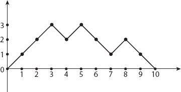
Figure 20.2.1. A bad counting path.
With our observation in mind, we can now conclude that all paths that begin with a vote for Q are bad paths, since they immediately fall below the horizontal axis. The probability of the first counted ballot being for Q is
![]()
Next, consider the case where P wins the election with the final count of 4 to 3. Figure 20.2.2 shows the path for the particular counting sequence p p q q q p p. This path starts off looking like a good path, but eventually it “goes bad” after the fourth ballot because, at that point, there is a tie.
Since there is a tie, then at that point we know (by definition!) there have been an equal number of votes for P and Q. This isn’t as trivial as it may sound, because it means that it is possible to rearrange the counting sequence from starting as p p q q to q q p p; that is, up to the first tie, replace each p with a q and each q with a p, as shown in Figure 20.2.3. The resulting new path is called a reflected path (up to the first tie). It is always possible to do this with a “good path gone wrong” because of the equal number of votes for P and for Q up to the first tie. Doing this has turned the good path gone wrong into a path “bad from the start,” that is, into a path that we have already considered in the previous discussion.
The reverse reflection is also possible, too, and that means there is a one-to-one correspondence between good paths gone wrong and paths

Figure 20.2.2. Another bad counting path.

Figure 20.2.3. The reflection of the path in Figure 20.2.2.
bad from the start. That is, they have the same probability. So, the total probability of bad paths is just
![]()
All other paths are good paths, and so the probability of good paths, paths for which P is always ahead of Q, is
![]()
and, just like that, we have the ballot theorem.