
To Test—Or Not to Test?
17.1 THE PROBLEM
In our modern times, new and wonderful advances are seemingly achieved between the last time we turned the TV off and when we turn it back on. This is particularly true in medicine, where apparently there is a treatment for every ill that afflicts the human body, ranging over the entire spectrum from warts and dry eyes to erectile dysfunction and urinary incontinence to asthma and bowel disease to. … Well, you get the idea, and the message, too: drug companies have spent billions of dollars telling us to “ask your doctor” about the latest pills, patches, injections, inhalers, and drops to arrive at the local drugstore.
We are also told to have regular diagnostic tests for all sorts of awful things, from mammograms for women (breast cancer) to blood PSA levels for men (prostate cancer) to colonoscopies, blood sugar levels, abdominal ultrasounds, and chest X-rays for everybody (to detect colon cancer, diabetes, aortic aneurysm, and lung cancer, respectively). While any of those tests is almost surely “good for you,” such testing does come with a potentially serious issue. It is, alas, simply not perfect. That is, any diagnostic test has associated with it two quite different statistical errors, the false positive and the false negative.
A false positive occurs when a test says you have the condition tested for when you actually don’t. The usual result in that case is that you are scared silly (at least at first) and then later (more extensive and usually more expensive) testing reveals you are really okay. A false negative occurs when a test says you don’t have the condition tested for when you actually do. This is potentially a far more serious outcome than is a false positive result because it can lull you into a sense of security and encourage you to take no further action—and then, a month or so later, perhaps, you suddenly drop dead. That’s particularly sad when you think that a ten-cent-a-day pill might have given you another fifty years!
With these scary considerations in mind, you can understand why it is an important goal in any medical trial of a new diagnostic test to determine the statistical behavior of the test. For example, let’s suppose you have decided to take a newly developed test for a terrible condition, one whose very name is unspeakable in other than a hushed whisper: awfulitis. It is estimated that only one in ten thousand people have awfulitis, but since it either kills you with probability 0.99 or, with probability 0.01, makes you wish it had killed you, you are plenty worried about it. Now, clearly, either you have awfulitis or you don’t, which we’ll denote by A and ![]() , respectively. When you take the test it will, equally clearly, say either you have awfulitis or that you don’t, which we’ll denote by T and
, respectively. When you take the test it will, equally clearly, say either you have awfulitis or that you don’t, which we’ll denote by T and ![]() , respectively.
, respectively.
The probability of a false positive when you take the test, in the notation of conditional probability, is written as P(T | ![]() ), which is read as “the probability the test says you have awfulitis given that you actually don’t.” (The “given” part is always to the right of the vertical bar.) The probability of a false negative when you take the test is written as P(
), which is read as “the probability the test says you have awfulitis given that you actually don’t.” (The “given” part is always to the right of the vertical bar.) The probability of a false negative when you take the test is written as P(![]() | A), which is read as “the probability the test says you don’t have awfulitis given that you actually do.”
| A), which is read as “the probability the test says you don’t have awfulitis given that you actually do.”
Extensive trials, using groups of people known either to have or not to have awfulitis, have determined that
P(T | A) = 0.95
and
P(![]() |
| ![]() ) = 0.95.
) = 0.95.
These two results contain within them the probabilities of both the false negative and false positive errors, because we can write
P(T | A) + P(![]() | A) = 1
| A) = 1
and
In each of these two equations we hold the given part fixed, and then add the conditional probabilities of each of the two possible test outcomes. The sum in each case must be 1, because “given a fixed condition,” the test will say something. So, we have
P(![]() | A) = 1 − P(T | A) = 0.05 (probability of false negative)
| A) = 1 − P(T | A) = 0.05 (probability of false negative)
and
P(T | ![]() ) = 1 − P(
) = 1 − P(![]() |
| ![]() ) = 0.05 (probability of false positive).
) = 0.05 (probability of false positive).
To most people, these seem like pretty impressive numbers. Zero probability for both kinds of errors would be best, of course, but 0.05 looks small. But is 0.05 small enough? The way to answer that question is to ask yourself what you would do after being told the test result. Suppose you are told that the test says you have awfulitis. But do you? Or suppose the test says you don’t have awfulitis. Is that true? In the first case, what you’d want to calculate is P(A | T), the conditional probability that you have awfulitis given that the test says you do. And in the second case, you’d want to calculate P(![]() |
| ![]() ), or the conditional probability that you don’t have awfulitis given that the test says you don’t. My personal experience is that many family doctors often do not know how to do these calculations, or even that such calculations can be done. So, what are these conditional probabilities for awfulitis?
), or the conditional probability that you don’t have awfulitis given that the test says you don’t. My personal experience is that many family doctors often do not know how to do these calculations, or even that such calculations can be done. So, what are these conditional probabilities for awfulitis?
17.2 THEORETICAL ANALYSIS
From conditional probability theory we have the fundamental definition
![]()
Like most definitions in mathematics this has not simply been pulled out of the air but rather is motivated by a specific, special case. Imagine a finite sample space with N different, equally likely sample points. Of these N points, nA are associated with A, nT are associated with T, and nAT are common to both A and T. Then
![]()
from which we immediately have our definition. In exactly the same way we have
![]()
which says
P(AT) = P(T | A) P(A),
and so
![]()
The theorem of total probability says1
P(T) = P(T | A) P(A) + P(T | ![]() ) P(
) P(![]() ),
),
and so
![]()
We know all of the probabilities on the right (one person in 10,000 having awfulitis means P(A) = 0.0001 and so P(![]() ) = 0.9999):
) = 0.9999):

a result that, without fail, astonishes everybody. The test is almost surely wrong if it says you have awfulitis!
This is an important calculation to perform because in addition to making you feel better—Thank God, I’m (almost surely) not going to die!—the calculation tells researchers what has to change to improve the test. P(A | T) is small because of the large term in the denominator due to P(T | ![]() ) P(
) P(![]() ). There’s nothing we can do about the P(
). There’s nothing we can do about the P(![]() ) factor; even if you could do something about it, there isn’t much left to do, as it’s practically 1 already and, if it were 1 (which means nobody has awfulitis), that would eliminate the need in the first place for the test. Rather, it’s the factor P(T |
) factor; even if you could do something about it, there isn’t much left to do, as it’s practically 1 already and, if it were 1 (which means nobody has awfulitis), that would eliminate the need in the first place for the test. Rather, it’s the factor P(T | ![]() ) = 1 − P(
) = 1 − P(![]() |
| ![]() ) that needs to be greatly reduced. In other words, P(
) that needs to be greatly reduced. In other words, P(![]() |
| ![]() ) = 0.95, which initially looked so good, actually isn’t nearly good enough, and must be increased. Suppose, for example, that we could make P(
) = 0.95, which initially looked so good, actually isn’t nearly good enough, and must be increased. Suppose, for example, that we could make P(![]() |
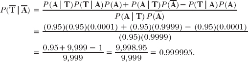
| ![]() ) = 0.9999. That sure looks good! Well, let’s see if it is.
) = 0.9999. That sure looks good! Well, let’s see if it is.
This new value for P(![]() |
| ![]() ) gives P(T |
) gives P(T | ![]() ) = 0.0001, and so
) = 0.0001, and so

which is a big improvement, but the test is still wrong more often than it’s right.
Okay, let’s stop guessing and approach this in reverse. What must P(![]() |
| ![]() ) be so that P(A | T) = 0.95? We have
) be so that P(A | T) = 0.95? We have
![]()
and so, solving for P(![]() |
| ![]() ) gives
) gives
That is, given a million people who are known not to have awfulitis, the test must say (erroneously) that, at most, five of them have awfulitis.
For our last calculation, that of P(![]() |
| ![]() ), doing the same sort of analysis as we did for P(A | T) should allow you to derive
), doing the same sort of analysis as we did for P(A | T) should allow you to derive

That is, as it stands the test is a very good test if it declares you to be free of awfulitis. So, the bottom line concerning our diagnostic test is: if the news is bad, then certainly do a follow-up test (and you’re probably okay anyway), while if the news is good, you (almost certainly) are okay.
Historical Note
This sort of probabilistic analysis (called Bayesian analysis, after the English minister Thomas Bayes [1701–1761], who initiated such calculations in a posthumously published 1764 paper in the Philosophical Transactions of the Royal Society of London) has been unfairly burdened over the years with some unfortunate applications. The best known of these misuses is probably Laplace’s infamous calculation of the probability the sun will rise tomorrow.
Beginning in 1744, the French mathematician Pierre-Simon Laplace (1749–1827) began writing on what is known as his “law of succession,” which answers the following question: if an event in a repeatable probabilistic experiment has been observed to happen n times in a row, what is the probability that event will happen yet again in the very next experiment? The experiment might be the flipping of a coin or, in Laplace’s erroneous example, the rising of the sun. Laplace’s starting point in his analysis was with the assumption of total ignorance, which, in the coin-flipping example, means all possible values for the probability of heads are equally likely (uniform from 0 to 1). Since this analysis has historical value, let me now show you a balls-and-urns derivation of Laplace’s result.
Suppose you are confronted with N + 1 urns, each of which contains N balls. The urns are numbered from 0 to N, with urn k containing k black balls and N − k white balls (urn 0 has all white balls and urn N has all black balls). Now, imagine that you select an urn at random and then make n consecutive drawings from it, each time replacing the ball after observing its color. If all n of those drawings resulted in a black ball, then what’s the probability the next drawing will also result in a black ball? This is obviously a conditional probability, in that if A is the event “n drawings of n black balls” and B is the event “next drawing will be a black ball,” then what we are asking for is P(B | A). The fact that we first select (at random) one urn from urns representing all possible combinations of black and white balls is the way this problem models Laplace’s assumption of total ignorance.
Given that we first select urn k, then the probability of drawing a black ball n straight times (event A) is
![]()
where Uk is the event “urn k selected.” From the theorem of total probability we can write
![]()
and, since P(Uk) = 1/(N + 1), we have
![]()
AB is the joint event of “n drawings of n black balls and the next (that is, the n + 1st drawing) is also a black ball,” which means n + 1 drawings have produced n + 1 black balls. From our last result, for P(A), we have P(AB) given by just replacing n with n + 1 to get
![]()
Also, note that P(AB) = P(B) since if we have had n + 1 consecutive black balls drawn (event B), then event A (n consecutive black balls drawn) has also occurred.
Thus, the (conditional) probability of interest, P(B | A), is
The sum in the denominator in this expression can be approximated by the integral of xn as x varies from 0 to N, and we can do the same for the numerator. Thus,

As a colorful illustration of this result, Laplace replaced the successive drawings of black balls out of an urn with the successive risings of the sun. In his 1814 A Philosophical Essay on Probabilities he wrote, “Placing the most ancient epoch of history at five thousand years ago, or at 1,826,213 days, and the sun having risen constantly in the interval at each revolution of twenty-four hours, it is a bet of 1826214 to one that it will rise again tomorrow.” Analysts have ever since ridiculed Laplace’s words as nonsense, as describing a situation that violates the very ideas of a “repeatable probabilistic experiment.” There is nothing at all random about the sun rising, with Newton’s inverse-square law of gravity and celestial mechanics being behind that daily event.
Was Laplace serious with his example? He was, after all, a genius. In fact, Laplace knew perfectly well the example was flawed, as the very next sentence (one usually not quoted by his critics) after the one quoted above is, “But this number is comparably greater for him who, recognizing in the totality of phenomena the principal regulator of days and seasons [my emphasis], sees that nothing at the present moment can arrest the course of it [the rising of the sun].” Laplace, in looking for a dramatic illustration for his law of succession, simply went a step too far, with the unfortunate consequence of throwing a shadow over Bayesian analysis in general. The use we made of it in the medical test analysis earlier in this chapter is perfectly fine.
1. This result should be self-evident by writing the right-hand side as
![]()
which is the probability T occurs and A does, too, plus the probability T occurs and A doesn’t. That is, the sum is simply the probability T occurs, and we don’t care whether A does or doesn’t. But that is precisely P(T).