16

Big Quotients—Part 2

16.1 THE PROBLEM

A quick recap from the end of Problem 5: we pick N numbers uniformly from 0 to 1, divide the largest by the smallest, and ask for the probability that the result is larger than k, for any k ≥ 1. This is a significantly more difficult question to answer than was the original Problem 5 question, where we treated in detail the special case of N = 2. We could, in theory, proceed just as before, looking now at an N-dimensional unit cube and the subvolumes in that cube that correspond to our problem (in Problem 5 the “cube” was a two-dimensional square and the subvolumes were the shaded triangles in Figure 5.2.1). It’s pretty hard to visualize in the Nth dimension, however, so here I’ll instead take a purely analytical approach. This will prove to be one of the longer analyses in this book, but I think you’ll find it to be a most impressive illustration of the power of mathematics.

16.2 THEORETICAL ANALYSIS

What we wish to calculate is

where the index i runs from 1 to N and the X_i are independent, uniformly distributed random numbers from 0 to 1. We can reduce this back down to a two-dimensional problem by defining the random variables U = min{X_i} and V = max {X_i} and asking for

Figure 16.2.1. The probability of the shaded area is Prob(V > kU).

This reduction will come at a price, as you’ll soon see. But it will be a price we can pay with just undergraduate mathematics!

In Figure 16.2.1 I’ve again drawn a two-axis coordinate system, similar to Figure 5.2.1, with V on the vertical axis and U on the horizontal axis. Clearly, both U and V take their values from the interval 0 to 1. The shaded area represents that portion of the unit square (in the first quadrant) where V ≥ kU, but now the probability associated with that area is not the area itself (as it was in Problem 5). That’s because neither V nor U is uniformly distributed from 0 to 1, and this is a most important point. To demonstrate the nonuniformity of both V and U is not difficult, and it will be useful to go through such a demonstration as it involves arguments we’ll use later in this analysis.

We start by considering the distribution function of V, defined as

F_V (v) = Prob(V ≤ v) = Prob(max {X_i} ≤ v).

Now, if the largest X_i ≤ v, then certainly all of the other X_i ≤ v, too, and so

F_V (v) = Prob(X₁ ≤ v, X₂ ≤ v, …, X_N ≤ v),

and so, since the X_i are independent, we then have

F_V (v) = Prob(X₁ ≤ v) Prob(X₂ ≤ v) … Prob(X_N ≤ v).

That is, the distribution function for V is the product of the distribution functions for each of the individual X_i. All of the X_i have the same distribution function because each X_i is identically distributed (uniformly random from 0 to 1). Therefore, if we write the distribution function for each X_i as

Prob(X ≤ v) = F_X(v),

then

Okay, but what is F_X(v)? Since X is uniform from 0 to 1, then

Prob(X ≤ v) = Prob(0 ≤ X ≤ v) = v,

a linear function. Thus, random variables that are uniform have linear distributions. But we have just shown that

F_V(v) = v^N,

which is not linear in v. Thus, the random variable V = max{X_i} is not uniformly distributed.

We have to do a slightly more sophisticated analysis to show that U = min{X_i} isn’t uniform, either. We start by writing the distribution function of U as

F_U(u)= Prob(U ≤ u)= Prob(min{X_i} ≤ u).

We have to come up with a new trick now because, unlike what we did in our first argument with the max function, we cannot argue that if the minimum of the X_i ≤ u, then all the X_i ≤ u. But what we can write is

Prob{min{X_i} > u} = Prob{all of the X_i > u} = Prob(X₁ > u) … Prob(X_N > u)

since if the smallest X_i > u, then all the other X_i are at least as large. Now,

Prob{min{X_i} > u} = 1 − Prob(min{X_i} ≤ u) = 1 − F_U(u),

and so

1 − F_U(u) = [1 − Prob(X₁ ≤ u)] [1 − Prob(X₂ ≤ u)] … [1 − Prob(X_N ≤ u)],

or

1 − F_U(u) = [1 − F_X1(u)] [1 − F_X2(u)] … [1 − F_XN(u)],

or, again because each of the X_i has the same distribution function,

F_U(u) = 1 − [1 − F_X(u)]^N.

Since F_X(u) = u, then the distribution of U is

F_U(u) = 1 − [1 − u]^N,

which is definitely not linear in u. Thus, the random variable U = min{X_i} is not uniformly distributed. This means, as I said before, that we cannot equate the value of the area of the shaded region in Figure 16.2.1 to the value of the probability of the event V > kU. What we need to do to calculate that probability is a bit more sophisticated.

The probability density function of V, written as f_V (v), is a function such that

where z is simply a dummy variable of integration. That is, the distribution is the integral of the density. In the same way, the probability density function of U is f_U(u), where

If we differentiate both sides of these two equations, we have

and

That is, the density of a random variable is the derivative of the distribution.

The densities for the maximum and the minimum functions, in the general case of identically distributed X_i with arbitrary density (not necessarily restricted to being uniform from 0 to 1), are

and

f_U(u) = N[1 − F_X(u)]^{N − 1} f_X(u).

We’ll use the distribution and density functions for both U and V again later in this book (Problem 19), and so these calculations will have a further payoff for us when we are done with our present problem.

When we have a problem involving two random variables, as we do here, we can define what is called the joint probability density, written as f_{U, V} (u, v)—recall our analysis in Problem 14. Just as integrating the density over an interval gives us the probability a random variable has a value from that interval, integrating a joint density over a region gives us the probability our two random variables have values that locate a point in that region—again, recall Problem 14. So, the probability we are after, Prob(V > kU), is the integral of the joint density of U and V over the shaded region of Figure 16.2.1. That is,

where the inner u-integration is along a horizontal strip (distance v up from the U axis), and the outer v-integration moves the horizontal strip upward, starting from v = 0 and ending at v = 1. That is, our double integral vertically scans the shaded region. What we need to do next, then, is find the joint density of U and V so that we can perform the integrations.

If U and V were independent, then the joint density would simply be the product of the individual densities—you’ll recall this is what we were able to do in Problem 14. Our U and V in this problem, however, are not independent. After all, if I tell you what U is, then you immediately know V is bigger. Or if I tell you what V is, then you immediately know U is smaller. That is, knowledge of either U or of V gives you knowledge of the other, and so

f_{U, V}(u, v) ≠ f_U(u) f_V(v).

Okay, this is what we can’t do; what can we do?

Generalizing to two random variables considered together, we can define their joint distribution function F_{U, V}(u, v) as

and so extending the idea of getting a density by differentiating a distribution, the joint density f_{U, V}(u, v) is given by a double differentiation:

What we need to do, then, is find the joint distribution of U and V, then partially differentiate it twice to get the joint density, and then integrate that density over the shaded region in Figure 16.2.1. This sounds like a lot to do, but in fact, it really isn’t that hard, as I’ll now show you.

To find F_{U, V} (u, v), there are two cases to consider, that of u ≥ v and u < v. For the first case, the upper bound u on the minimum X_i is greater than the upper bound on the maximum X_i, and so of course the value of u really plays no role; after all, if the maximum X_i can be no larger than v, then we know that all the X_i ≤ v, and so

Since there is no u dependency in F_{U, V}(u, v) for u ≥ v, then

f_{U, V}(u, v) = 0, u ≥ v.

For the second case, where u < v, the upper bound on the minimum is less than the upper bound on the maximum. All of the X_i ≤ v, of course, but now at least one of the X_i ≤ u, too. What this means is that all of the X_i cannot be in the interval u to v. That is, for u < v,

F_{U, V}(u, v) = Prob(all the X_i ≤ v) − Prob(all the X_i both > u and ≤ v).

The first probability on the right is

while the second probability on the right is

Prob(all the X_i both > u and ≤ v) = Prob(u < X₁ ≤ v) … Prob(u < X_N ≤ v)

= [F_X (v) − F_X (u)]^N.

Thus,

Differentiating first with respect to v, we have

and then differentiating again with respect to u,

which we see, as claimed earlier, is NOT

Since all the X_i in our problem are uniform from 0 to 1, we have

If you look back at Figure 16.2.1 you’ll see that over the entire shaded region of integration we have u < v, and so using the above expressions for the distributions and densities involved,

f_{U, V}(u, v) = N(N − 1) (v − u)^{N − 2}.

Thus, the formal answer to our question is the probability integral

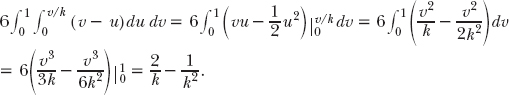
Notice that if N = 2 (the problem we solved by geometric means back in Problem 5) this integral reduces to

just as we found before.

16.3 COMPUTER SIMULATION

For N = 3, the case we could only simulate (with the code ratio2.m) at the end of Problem 5, our probability integral becomes

If you plug in the values of k that I used in Table 5.3.2 for the N = 3 case, you’ll find there is remarkably good agreement between the simulation results from ratio2.m and this theoretical result.

You should now be able to evaluate our probability integral for the N = 4 case, as well as modify ratio2.m to simulate the N = 4 case, and so again compare theory with experiment. Try it! If you feel really ambitious, do the integral in general—it actually isn’t that difficult—and show that

With this result, we can now answer the following question: how many numbers (all independently and randomly selected uniformly from 0 to 1) must be taken so that, with probability P, the ratio of the largest to the smallest is greater than k? We have

or

and so, taking logs on both sides and solving for N, we have

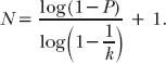
For example, if k = 4 and P = 0.9, then

and so N = 10.