
VALUATION
INTRODUCTION
If you are willing to accept the idea that financial markets are efficient, the next question becomes one of how investors price common stocks. What do they consider important? What do they consider irrelevant? And how do they decide what is the required rate of return for their money?
VALUING COMMON STOCK
The basic stock price valuation model is a discounted cash flow model in which the stock price is modeled as the present (discounted) value of the cash flows the investor expects to receive from owning the share. The model is often called the dividend valuation model because it can be represented mathematically as
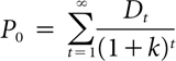
where
P0 = the price per share today
Dt = the expected per share cash dividend at the end of year t
k = the investors’ risk-adjusted required rate of return on the stock
And, if per share cash dividends are expected to grow by a constant annual percentage rate g forever and ever, the model reduces to

The discount rate used is the investors’ risk-adjusted required rate of return k, which is the return an investor can earn on other financial assets of identical risk. The manager should think of this required rate of return as the risk-adjusted return that the company must earn on investments in real assets.
For example, suppose the expected per share cash dividend for Ford Motor Company next year, D1, is $1.30; the investors’ required rate of return k on Ford’s common stock is 9.00 percent; and investors expect the annual growth rate g for Ford’s per share cash dividends to be 5.00 percent. With these expectations, we would estimate Ford’s stock price today to be $32.50 a share. The actual stock price may be more or less than $32.50, in which case, if you believe that markets are efficient, you have erred in estimating the dividend, the required rate of return, or the expected dividend growth rate.
As you can observe from the model, increases (decreases) in expected cash dividends and dividend growth rates cause an increase (decrease) in the stock price, as does a decrease (increase) in the investors’ required rate of return. Now we know how Ford managers can increase shareholder wealth: They can adopt policies that, other things being equal, lead to increases in cash dividends (either today or in the distant future) and/or lower the investors’ required rate of return. Let’s start with cash dividends.
Cash Dividends and Earnings
Cash dividends are paid out of earnings generated by investments in physical and human capital—let’s call it tangible and intangible capital. The higher the earnings, the higher the potential cash dividends. Thus, managers can increase shareholder wealth by making investments (in products, technologies, and so on) that generate high earnings, either today or in the future. Of course, these investments themselves require cash, so managers frequently have to choose between distributing the company’s earnings today as dividends or reinvesting them in the company to generate even higher earnings and cash flows in the future. It is this reinvestment of earnings in high-return projects today that produces an increase in g, the expected annual growth rate in cash dividends.
Investors’ Required Rate of Return
Knowledge about what determines the investors’ required rate of return is critical for managers who want to maximize the company’s stock price and for managers whose performance evaluation and compensation are tied to the market value of the company. So, let’s begin by breaking the investors’ required rate of return into two components: the risk-free nominal interest rate (RF) and a risk premium (RP). The risk-free nominal interest rate is the interest rate on default-free U.S. government bonds. Managers have no control over this rate; it is the same for every company. The risk premium depends on the riskiness of the firm’s after-tax cash flows to shareholders. Managers have varying degrees of control over this component.
Although most financial economists and practitioners believe that investors require higher rates of return as the riskiness of the investment increases, disagreement exists about just what risks investors are concerned about and how these risks are incorporated into stock prices. Basically, the issue boils down to whether investors factor into the price the total risk of a stock or only that portion of the risk that cannot be eliminated by holding the stock as part of a diversified investment portfolio.
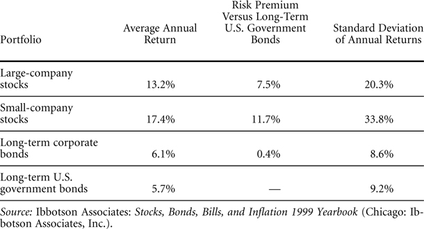
Figure 4-1 contains information about the historical returns that investors have earned on a variety of common stock portfolios and the riskiness of these portfolios. Since 1926, the yearly return that investors have earned on a portfolio of large-company stocks (such as the Fortune 500 companies) has averaged 13.2 percent. The yearly average for a portfolio of small-company stocks has been 17.4 percent. The average default-risk-free nominal rate of return on long-term U.S. government bonds has been 5.7 percent. So, at least in the United States, investors were able to earn considerably more on common stock investments than on risk-free bonds. However, the returns on common stocks were also considerably more risky. Risk, as measured by the yearly standard deviation of annual returns, was 33.2 percent for the small-stock portfolio, 20.3 percent for the large-company portfolio, and 5.7 percent for the default-free government bonds. In other words, for investors to reach for the higher average returns on small stocks, they had to accept a much greater variation in year-to-year returns than on government bonds.
FIGURE 4-1 AVERAGE ANNUAL RETURNS, RISK PREMIUMS, AND STANDARD DEVIATION OF RETURNS FOR SELECTED SECURITY PORTFOLIOS, 1926–1998
If we look at the standard deviation of the typical single stock and not a portfolio of stocks, however, it is around 50 percent even though the average expected return is the same as the portfolio return. Why? Well, the answer is that much of the risk associated with a single stock can be eliminated through diversification—holding the stocks of many different companies. The risk that can be eliminated through diversification is called unique risk and includes such risks as the success of the company’s advertising programs, new product developments, and changes in the company’s competitive position within its industry. The risk that cannot be eliminated is called market risk. Market risk refers to the effects that events that affect all companies in a country, such as interest-rate changes, recessions, and economic expansions, have on the financial fortunes of the company.
So, which risk should managers focus on when they evaluate the likely outcome of specific investment and financing decisions on the company’s stock price? Total risk or market risk?
THE CAPITAL ASSET PRICING MODEL
A commonly used asset pricing model called the capital asset pricing model (CAPM) says that managers should use only the market risk because investors can eliminate the unique risk. This market risk is captured by a statistic called beta that measures how a company’s stock price moves relative to the market as a whole, as measured by, say, the Standard & Poor’s 500 index—the market average. A beta of 1.0 means that when the Standard & Poor’s 500 goes up (down) by 2 percent, the stock is also expected to go up (down) by 2 percent. Any change in the stock price of more or less than this 2 percent is due to factors unique to the company and will be offset by unrelated moves in other stocks in the investor’s portfolio. Stocks with betas greater than 1.0 are more risky than the average stock; stocks with betas less than 1.0 are less risky.
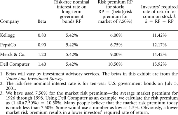
Figure 4-2 contains betas for several U.S. companies. Here is how a manager would use them to estimate what investors require in the way of a return on the equity capital they have committed to the company.
The manager first finds the yield on long-term government bonds from a financial newspaper or Web page. On July 5, 2001, it was 5.42 percent. This is the nominal risk-free interest rate RF. Next, the manager estimates what the risk premium should be for a well-diversified portfolio of common stocks. The risk premium, called the market risk premium, is the return the investor demands in excess of RF. Where does the manager get this number? Well, most managers begin by using the historical difference between the return on a portfolio of large-company stocks (13.2 percent in Figure 4-1) and the average return on long-term government bonds (5.7 percent). This calculation gives a market risk premium of 7.5 percent. Then the manager multiplies the risk premium on the market portfolio by the beta of the company. Let’s say the company is Kellogg. Kellogg’s beta is 0.80, so Kellogg’s required rate of return on its common stock on July 5, 2001, was 5.42% + 0.80(7.50%) = 11.42%. The required rates of return for the common stocks of the other companies are also listed in Figure 4-2.
FIGURE 4-2 BETAS AND INVESTORS’ REQUIRED RATES OF RETURN FOR THE COMMON STOCK OF SELECTED COMPANIES JULY 5, 2001
What does it mean to say that Kellogg’s required rate of return on its common stock is 11.42 percent? It means that Kellogg’s managers must earn this return on the investors’ equity investment in Kellogg in order to satisfy the investors. If managers fail to earn this return, individual and institutional investors will begin to ask why, and the managers may find themselves replaced and/or their companies restructured.
The major question confronting managers who need to evaluate how the riskiness of a project will affect the company’s stock price and future expected cash flows is what to do about unique risk. A company can fail because of unique risk events as well as because of systemic events. For example, investments in research and product development may not pay off, leaving the company in financial distress and the managers and employees without jobs. Yet it may be precisely these investments that are most likely to generate substantial increases in the stock price should they turn out successful new products. Now, the governance question becomes how to get managers and entrepreneurs to make such investments. These problems may well be among the most interesting governance problems for any governance system. We return to them repeatedly throughout the book.
DOES THE CAPM WORK?
Despite the widespread use of the CAPM for estimating required rates of return, the empirical evidence supporting its ability to predict security returns, and hence estimate investors’ required rates of return, is weak. Generally speaking, the model underpredicts returns on low-beta stocks and overpredicts returns on high-beta stocks. In other words, the cost of equity capital for low-beta firms, such as Kellogg, is higher than what the CAPM would predict; and the cost of equity capital for high-beta firms, such as Dell Computer, is lower than what the CAPM would predict. More troublesome, though, is the fact that in certain periods some ad hoc models of stock prices do better than the CAPM at explaining historical returns. In particular, size, market-to-book ratios, past performance, price-earnings ratios, and dividend yields have been shown to explain stock returns.
With respect to size, small companies (measured in terms of their market capitalization, or the market value of their common stock) produced higher returns to investors than large (capitalization) companies. Higher investor returns have also been historically associated with low versus high market-value-to-book-value companies, low relative to high price-earnings ratios, and high relative to low dividend yields. Again translating these findings into equity capital costs, smaller companies, companies with low market-to-book ratios, companies with low price-earnings ratios, and companies with high dividend yields face higher costs of equity capital than their opposites.
Do these findings mean that managers should reject the CAPM as a basis for estimating investors’ required rates of returns and evaluating managerial performance? We would caution managers against completely rejecting the CAPM. Underlying the CAPM is a sound financial principle of diversification. Investors clearly can eliminate many of the risks associated with investing in a single company by holding a diversified common stock portfolio. Thus, the idea that investors may be willing to pay more for a portfolio of highly risky companies whose fortunes are not tied to one another than they would pay for a portfolio composed of only one of these highly risky companies remains appealing. What remains to be developed is a model that is better than the current models at telling just how investors do this. Currently, the CAPM (or a variation of it) remains widely used among investors and financial managers, so use it judiciously.
ASSETS IN PLACE VERSUS GROWTH OPPORTUNITIES
An extremely important concept in economics and finance is the opportunity cost of capital. The opportunity cost of capital is the return that investors, including managers who make investment decisions on behalf of shareholders, can earn elsewhere on an infinite number of equally risky alternative investments. For example, investors can buy a large number of very-low-risk corporate bonds—bonds that are rated high quality (AAA) by Moody’s and Standard & Poor’s. On June 15, 2001, high-quality corporate bonds were yielding 5.50 percent. This 5.50 percent is the opportunity cost of capital facing investors who want to buy AAA-rated bonds. On that date, investors would not buy an AAA bond with less than a 5.50 percent yield because identical bonds offering a higher yield were available. However, suppose an investor discovered an AAA bond offering a 6.60 percent yield. Well, this investor has discovered an asset (the AAA bond) that will earn more than its opportunity cost of capital, and so the investor should snap it up immediately.
Now suppose that instead of AAA bonds, we think in terms of real investments facing managers. Examples would include developing new products and production technologies, expanding product lines, and entering new markets. Now we can talk about the investments that managers make as being those that simply earn their opportunity cost of capital and those that earn more than what would otherwise be available on a wide range of comparably risky investments. (The technical name for these investments is positive net present value investments; we explain this fully in the next chapter.) So, let’s return to our stock price valuation model and see what happens when we make some assumptions about whether managers are or are not able to earn more than an investment project’s opportunity cost of capital, or what anybody else could earn anywhere else for the same risk.
An Expanded Valuation Model
We can model per share cash dividends (D) as earnings per share (E) multiplied by the factor (1–PB), where PB represents the percentage of earnings retained and reinvested in the company. So, suppose we are looking at Swampy Waters, Inc., with per share earnings next year (year 1) of $10.00 and a plowback ratio of 40 percent. Swampy Waters’s per share cash dividend at the end of year 1, therefore, will be $6.00 a share.
Now the question becomes, What will Swampy earn on the $4.00 of earnings that it retains and reinvests in the company? If Swampy’s management is able to earn its 20 percent required return on the $4.00 of retained earnings, earnings two years from today (year 2) will be $10.00 plus $0.80, or $10.80. With a plowback ratio of 40 percent, dividends at the end of year 2 will be $6.48.
Note that dividends go from $6.00 a share in year 1 to $6.48 in year 2, for a percentage growth rate of 8 percent a year. This growth rate is exactly equal to the plowback ratio PB of 40 percent multiplied by the return on investment ROE of 20 percent. And, with a growth rate of 8 percent, Swampy Waters’s stock will sell for $50.00 a share today.
Okay, suppose that Swampy Waters decides to retain 80 percent of its earnings instead of 40 percent. What will happen to the stock price of the company today if it continues to invest the earnings at 20 percent, its opportunity cost of capital? Well, the per share cash dividend falls to $2.00, but the growth rate increases to 16 percent, calculated as (80%)(20%) = 16%. But the stock price stays the same; it is $50, calculated as

Just to emphasize the point, if Swampy pays out all of its earnings as cash dividends, its per share dividend will be $10, its growth rate will be 0, and its stock price will still be $50.
The key to understanding why the stock price never changes is the assumption that Swampy’s management can earn only the 20 percent required rate of return on past and new investments. We can show this mathematically by expanding our basic dividend valuation model into

and, if ROE equals k,

In other words, for a company earning only its required rate of return, the stock price can be modeled as its earnings per share divided (capitalized) by its investors’ required rate of return. For Swampy, this is $10 divided by 20 percent, or $50 a share. This amount is what is called the value of the company’s assets in place.
Also note that Swampy’s price-earnings (P/E) ratio doesn’t change as it changes its plowback ratio. The P/E ratio is always 5, calculated as $50 divided by its per share earnings of $10.
Now, let’s suppose that a new manager arrives at Swampy who quickly identifies some projects that have expected rates of return (ROEs) of 30 percent but that still, given their riskiness, have required rates of return of 20 percent—like those AAA bonds with yields way above what is normally available. What happens to the stock price if Swampy’s plowback ratio is 60 percent and the earnings are reinvested at 30 percent, for an 18 percent growth rate? Well, the stock price jumps to $200 a share and the P/E ratio becomes 20, calculated as

The difference between the $200 stock price and the $50 assets-in-place stock price is the value of the growth opportunities facing Swampy. This value is effectively equal to the present value of future earnings over and above what would have to be earned to meet the company’s 20 percent opportunity cost of capital. Our example also shows why some companies with considerable growth opportunities have much higher P/E ratios than companies with limited growth opportunities.
Figure 4-3 contains a list of stocks where the values have been decomposed into assets in place and growth opportunities. The investors’ required rates of return were calculated using the capital asset pricing model. The risk-free interest rate used was 5.75 percent, the rate on long-term U.S. Treasury bonds on June 19, 2001. At the time, many investment analysts and financial economists believed that long-run returns on the stock market would be around 9 percent, so we backed into a market risk premium of 3.25 percent. Our earnings estimates come from First Call and represent consensus estimates of analysts following the companies.
FIGURE 4-3 VALUE OF ASSETS-IN-PLACE AND GROWTH OPPORTUNITIES FOR SELECTED STOCKS, JUNE 19, 2001

The ratio of the value of growth opportunities to total stock price is low for low-P/E-ratio companies. These companies are usually in mature or regulated industries with limited growth prospects. Note, for example, that Northeast Utilities, based on a 7.70 percent investors’ required rate of return, actually has a negative value for growth opportunities, suggesting that the company may experience negative growth or may not earn its required rate of return on future investments.
In contrast, the high-P/E-ratio companies exhibit high ratios of value of growth opportunities to total price. Investors in these companies—Dell, Pfizer, and Amgen—apparently believe that the management will be able to identify and make investments in projects earning more than their opportunity cost of capital.
RELATIVE VALUATION USING COMPARABLES
Practitioners commonly use relative valuation methods rather than absolute valuation models such as the dividend valuation model and the capital asset pricing model. The most commonly used comparable is the P/E ratio. The reliance on comparables goes back to our earlier comments about whether the absolute values of stock prices are reliable indicators of their true value, the difficulty of estimating absolute values, and a general belief that companies that are doing essentially the same thing with the same economic and financial prospects should have comparable values.
For example, companies in the food industry that are of roughly the same size and are selling similar products in similar markets ought to have similar P/E ratios. Figure 4-4 gives these ratios for a number of companies in the food industry. The P/Es range between 14 and 21.
Whether the absolute prices of these companies represent their intrinsic value, however, is another question. All of them could be overpriced or underpriced. And this is the biggest danger of using relative valuations such as P/Es, price to sales, price to book value, and so forth. On a relative basis, the stock may look ‘‘fairly’’ priced. But on an absolute basis, all of the stocks may be badly mispriced.
FIGURE 4-4 P/E RATIOS FOR SELECTED COMPANIES IN THE FOOD PROCESSING INDUSTRY, MAY 2001
