4. Alternative Valuation Methods

Pure Digital had sold more than two million mini camcorders since its incorporation in 2000, but it operated at a loss. Financial statements publicly available at the time of the acquisition revealed that, in 2007, Pure Digital’s revenues were $64.1 million, down 15 percent from 2006; its losses from operations over the past three years were $59.1 million. To absorb these losses, the company had issued several classes of preferred stocks, some held by its suppliers. It had also increased borrowings from $5.0 million in 2005 to $17.5 million by the time of the acquisition. Despite receiving a $14.7 million cash settlement from one of its suppliers in 2007, the company’s net loss was close to $10 million.

Cisco paid $590 million in stock for Pure Digital and also provided $15 million in retention-based equity as incentives for the company’s employees. Many analysts and journalists questioned why Cisco was paying 9.4 times Pure Digital’s current revenues to acquire a low-end, unprofitable camcorder maker. Cisco, in contrast, saw the acquisition as a way to build a strong portfolio of consumer electronics products and gave the Flip team free rein with Cisco’s consumer business. In 2011, less than two years after the acquisition, the founder of Pure Digital left Cisco. Two months later, Cisco announced that it was shuttering the Flip business.

Valuing a company is a difficult exercise that requires thorough due diligence. The valuation exercise is even more difficult when young, privately held companies that lack a history of earnings are involved. In the case of Pure Digital, however, there were many red flags. With the growth of video-enabled smartphones, the future of mini camcorders already looked compromised as early as 2009. Pure Digital’s financial statements indicated that the company was struggling to sell its mini camcorders: Revenues were down, and inventories and accounts receivable were up significantly. The days of inventory on hand, for example, increased from 32 in 2006 to 109 in 2007, and the cash collection period (the time it takes customers to pay their bills) nearly doubled, from 16 days in 2006 to 30 days in 2007.

In addition, Pure Digital’s business model looked unsustainable. The company spent 17 percent of revenues on sales and marketing and 22 percent on payroll and benefits in 2007, up from 3 percent and 13 percent in 2006, respectively. With no end in sight to its operating losses, it was unclear how Pure Digital would continue financing its business—increasing borrowings looked problematic, even without the global financial crisis that started a year later. Cisco’s acquisition was probably the best outcome for the company. For Cisco, however, Pure Digital proved to be a bad acquisition; the company overvalued how much Flip was worth and, consequently, overpaid for it.

Although the most popular valuation methods are by far the traditional earnings multiples and free cash flow (FCF) to the firm model, alternative valuation methods exist, and academics and practitioners alike frequently use them. Bruner et al. (1998) found that practitioners usually weigh the different valuation methods according to the purpose and type of analysis. They often turn to alternative valuation methods when they face limitations with traditional ones. For example, valuing a company using earnings multiples requires that a company be profitable; this is not always the case for young companies that typically lack a history of earnings and cash flows. Thus, analysts must find an alternative to earnings multiples and often turn to other multiples, such as the price-to-sales (P/Sales) ratio. Valuing a company using the FCF to the firm model is relatively straightforward when a company’s capital structure is stable over time, but this is rarely the case for a leveraged buyout (LBO) or an acquisition followed by a debt restructuring. When a target’s capital structure changes, the adjusted present value (APV) model is easier to implement than the FCF to the firm model.

Similar to the earnings multiples approach, some alternative valuation methods are relative (or indirect) valuation methods. In this chapter, we discuss price multiples such as the P/Sales ratio, price-to-cash flow (P/CF) ratio, and price-to-book (P/B) ratio, as well as enterprise value multiples. Similar to the FCF to the firm model, other alternative valuation methods are direct (or absolute) valuation methods. The APV model and the FCF to equity model are other examples of discounted cash flow (DCF) models. In contrast, economic income models and real option analysis are non-DCF models. Economic income models rely on economic income instead of accounting income, and some analysts view them as superior to DCF models when the forecasting period is short and the FCFs to the firm over the forecasting period are not indicative of long-term, sustainable FCFs. Real option analysis is useful when a company has investment opportunities that have option-like features.

This chapter addresses the following key questions:

• How can the value of a company be estimated in the absence of positive earnings or cash flows?

• What are the benefits and limitations of using price multiples?

• Why are enterprise value multiples popular in the context of mergers and acquisitions (M&As), and how are they used to value a target?

• How can a company be valued when its capital structure changes?

• What is economic value analysis, and how can it be used to value a company?

• How can real option analysis help value projects and companies?

As in Chapter 3, “Traditional Valuation Methods,” we start by presenting relative valuation methods. We then turn to direct valuation methods.

In the past, a company with little or no prior history of operating earnings and cash flows had no chance of being taken public by a reputable investment banker. The 1990s saw the market welcoming with enthusiasm companies with little more than a business model and a “dot com” in their corporate name.¹ The speculative demand for dotcom companies that characterized the late 1990s posed new challenges for analysts—specifically, how to value a company that had no history of earnings or cash flows and only questionable prospects of attaining profitability in the foreseeable future.

Foremost among the valuation methods used in the absence of earnings and cash flows is the price-to-sales (P/Sales) or price-to-revenue ratio. Under this approach, the target’s value is a function of two variables: (1) an appropriate P/Sales ratio and (2) an estimate of the target’s future sustainable operating revenues. When the analyst has determined an appropriate P/Sales ratio, often by calculating an adjusted average multiple for a set of comparable companies or comparable transactions, as described in Chapter 3, he or she can multiply this ratio with his or her best estimate of the target’s future sustainable operating revenues to arrive at an estimate of the target’s value. Dividing this estimate of the target’s value by the number of actual (or expected) shares outstanding yields a forward price objective per share.

To illustrate the use of the P/Sales ratio, consider the case of Pure Digital described in the vignette at the beginning of the chapter. We estimated that, in 2009, the average P/Sales ratio for publicly held companies that produced and sold cameras and camcorders was 1.5; that is, investors were willing to pay $1.50 for each $1.00 of current revenues. When the acquisition was announced in March 2009, the latest set of financial statements available for Pure Digital was that of fiscal year 2007. The discussions between Cisco and Pure Digital, however, started in July 2008, and the specific discussions regarding the valuation took place in January and February 2009. At that time, Cisco would have had access to the preliminary results for fiscal year 2008. As later disclosed, Pure Digital’s revenues for 2008 were $145.6 million, a growth in sales of 127 percent between 2007 and 2008.² Based on an average P/Sales ratio of 1.5 and current revenues of $145.6 million, Pure Digital would have been valued at $218.4 million. Cisco paid $590.0 million, or 2.7 times this estimate.

The company and its advisers probably expected Pure Digital’s revenues to grow strongly in the coming years. They may also have expected synergies. When it announced the acquisition, Cisco cited four potential benefits:

(1) the ability to accelerate growth in Cisco’s consumer business through new video product offerings; (2) enabling Cisco’s strategy of expanding its presence in the media-enabled home and capturing the consumer market transition to visual networking; (3) leveraging Pure Digital’s Flip brand to increase Cisco’s consumer brand relevance; and (4) acquiring top-tier management, marketing and engineering talent to lead ongoing efforts within Cisco’s consumer business.

Unfortunately for Cisco, most of these benefits did not materialize.

Although the use of the P/Sales ratio overcomes the need for positive earnings or cash flows, it suffers from a number of limitations. First, there is the concern of comparability associated with any type of comparable company or comparable transaction analysis—that is, acceptance of the assumption that the perceived riskiness of the set of companies used in the peer group is equivalent to the riskiness implied by the target’s business model. As a method for assessing a company’s fundamental value or setting a share price objective, the P/Sales ratio is inherently flawed. Like other multiples, the P/Sales ratio is a relative valuation method; it does not indicate whether a security is fairly priced; it indicates only whether it is fairly priced relative to a peer group. Hence, it is of limited value when an entire industry is mispriced, such as the e-commerce industry in the late 1990s, or when an analyst wants to make comparisons across industries.

Second, acceptance of the P/Sales ratio as a valid valuation method is based largely on the belief that it is more important for companies to grow revenues than earnings. The logic behind this belief is that revenues are a good proxy for marketplace acceptance and growth in market share and that companies that can build market share quickly will also generate positive earnings and cash flows quickly. However, many expenses arise that can cause a company with high revenues to report little or no earnings or cash flows. By focusing on the top line of the income statement, the P/Sales ratio ignores a company’s cost structure, including its financing costs.

Finally, when value is based only on future revenue estimates, the temptation to inflate a company’s prospects could be overwhelming. This latter concern is important not only to analysts, but also to regulators. For example, the Securities and Exchange Commission (SEC) in the United States regularly investigates the aggressive revenue recognition policies of many companies, particularly those whose valuations largely depend on future revenue estimates. Some of the revenue recognition abuses that draw the scrutiny of the SEC involve booking revenues before contract or service completion and recording licensing or membership fees prematurely; Chapter 5, “Accounting Dilemmas in Valuation Analysis,” discusses some of these abuses. The SEC often reiterates the long-standing accounting principle that revenues should not be booked until they have been substantially earned. After the SEC issued staff accounting bulletin (SAB) No. 101, “Revenue Recognition in Financial Statements,” in 2000, a number of Internet-related companies had to adjust previously reported revenues downward, causing their revenue-based valuations to fall precipitously.

One advantage of the P/CF ratio compared to the earnings multiples is that it is less sensitive to accounting choices and less subject to accounting manipulations. However, the analyst should not assume that a company’s cash flow from operating activities (CFFO) is a reliable indicator of the company’s ability to generate sustainable cash flows from its operations. As shown by Mulford and Comiskey (2005), some companies manipulate their CFFO to give the impression that their operations generate more cash than they actually do. They might use different “tricks,” from classifying cash inflows in operating activities and cash outflows in investing or financing activities whenever possible, to artificially boosting their CFFO by using complex long-term contracts.

As revealed in the survey conducted by Imam et al. (2008), few analysts use multiples based on book values because book values are usually poor proxies for market values. However, the P/Book ratio is sometimes used to value financial institutions and insurance companies. Because a significant part of the assets and liabilities of these companies is liquid, shareholders’ equity is a better proxy for the market value of equity for companies in the financial sector than for companies in other sectors. An additional benefit of using the P/B ratio compared to earnings multiples, the P/Sales ratio, or even the P/CF ratio is that book values are more stable over time than other accounting metrics.

Moreover, although the focus of this book is to estimate the economic value of going concerns, it is worth mentioning that analysts sometimes use the P/B ratio to assess a company’s liquidation value—that is, the value that would remain for the shareholders if the company’s assets were sold for their reported values and the proceeds were used to repay the liabilities recorded in the balance sheet. Analysts who estimate a company’s liquidation value using the P/Book ratio usually discount the book values of some (or all) of the assets to reflect the fact that, in fire sales, the price at which an asset can be sold is typically lower than its value recorded in the balance sheet.

In addition to the typical limitations associated with relative valuation methods in general and price multiples in particular, the P/Book ratio has its own limitations. First, it is built on the belief that book values are good proxies for market values. As mentioned earlier, this is rarely the case, except for highly liquid assets and liabilities. Many companies report their assets at historical cost, and the historical cost of a long-lived asset such as property, plant, and equipment can significantly differ from its fair market value due to factors such as inflation and technological change.³ Second, the P/Book ratio relies on the assumption that the balance sheet reflects everything that affects a company’s value. This assumption is likely flawed. Many drivers of a company’s value are not included in the balance sheet. For example, the investments that a company makes to build its brand (for example, through marketing or advertising) or to remain competitive (for example, through research and development) are often expensed rather than capitalized. Consequently, the balance sheet does not fully capture these investments. Likewise, the balance sheet does not reflect some of the liabilities that reduce a company’s net worth, such as operating leases. And finally, shareholders’ equity is affected by issuances and repurchases of shares. These transactions make the P/B ratio less comparable across time and between companies, even if the companies belong to the same industry.

Most analysts view the EV/EBITDA multiple as superior to the P/EBITDA ratio. The enterprise value multiple reflects a company’s total value, whereas the price multiple focuses on its equity value only. Because EBITDA indicates the amount of earnings available to all providers of capital, there is a better alignment between enterprise value and EBITDA than between a company’s market capitalization and its EBITDA. The EV/EBITDA multiple is particularly relevant for acquirers who are purchasing a controlling interest in a target and who want to know how much the target is worth, not just how much its equity is worth.

The P/EBITDA ratio is also inappropriate when comparing companies that have different capital structures. To illustrate this point, consider two companies, A and B, with the following characteristics:

Despite the fact that Company A is unleveraged (it has no debt in its capital structure) and Company B is leveraged, both companies have the same P/EBITDA ratio of 10. Thus, the P/EBITDA ratio does not capture the difference associated with the companies’ financial leverage. In contrast, Companies A and B have different EV/EBITDA multiples, reflecting their different capital structures. The EV/EBITDA multiple is 10 for Company A and 20 for Company B. Note that when a company is unleveraged, which is the case for Company A, the P/EBITDA ratio and EV/EBITDA multiples are equal. In practice, acquirers who plan to alter the target’s capital structure after the acquisition use the EV/EBITDA multiple more often than the P/EBITDA ratio (or any earnings multiple). It is particularly popular among private equity firms in general and buyout firms in particular.

The financial community also widely uses the P/EBITDA to assess whether there is a risk that the acquirer is overpaying for the target. Market participants often view the fact that an acquirer is offering an EV/EBITDA multiple that is substantially higher than the average EV/EBITDA multiple paid in comparable transactions as an indication that the acquirer could be overpaying for a target. In the case of Microsoft’s acquisition of aQuantive described in the vignette at the beginning of Chapter 2, “Financial Review and Pro Forma Analysis,” analysts and journalists expressed concerns that the software giant was overpaying long before Microsoft announced that it was writing off 98 percent of the price it paid for aQuantive. When the acquisition was announced in 2007, many people pointed out that Microsoft was paying 29 times the estimate of aQuantive’s EBITDA for 2008, at a time when the average EV/EBITDA multiple for transactions in the software industry was between 8 and 10 times and rarely reached 20 times. Thus, as “best practices,” analysts and executives should always use the average EV/EBITDA multiple for comparable transactions as a benchmark for an acquisition under review.

To illustrate the use of enterprise value multiples, consider the acquisition of Blackboard, one of the leading providers of course management software for universities, by Providence Equity Partners, a private equity firm. In July 2011, Providence announced that it would pay $1.6 billion, or $45 per share, in cash to acquire Blackboard. The proxy statement filed with the SEC indicates that Blackboard’s adviser used different valuation methods to estimate the company’s value, including a DCF model and multiples. The adviser performed both a comparable company analysis and a comparable transaction analysis. For the comparable company analysis, it selected a peer group of seven companies in the software industry, calculated the P/E ratio and EV/EBITDA multiple for each company, and calculated the median P/E ratio and EV/EBITDA multiple. Exhibit 4.1 presents the data the adviser used.

Based on the median EV/EBITDA multiple and an estimate of Blackboard’s EBITDA of $136 million for 2011, the adviser assessed the company’s enterprise value to be $1.4 billion, or $31 per share.

For the comparable transaction analysis, the adviser selected 15 M&As that took place in the software industry between May 2007 and April 2011, and calculated the EV/Sales and EV/EBITDA multiples of each target. It then calculated the median EV/Sales and EV/EBITDA multiples: On average, a target’s enterprise value was 2.4 times its revenues and 11.8 times its EBITDA. Applied to Blackboard’s estimated revenues and EBITDA for 2011 ($540 million and $136 million, respectively), the adviser estimated that the company’s enterprise value was in the range of $1.3 to $1.6 billion, or $36 to $45 per share.

In the case of Blackboard’s acquisition, the different valuation methods provided estimates ranging from $33 to $52 per share, with most estimates in the mid-$30s to mid-$40s. The adviser concluded that the $45 per share offered by Providence was fair. Blackboard’s shareholders approved the deal, which closed a few months later.

Being relative valuation methods, enterprise value multiples suffer from the same limitation as price multiples, in that they do not provide a direct estimate of the company’s value. The reliability of the multiple also depends on the accounting metric used in the denominator. Similar to the P/Sales ratio, the EV/Sales multiple ignores a company’s cost structure; the EV/EBITDA multiple could overestimate the company’s operating cash flow, particularly if the company’s investments in long-lived assets and net working capital are significant.

Most seasoned analysts consider it dangerous to use multiples as a stand-alone valuation method. Instead, they see it more prudent to use such multiples in conjunction with other valuation methods, such as a DCF model, even if the DCF model is based on somewhat long forecasting periods and potentially unreliable forecast cash flows.

Interest Tax Shield = Interest Expense × T_x

where T_x is the tax rate, typically measured by the effective (income) tax rate. The APV model relies on the principle of value additivity. Thus, the entity value is defined as follows:

The first component of the entity value reflects what the company would be worth if it were unleveraged, or financed with equity only. The second component is the value provided by financial leverage. Because the riskiness of the two components differs, the two cash flow streams must be discounted using different discount rates. A company’s FCFs should be discounted at its WACC, but the WACC of a company that is financed with equity only is its cost of equity. Thus, the FCFs are discounted at the cost of equity that would apply to a company that is identical in terms of its business risk but that has no debt in its capital structure and, therefore, no financial risk. This cost of equity is often called the “cost of unleveraged equity. As with any cost of equity, it can be estimated using the capital asset pricing model (CAPM):

where r_F is the risk-free rate of return and ERP is the equity risk premium. Regarding the use of the CAPM, the only difference between the FCF to the firm model and the APV model is the beta. The FCF to the firm model uses the leveraged beta, which reflects the systematic component of a company’s total risk, including both its business risk and its financial risk. In contrast, the APV model uses the unleveraged beta, which reflects the systematic component of its business risk only. Because the first component of the entity value reflects the value of the unleveraged company, there is no financial risk. Thus, the beta used in the CAPM should be the unleveraged beta. The betas provided by data vendors are usually leveraged betas, so they must be unleveraged before using the CAPM. As shown in the appendix in Chapter 3, the following equation gives the connection between the leveraged beta (β_LE) and the unleveraged beta (β_UE):⁵

where D and E represent the market values of debt and equity, respectively, and D/E reflects the debt-to-equity ratio.

The second component of the entity value reflects the value provided by financial leverage. In practice, different discount rates are used to calculate the present value of the ITSs. Following Myers’s approach, most analysts assume that the risk associated with the ITSs is equivalent to the risk associated with a company’s debt payments (interest) and repayments (principal). Thus, they discount the ITSs at a company’s cost of debt. Some academics argue, however, that the risk associated with the ITSs is higher than the risk associated with a company’s debt obligations, largely because companies might be able to make interest payments, but they might not be able to benefit from the ITSs if they are operating at a loss. In this context, a discount rate higher than the cost of debt is required. However, because no theory justifies which discount rate is appropriate when a company is unprofitable, practitioners use any discount rate in between the cost of debt and the cost of unleveraged equity.⁶

One of the major advantages of the APV model is its flexibility: It allows analysts and executives to tailor their valuation analysis by identifying and separately discounting each driver of a company’s value. Whereas the FCF to the firm model bundles the drivers of value into one cash flow measure (FCF) and one discount rate (WACC), the APV model unbundles these drivers of value into several cash flows (FCF and side effects), discounted at several discount rates according to their riskiness (cost of unleveraged equity, cost of debt, or some rate in between).

The principal difference between the FCF to the firm model and the APV model arises from the treatment of the ITS. Under the FCF to the firm model, the effect of the ITS is considered in the calculation of the WACC, whereas, under the APV model, it is considered as a separate component. The APV model is particularly useful in two situations:

• When the company’s capital structure is complex and includes “nonconventional” layers of debt. For “conventional” loans and bonds (for example, coupon-bearing bonds), the interest expense can be calculated as the interest rate multiplied by the market value of the outstanding principal. But this is not the case for some debt instruments, such as zero-coupon bonds or bonds and loans with special provisions regarding the structure of their interest payments (for example, bonds with deferred coupons or payment-in-kind [PIK] coupons).⁷ The APV model enables the analyst to consider the correct ITS associated with each layer of debt, unlike the FCF to the firm model.

• When the company borrows funds in different countries that are characterized by different tax codes. In this case, the company’s tax situation is complex, and the ITSs are country specific. The APV model enables the analyst to individualize the ITSs associated with each source of funds, unlike the FCF to the firm model, which assumes that the same tax rate applies to all debt instruments.

An analyst who wants to implement the APV model faces operational dilemmas similar to those associated with the FCF to the firm model. Specifically, the analyst must: (1) decide on the length of the forecasting period, (2) get the necessary data to estimate the cash flow streams (FCFs and ITSs) and their appropriate discount rates, and (3) calculate a continuing value for both components of the entity value. Similarly to the FCF to the firm model, the continuing value of the FCFs is usually calculated using the exit multiple method or the perpetuity growth method. For the continuing value of the ITSs, an assumption must be made regarding the company’s capital structure from the end of the forecasting period onward. Analysts often assume that a company’s capital structure will remain stable or that the amount of debt will remain constant. In the first case, they implicitly assume that the company’s financial leverage will be constant. In the second case, the assumption is that the company’s financial leverage will decrease, provided that the company is profitable and that it does not distribute all its earnings to shareholders.

After resolving the operational dilemmas, the analyst can estimate the company’s entity value and then its equity value, as follows:

1. Forecast the FCFs.

2. Estimate the cost of unleveraged equity.

3. Estimate the continuing value of the FCFs.

4. Estimate the value of the unleveraged company by discounting the FCFs (from step 1) and their continuing value (from step 3) at the cost of unleveraged equity (from step 2).

5. Forecast the ITSs.

6. Estimate the appropriate discount rate to discount the ITSs.

7. Estimate the continuing value of the ITSs.

8. Estimate the value provided by financial leverage by discounting the ITSs (from step 5) and their continuing value (from step 7) at the appropriate discount rate (from step 6).

9. Estimate the entity value by adding the value of the unleveraged company (from step 4), the value provided by financial leverage (from step 8), the company’s cash and marketable securities, and, if relevant, the market value of nonoperating assets.

10. Estimate the equity value by subtracting from the entity value (from step 9) the market value of debt, noncontrolling interest, equity-related securities other than common stock, and contingent claims.

11. Estimate the equity value per share by dividing the equity value (from step 10) by the number of shares outstanding.

Wiltshire’s capital structure is expected to change significantly over the next three years. Specifically, the debt-to-equity ratio is forecast to decrease from 206.7 percent at year end 2012 to 104.1 percent at year end 2015. To reduce financial leverage, the company will use most of the earnings it generates from its operations to pay down debt. In a case such as this one, using the APV method is easier than using the FCF to the firm model.

Step 1

We use the most popular definition of FCF provided in Equation 3.5 in Chapter 3:

FCF = EBIT × (1 − Effective Tax Rate) + Depreciation and Amortization − Capex − Change in Net Working Capital

EBIT × (1 − Effective Tax Rate) is sometimes called net operating profit after taxes, or NOPAT. Based on the pro forma income statement in Exhibit 4.2, the effective tax rate is constant at 30 percent.

To estimate capex and the change in net working capital, we rely on changes in the amounts given in the pro forma balance sheet in Exhibit 4.2. For example, we estimate capex in 2013 as the difference between net fixed assets in 2013 (396.0) and in 2012 (400.0), to which we add the depreciation expense for 2013 (44.0). Because this amount represents a use of cash, it is a cash outflow. We calculate net working capital as accounts receivable plus inventories minus accounts payable. For example, net working capital is 50 in 2012 and 55 in 2013, so the change in net working capital is 5.0. Because an increase in net working capital is a use of cash, this amount is a cash outflow.

Exhibit 4.3 shows Wiltshire’s forecast FCFs between 2013 and 2017.

Step 2

To estimate Wiltshire’s cost of unleveraged equity, we must first unleverage the beta in Exhibit 4.2 using Equation 4.3. Because Wiltshire is a privately held company and no market data is available, we use the book values of long-term debt and shareholders’ equity to proxy for D and E, respectively. Thus:

We can then apply the CAPM using Equation 4.2:

r_UE = 5.0% + 0.8×5.5% = 9.5%

Step 3

To estimate the continuing value of the FCFs from 2016 onward, we use the perpetuity growth model. We assume a growth rate to perpetuity of 3 percent per annum:

Step 4

We can now estimate the value of Wiltshire as if it were financed with equity only by discounting the FCFs and their continuing value at the cost of unleveraged equity, as shown in Exhibit 4.4.

Steps 5, 6, 7, and 8

We now turn to the value provided by financial leverage. The ITSs can be calculated as the amounts of interest expense in Exhibit 4.2 multiplied by the effective tax rate of 30 percent.

Because Wiltshire is a profitable company, we use its cost of debt to discount the ITSs. To estimate the company’s cost of debt, we calculate the effective interest rate by dividing the interest expense by the average amount of interest-bearing debt, i.e., long-term debt. For example, in 2013, the interest expense is forecast to be £25.5 million, relative to an average amount of long-term debt between 2012 and 2013 of £300.0 million. Thus, the effective interest rate is 8.5 percent. Because the financial leverage is expected to decrease during the forecasting period, so will the company’s financial risk and cost of debt. Specifically, the effective interest rate is assumed to decrease by 10 basis points (0.1 percent) every year.

To estimate the continuing value of the ITSs from 2016 onward, we assume that the amount of long-term debt, the interest rate, and the effective tax rate will remain constant. Thus, the stream of ITSs is a perpetuity, and its present value can be easily calculated as the constant ITS divided by the cost of debt:⁹

Exhibit 4.5 shows the calculation of the value provided by financial leverage.

Steps 9, 10, and 11

We use Equation 3.6 in Chapter 3 to estimate Wiltshire’s entity value, assuming that there are no nonoperating assets. We then use Equation 3.7 to derive the equity value, considering that the only claim to subtract from the entity value is the book value of long-term debt. Exhibit 4.6 reports the results.

The equity value reported in Exhibit 4.6 can be divided by the number of shares outstanding to get an estimate of the equity value per share and, thus, a price objective per share.

One advantage of the APV model is that it allows the analyst to identify each driver of a company’s value. The strength of the model is that it clearly separates the value generated by a company’s operations from the value provided by its financing decisions. In the discussion thus far, we have focused on capital structure choices, but other financing choices could be of interest to practitioners. For example, an analyst who values a multinational company often wants to identify the effect of currency hedging choices on the company’s value. The APV model allows the analyst to do so, unlike the FCF to the firm model.

Being able to separate the value generated by operations from the value provided by financing decisions is particularly important in the context of M&As. A lesson that Modigliani and Miller taught us is that the value of a company is primarily driven by its operations.¹⁰ Thus, analysts and executives should check that the value of a deal is not just about taking advantage of the tax deductibility of interest payments. Although this is an important consideration for many acquirers, particularly in the case of LBOs sponsored by private equity firms, it is critical to assess the target’s ability to generate sufficient cash flows from its operations, net of the required capital investments, to honor its debt obligations. If the target’s FCFs are insufficient to make the interest payments and/or principal repayments, the success of the acquisition and the survival of the company could be at stake. After the global financial crisis that started in 2008, many highly leveraged companies either went bankrupt or had to be restructured because of their inability to service their debt. As revenues slowed, earnings and cash flows came under pressure and were at times insufficient to cover the interest payments, despite the companies’ efforts to cut operating costs and delay capital investments. Because many lenders were unwilling to provide additional funds or only offered to do so at a higher cost, some highly leveraged companies had to restructure or even filed for bankruptcy. As of this writing, Energy Future Holdings, known as TXU when it became the largest LBO in history in 2007, is struggling for survival.¹¹ A consequence of the global financial crisis was a slowdown in the number and value of LBOs, although the trend reverted in 2012.

The FCF to the firm and APV models are entity methods. Analysts and managers use them to answer the question, “What is this company worth?” In some cases, the question is not “What is the company worth?”, but “What is our stake in this company worth?” This is a question that typically interests individual equity holders or acquirers who seek a minority stake in a target. To answer this latter question, we now consider the FCF to the equity model.

The FCF to equity methodology is similar to the FCF to the firm methodology, which Chapter 3 describes. The only differences between the two methods are that they rely on different cash flow metrics and on different discount rates. Whereas the FCF to the firm model considers the cash flows available to all capital providers, net of the required capital investments, the FCF to equity model focuses on the cash flows available to equity holders. Because the debt obligation is the principal claim on a company’s cash flows, the cash flow available to equity holders is typically defined as the difference between the FCF to the firm and the cash flows to the debt holders, considering the ITS.¹² Specifically:

The FCF to equity reflects the amount of cash available to distribute to shareholders in the form of dividends or share buy-backs. This does not mean, however, that a company will distribute this amount to its shareholders. Unlike interest payments and principal repayments that are mandatory, dividends and share buy-backs are discretionary. Whether a company distributes cash and how it returns cash to its shareholders, if it has chosen to do so, varies among companies. A non-negligible proportion of companies, including public ones, choose not to return cash to their shareholders. Some companies that make cash distributions pay a small portion of the amount available, whereas others pay a larger portion; some companies use dividends only, others share buy-backs only, and yet others use a combination of both. Key considerations in understanding a company’s distribution policy include alternative uses for the cash (for example, reinvesting it to grow organically or making acquisitions) and taxes.

The FCFs to equity must be discounted at a discount rate that reflects the riskiness of these cash flows—namely, the cost of equity. Unfortunately, when a company’s capital structure changes, the FCF to equity model suffers from the same problem of circularity as the FCF to the firm model. Because the discount rate in the FCF to equity model is the cost of leveraged equity, the company’s financial leverage affects it. Thus, as financial leverage changes, so does the cost of leveraged equity. The only valuation method that relies on the cost of unleveraged equity and does not suffer from the problem of circularity is the APV model.

To illustrate the use of the FCF to equity model, we return to Mattel. Mattel is a good candidate to implement the FCF to equity model because its capital structure is stable. We use the data provided in Chapters 2 and 3, and apply the following steps:¹³

1. Forecast the FCFs to equity.

2. Estimate the cost of (leveraged) equity.

3. Estimate the continuing value.

4. Estimate the equity value by discounting the FCFs to equity (from step 1) and the continuing value (from step 3) at the cost of equity (from step 2).

5. Estimate the equity value per share by dividing the equity value (from step 4) by the number of shares outstanding.

Step 1

To estimate Mattel’s FCF to equity, we need to identify each of the elements in Equation 4.4. In Chapter 3, we forecast that Mattel’s FCF (to the firm) would be $907.1 million in 2012. In Chapter 2, we calculated that the company’s effective tax rate was 20.8 percent and identified that the interest rates on short-term debt and long-term debt were 0.4 percent and 6.9 percent, respectively. We assume that these rates remain constant. At year end 2011, the book values of Mattel’s short-term debt and long-term debt were $8.0 million and $1,550.0 million, respectively. A review of the footnotes to the financial statements reveals that the current portion of long-term debt was $50 million; this is the amount due in 2012. Thus, we assume that Mattel’s debt will decrease by $50 million in 2012; put another way, the company’s short-term debt will remain constant at $8.0 million, Mattel will pay down the amount that is due and will not issue any new long-term debt. Thus, the interest expense for 2012 is:

Applying Equation 4.4:

FCF to Equity₂₀₁₂ = 907.1 − 105.3 × (1 − 20.8%) − 50.0 = $773.7 million

Step 2

In Chapter 3, we estimated Mattel’s cost of equity to be 8.7 percent.¹⁴

Step 3

To estimate the continuing value, we use the perpetuity growth model with a growth rate to perpetuity of 3.0 percent per annum:

Steps 4 and 5

We can now estimate Mattel’s equity value by discounting the FCFs to equity and the continuing value at the cost of equity:

Based on 348.4 million shares outstanding, Mattel’s equity value per share is approximately $39.¹⁵

So far, we have focused on either DCF models or multiples, but practitioners sometimes turn to other valuation methods. Although few analysts use these other valuation methods is limited, we briefly present the two that are consistently mentioned in surveys: economic income models and real option analysis.

where r_E is the cost of equity, BV_E is the book value of equity at the beginning of the period, and r_E × BV_E represents the charge for the opportunity cost of equity capital for the period.

Economic income models are based on the principle that a company creates shareholder value only when its economic income is positive. Positive accounting income is a necessary but not a sufficient condition for creating shareholder value; the company must also have positive economic income. A tenet of economic income models is that a company that produces positive economic income creates shareholder value and will be rewarded with a higher share price and valuation. In contrast, a company that produces negative economic income destroys shareholder value and will experience a declining share price and valuation, even if its accounting income is positive.

Economic income models take different names and forms. A popular version among academics is the Edwards-Bell-Ohlson (EBO) model. Edwards and Bell (1961) reintroduced the concept of economic income first discussed by Marshall (1890) in the 19th century, and Ohlson (1995) was the first researcher to develop a model for equity valuation. Practitioners, however, often refer to “economic value added,” or EVA, the version trademarked by Stern Stewart & Company in the 1980s. In the rest of this chapter, we refer to economic value analysis, which is conceptually similar to Stern Stewart’s EVA.¹⁶

As defined earlier, NOPAT stands for net operating profit after taxes and is equal to EBIT × (1 − Effective Tax Rate). It represents the accounting income before interest expense but after income taxes. WACC is the weighted average cost of capital, and IC is the amount of invested capital, i.e., the sum of the book values of debt and equity at the beginning of the period.^{17, 18} Therefore, WACC × IC represents a “bundled” charge for the opportunity cost of using debt and equity capital during the period.

Equation 4.6 can be rewritten as follows:

It follows that:

The ratio of NOPAT over invested capital is called the return on invested capital.¹⁹ Therefore, Equation 4.8 becomes:

The difference between ROIC and the WACC is often called the spread. A positive spread shows that the invested capital returns more than it costs, an indication that the company is creating shareholder value. In contrast, a negative spread reveals that the company is destroying shareholder value, being unable to cover its cost of capital.

The advantage of the definitions of economic income in Equations 4.6 and 4.9 is that they clearly separate what is generated by a company’s operations, net of taxes, from its cost of financing. However, because economic income relies on amounts that are extracted from the financial statements, such as EBIT or the book values of debt and equity, it suffers from the typical disadvantages associated with all accounting-based metrics. In particular, these metrics are:

• Sensitive to accounting standards and choices

• Maniputable by management

• Affected by inflation and currency movements

To overcome some of these disadvantages, and to move accounting amounts closer to their economic counterparts, analysts usually undertake some adjustments. Exhibit 4.7 shows examples of such adjustments.

Analysts who apply economic value analysis to estimate a company’s value rarely rely on the current amount of economic income only. Instead, they calculate the value of a company today as the present value of all the future amounts of economic income that the company is expected to generate. Thus, they follow a methodology similar to that used for DCF models. This methodology requires an analyst to define a forecasting period over which the amounts of economic income are identified, and to capture the value of the following amounts of economic income in a continuing value. Because discounting is involved, analysts must choose an appropriate discount rate, and most use a company’s WACC.

Similar to the FCF to the firm and APV models, the economic income model is an entity method. Thus, it requires estimating the entity value before the equity value, as follows:

1. Estimate the WACC.²⁰

2. Forecast the amounts of economic income.

3. Estimate the continuing value.

4. Estimate the entity value by discounting the amounts of economic income (from step 1) and the continuing value (from step 3) at the WACC (from step 2), adding the company’s cash and marketable securities and, if relevant, the market value of nonoperating assets.

5. Estimate the equity value by subtracting from the entity value (from step 4) the market values of debt, noncontrolling interest, equity-related securities other than common stock, and contingent claims.

6. Estimate the equity value per share by dividing the equity value (from step 5) by the number of shares outstanding.

Step 1

In Chapter 3, we estimated Mattel’s WACC to be 8.2 percent.

Step 2

To be able to identify the spread and determine whether Mattel is creating or destroying shareholder value, we forecast the company’s economic income for 2012 using Equation 4.9. First, we calculate invested capital at the beginning of 2012. Mattel’s balance sheet, provided in Chapter 2, reveals that, at year end 2011 (the beginning of 2012), the book values of short-term debt, the current portion of long-term debt, long-term debt, and stockholders’ equity were $8.0 million, $1,500.0 million, $50.0 million and $2,610.6 million, respectively. Thus, invested capital was $4,168.6 million.

Second, we calculate Mattel’s ROIC for 2012, which involves estimating NOPAT in 2012:

NOPAT₂₀₁₂ = EBIT₂₀₁₂ × (1 − Effective Tax Rate)

Mattel’s’ effective tax rate is 20.8 percent. In Chapter 3, we forecast that the company’s EBIT would be $1,072.3 million in 2012. Thus:

NOPAT₂₀₁₂ = 1,072.3 × (1 − 20.8%) = $849.0 million

It follows that:

Mattel’s ROIC (20.4 percent) is much higher than its WACC (8.2 percent). The spread of 12.2 percent clearly indicates that the company is creating shareholder value.

We can now estimate economic income for 2012:

Economic Income₂₀₁₂ = 4,168.6 × (20.4% − 8.2%) = $506.8 million

Step 3

To estimate the continuing value, we use the perpetuity growth model with a growth rate to perpetuity of 3.0 percent per annum:

Step 4

We now estimate Mattel’s entity value, including the amount of cash it had on its balance sheet at year end 2011:

Steps 5 and 6

Exhibit 4.8 shows how to estimate Mattel’s equity value and equity value per share. All the amounts deducted from the entity value are taken from Chapter 3.

Proponents of economic income models argue that these models are superior, especially for companies whose short-term capital investments differ significantly from their long-term, sustainable capital investments. The FCF to the firm and FCF to equity models require that a company’s capital investments be subtracted from the cash flow generated by a company’s operations. If a company temporarily requires capital investments that are larger than “normal”—perhaps because it is entering a new line of business or breaking into a new market—its sustainable FCFs will be underestimated and, thus, the company will be undervalued. Accrual accounting eliminates the distorting effect of large capital investments by reporting them on the balance sheet as assets. Depreciation and amortization then allocate the cost of these capital investments over time, in principle matching the timing of these expenses with the revenues they generate. This is why many academics advise using economic income models to value young, growing companies, particularly if their FCFs are either small or negative and the forecasting period is too short to assess the long-term, sustainable FCFs.²²

In addition, consulting firms such as Stern Stewart encourage adopting economic income models because they can be used simultaneously as a valuation method and as a management tool that helps evaluate and improve performance at various levels—at the firm, division, or manager level.

By contrast, critics observe that economic income models are sensitive to accounting choices and manipulations, and that the adjustments to NOPAT and invested capital are highly subjective. They also note that economic income models fail to explicitly consider the effects of inflation and currency movements on a company’s value. Finally, it is noteworthy that economic income models can yield misleading results when operating profits are cyclical, when capital expenditures are changing rapidly from historical levels, and when asset values are low or significant intangibles exist. Economic income models appear most reliable for stable companies, operating in low-inflation environments, with predictable earnings and stable capital expenditures.

A final valuation framework, which is particularly popular among academics, is appropriate when an investment has option like features. This framework is called real option analysis.

Options, particularly on agricultural commodities, have existed for centuries, but use of these derivatives remained limited until the development of the option pricing theory by Black and Scholes (1973) and Merton (1973). We owe the application of the option pricing theory to the valuation of nonfinancial or “real” investments to Myers, who described a company as a combination of assets in place plus growth options; these growth options were later coined “real options.”²³, ²⁴ The interest in using real options as a strategic and valuation tool grew in the 1990s, although this valuation method remains of limited use among practitioners.

One limitation of DCF models is that they fail to consider the flexibility managers have to make decisions and revise the decisions they have made. Companies operate in uncertain environments, and this uncertainty gives investment opportunities option-like features. For example, after undertaking a project, management often has the right, but not the obligation, to expand, contract, shut down, or restart the project. These rights are options that are difficult, if not impossible, to value with a DCF model; option pricing theory gives analysts and executives the ability to estimate how much these options on investments or real options are worth.

To illustrate the types of real options companies have, assume that Company A is a food manufacturer that owns a chain of restaurants. It is contemplating refocusing on its core business and selling its restaurant division. Company B manages hotels and restaurants, and it is interested in purchasing the chain of restaurants from Company A. Real option analysis can help both companies value the chain of restaurants. Company B has the right, but not the obligation, to buy the chain of restaurants—this is an option to expand, a call option. In contrast, Company A has the right, but not the obligation, to sell the restaurant division—this is an option to abandon, a put option. Although different people come up with different names to classify real options, the most common ones are the options to defer, time to build options (staged investment), options to alter operating scale (to expand, to contract, to shut down, and to restart), options to abandon, options to switch (outputs or inputs), growth options, and multiple interacting options.

Option pricing theory is relatively complex, and it is beyond the scope of this book to present valuation models such as the Black-Scholes model. Suffice it to say that, as Exhibit 4.9 shows, five parameters drive the value of an option: the value of the underlying asset, the exercise price, the volatility, the time to expiration, and the risk-free rate of interest.

The signs indicate whether the parameter has a positive (+) or a negative (-) effect on the value of the option. For example, an increase in the value of the underlying asset leads to an increase in the value of the call option and a decrease in the value of the put option.

For options traded in financial markets, identifying the five parameters is relatively straightforward. For example, if we wanted to estimate the value of a call option on a share of Mattel:

• The value of the underlying asset would be Mattel’s stock price.

• The exercise price would be the predetermined price that the owner of the call option would have to pay to buy a share of Mattel.

• The volatility would be the standard deviation of Mattel’s stock returns.

• The time to expiration would be the length of time until the expiration date.

• As mentioned in Chapter 3, the risk-free rate of interest would be proxied by the yield-to-maturity on U.S. Treasury bills, with a maturity equal to the length of time until the expiration date.

An increase in Mattel’s stock price would make the call option more valuable because a call option offers protection on the upside. If the stock price goes up, the owner of a call option can exercise it, pay the predetermined price, get the underlying asset, and sell it immediately at a market price that is higher than the predetermined price, thus making an instantaneous profit. In contrast, an increase in Mattel’s stock price would make the put option less valuable because a put option offers protection on the downside. If the stock price goes up, it is more advantageous for the owner of the put option to sell the underlying asset at the market price than to exercise the put option and receive the predetermined price, which is lower than the market price. However, if the stock price goes down, the put option will be more valuable.

Valuing real options is more difficult because these options are not traded. Thus, there is no stock price, exercise price, and volatility. The analyst must therefore “adapt” the option pricing theory to nonfinancial investments. Exhibit 4.10 shows the correspondence between options traded in financial markets and real options.

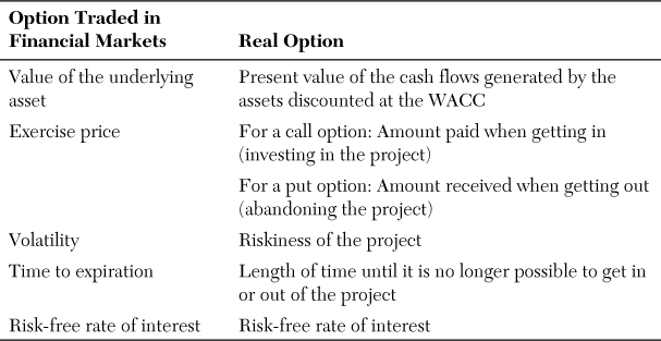
We return to our earlier example to illustrate how Company B could value the chain of restaurants:²⁵

• The value of the underlying asset would be the present value of the FCFs generated by the chain of restaurants discounted at the WACC for the restaurant division.

• The exercise price would be the cost of acquiring the chain of restaurants, including the purchase price and any costs associated with the transaction (excluding financing costs).

• The volatility would be the standard deviation of the FCFs generated by the chain of restaurants, based on historical data.

• The time to expiration would probably be relatively short, particularly if other companies or investors were interested in purchasing the chain of restaurant.

• The risk-free interest rate would be the yield-to-maturity on sovereign bonds with short maturities.

Academicians have studied real options for more than 30 years, but their use in the context of corporate valuation in general and M&A valuation in particular has been limited. A survey conducted by Baker, Dutta, and Saadi (2011) in Canada showed that real option analysis was the least popular valuation method. Of the 214 respondents, 80.9 percent admitted they had never used real option analysis. When asked why, they cited the lack of knowledge and expertise, the lack of applicability to their business, and the complexity to apply in practice. Respondents who used real option analysis viewed it as an opportunity to help form the strategic vision, incorporate managerial flexibility into the analysis, and provide a way of thinking about uncertainty and its effect on valuation over time.

Real option analysis is rarely appropriate as a stand-alone valuation method. It is too simplistic to model a target as a single option; instead, a target must be viewed as a portfolio of options. The problem is, estimating the parameters of each option in the “portfolio” is difficult, and some of the options might interfere with each other. In addition, not all assets and projects are real options. Real options analysis works best when there is uncertainty and investments occur in stages. For example, it is better suited to and more widely used in industries that have clear development or production stages, such as in the natural resources, real estate, or pharmaceutical industries.²⁶ It may also be used when there are multiple rounds of financing, which frequently characterizes the financing of new ventures. Alternatively, real option analysis can be used as an add-on to other valuation methods, such as the DCF models.

None of these valuation methods has challenged the domination of earnings multiples and the FCF to the firm model, but each might offer either a substitute or a complement to traditional valuation methods. Although highly risky as valuation methods, the P/Sales ratio and the EV/Sales multiple are better alternatives to the P/E ratio when a company has no current earnings or cash flows and is not expected to become profitable in the foreseeable future. The APV model is superior to the FCF to the firm model when a company’s capital structure is not stable. The FCF to equity model is more appropriate when an acquirer is seeking not control, but only a participation in the target. Economic value analysis might be a better approach when the forecasting period is too short to capture the long-term, sustainable level of capital investments. As for real option analysis, it complements DCF models when valuing investments that have option-like features.

In Chapter 5, we consider a variety of accounting and reporting dilemmas that analysts must resolve before using the valuation framework discussed thus far.

2. The P/Sales ratio of 9.4 times reported in the vignette was calculated by dividing the amount Cisco paid for Pure Digital ($590 million for the company’s equity plus $15 million in retention-based equity) by the revenues in the latest publicly available financial statements ($64.1 million). Based on the revenues that Pure Digital generated in 2008 ($145.6 million), the P/Sales ratio is 4.2. Although it is lower than the 9.4 times mentioned in the vignette, it is still much higher than our estimate of the average P/Sales ratio (1.5).

3. Under International Financial Reporting Standards (IFRS), it is possible to periodically revalue those assets whose values are affected by inflation. However, as discussed in Chapter 5, the analyst should check that the value of an asset that has been revalued does not exceed its fair market value.

4. Luehrman (1997) notes that other side effects include the costs of financial distress, subsidies, hedges, and issue costs.

5. Many analysts use Equation 4.2 to estimate the unleveraged beta. However, it is a biased estimate of the unleveraged beta because it assumes that the company’s debt is risk free. A precise estimate is given by:

where β_D is the beta of the company’s debt.

6. For example, Ruback (2002) advises discounting the ITSs at the cost of unleveraged equity, which leads to a variant of the APV model sometimes referred to as the compressed APV model or capital cash flow model. For a review of the different discount rates that are used in practice, see Ehrhardt and Daves (2002).

7. Deferred coupon bonds, or PIK coupon bonds, are typically issued by companies that may not generate sufficient cash in the years following issuance to service their debt. A deferred coupon bond does not make interest payments in the early years, but then makes higher interest payments than a conventional coupon-bearing bond. A PIK coupon bond gives the issuer the opportunity to make interest payments in securities (such as debt or equity securities) instead of cash. They are commonly used in LBOs.

8. All the calculations were performed in Excel, without rounding any of the intermediate results. Thus, slight differences might arise between the numbers reported and the ones obtained with a calculator.

9. Note that, under these assumptions, the calculation of the continuing value depends on only two variables: the amount of debt and the tax rate. The interest rate is irrelevant because it is included in both the numerator and denominator. This result leads us back to Modigliani and Miller’s Proposition I (1963), where the value of the leveraged company is equal to the value of the unleveraged company plus the amount of debt times the tax rate.

10. Because the famous Modigliani and Miller articles relate to capital structure (1958, 1963) and dividend policy (1961), i.e., financing decisions, many people misunderstand their message. As Miller stated (1988, 100): “The view that capital structure is literally irrelevant or that ‘nothing matters’ in corporate finance, though still attributed to us (...), is far from what we ever actually said about the real world applications of our theoretical propositions. Looking back now, perhaps we should have put more emphasis on the other, more upbeat side of the ‘nothing matters’ coin: showing what does not matter can also show, by implication, what does.” What matters is a company’s ability to create value from its operations.

11. See Petitt and Mathis (2011) for an example of a failed LBO, including a detailed valuation of the target (Masonite International Corporation) using the APV model.

12. This definition assumes that the company has only debt and common equity in its capital structure. If it also has preferred equity, then preferred dividends and redemptions of preferred shares must be subtracted and issuances of preferred shares must be added.

13. For simplicity, we consider only Mattel’s debt obligations to move from the FCFs to the firm to the FCFs to equity.

14. Because Mattel will pay down $50.0 million of debt in 2012, there will technically be a change in capital structure. However, this change is small, hence the reason we assume that the cost of equity will remain constant between 2011 and 2012; the effect of this small change on the cost of equity is insignificant. If the change were significant, the cost of equity would have to be recalculated. To do so, we would have to follow the approach described in Chapter 3, i.e., unleveraging Mattel’s beta using the debt-to-equity ratio for 2011 and then releveraging the beta using the debt-to-equity ratio for 2012.

15. The FCF to the firm, APV, and FCF to equity models are equivalent, so in theory, they should lead to the same equity value per share. In practice, this is rarely the case, primarily because of differences in assumptions. In the case of Mattel, assuming that the FCF to equity increase at 3.0 percent per annum is not identical to assuming that the FCF to the firm increase at 3.0 percent per annum; these two assumptions have different implications regarding the company’s marginal changes in capital structure.

16. Stern Stewart’s definition of EVA is similar to the definition in Equation 4.6. However, because their model is at the root of their consulting services, they do not disclose all the adjustments they make to value a company or one of its divisions.

17. In Chapter 3, we mentioned that the WACC should be calculated based on a company’s market values of debt and equity. However, because economic income models rely on information in the financial statements, practitioners who use the economic value analysis commonly calculate the WACC based on the book values of debt and equity.

18. Invested capital is defined in two ways, depending on whether it is viewed from the left side or the right side of the balance sheet. Total assets is the sum of cash and marketable securities, operating assets that are part of working capital (accounts receivables, inventories, and prepaid expenses) and net fixed assets. Total liabilities and equity is the sum of operating liabilities that are part of working capital (accounts payable and accrued expenses), interest-bearing debt (short-term debt, the current portion of long-term debt, and long-term debt), and stockholders’ equity. An alternative way of organizing a balance sheet is to view the left side as cash and marketable securities plus working capital (operating assets minus operating liabilities) plus net fixed assets, and the right side as interest-bearing debt plus stockholders’ equity; this balance sheet is sometimes called the managerial balance sheet. Thus, invested capital can be defined at the sum of the book values of debt and equity, as in the text. The term capital employed is sometimes associated with this definition. Alternatively, invested capital can be defined as the sum of cash and marketable securities, working capital, and net fixed assets. The term net assets is often associated with this definition, and it can also be defined as total assets minus accounts payable and accrued expenses.

19. It is also called return on net assets (RONA) or return on capital employed (ROCE) when the terms “net assets” or “capital employed” are used instead of “invested capital”.

20. The reason economic value analysis requires estimating the discount rate first is that the WACC is instrumental in the calculation of economic income, as shown in Equations 4.6–4.9.

21. Economic income models can be derived from DCF models such as the dividend discount model (DDM) with the assumption of clean surplus accounting. Clean surplus accounting holds when the income statement for the period reports all the transactions that affect the book value of equity during the period, other than transactions with equity holders. FASB Statement No. 130 requires that all items that violate clean surplus accounting be reported as comprehensive income. Under IFRS and U.S. Generally Accepted Accounting Principles (GAAP), companies usually report comprehensive income in the statement of shareholders’ equity or in a footnote to the financial statements.

22. For a comparison of residual (economic) income models and DCF models, see Penman and Sougiannis (1998).

23. The same individual, Stewart Myers, developed the APV model and applied the option pricing theory to real investments. For a review of the many contributions of Myers to the theory and practice of corporate finance, see Allen, Bhattacharya, Rajan, and Schoar (2008).

24. Equation IV in the appendix in Chapter 3 comes from Myers (1977): The value of a company can be viewed as the value provided by its assets in place plus the net present value of its growth opportunities.

25. Appendix 4 shows how to value such a real option with the Black-Scholes model.

26. For example, a survey conducted by Hartmann and Hassan (2006) shows that approximately a quarter of the companies in the pharmaceutical industry use real option analysis at different research and development stages (clinical Phases I to III). However, none of these companies applies it to value acquisition targets.

This investment opportunity can be viewed as an option to expand, a call option. To value this option, Company B’s advisers can use real option analysis. The value of the underlying asset (the restaurant division) is the present value of the FCFs generated by the restaurants discounted at the restaurant division’s WACC:

The exercise price is the amount paid to acquire the restaurant division, $100 million. The volatility is 30 percent, the time to expiration is three months, and the risk-free rate of interest is 5 percent.

An analyst has various ways of estimating the value of this call option. A first approach involves using the formulas associated with the Black-Scholes model. A second approach is to use the NPVq/cumulative volatility approach suggested by Luehrman (1998). The third approach is to build and/or use a financial model in Excel. These three approaches are equivalent; in this appendix, we present the first two.

C = S × N(d₁) - E×e^-rxt × N(d₂)

where S is the value of the underlying asset, E is the exercise price, r is the risk-free rate of interest, t is the time to expiration, and:

And:

Based on our example:

And:

Thus:

N(d₁) = 0.9979

And:

N(d₂) = 0.9967

Therefore:

The NPVq is similar to the profitability index, which indicates how much value is created per dollar of initial investment. The only difference is that the profitability index uses the amount of initial investment in the denominator, whereas the NPVq uses the present value of this amount. Thus, there is a need to discount the amount of initial investment. For the discount rate, some analysts use the WACC, which reflects the opportunity cost for a company or one of its divisions. However, because the Black-Scholes model assumes that discounting is done at the risk-free rate of interest, the result obtained when discounting at the WACC differs from the result obtained when discounting at the risk-free rate of interest. To demonstrate that no difference exists between Luehrman’s approach and the Black-Scholes model, we discount the initial investment at the risk-free rate of interest:

Therefore, the NPVq is:

The second component is the cumulative volatility, which is equal to:

In our example:

Luehrman (1998) provides a table that gives the value of a call option as a percentage of the value of the underlying asset. Based on an NPVq of 1.5 and a cumulative volatility of 0.15, the percentage is approximately 33.3, which means that the value of the call option is:

C = 33.3% × 150 = $50 million

The difference between the two approaches is due to a rounding error; the percentage provided in the table is only an approximation.

Luehrman (1998) also uses the analogy of a tomato garden to interpret the results of the NPVq/cumulative volatility framework. In our example, the call option is “in the money”—that is, the NPVq is greater than 1, indicating that the project would create value if launched today. The volatility is low, primarily because Company B has only three months to make a decision. Thus, Company B could exercise now and make an offer for $100 million.

As mentioned in the text, real option analysis is more valuable when there is a high level of uncertainty (high volatility), even more so when the length of time is long.