
5. Cost of Capital
5.1 Introduction
As stated in Chapter 1, “Introduction,” the primary goal of this book is to develop the methodology for measuring the value of any business decision, ranging from decisions such as going forward with a project (such as a new product introduction) or to acquisition decisions (such as purchasing another business). To do this, we need to evaluate the following present value relation:
where E(CF1), E(CF2), and so on are expected future cash flows, r denotes a discount rate, and Value0 is the value of the project that we are trying to measure. Chapter 4, “Free Cash Flows,” discussed how the numerators in this formula are computed. Each year we construct projected financial statements for the project that we are interested in valuing, and we then calculate free cash flows from these financials. The free cash flows are the numbers that are used in the numerator in the present value equation.
There is now only one piece missing: the denominators. This chapter shows how to compute the denominators in Equation 1. The basic idea is that the denominators represent discount rates, or expected rates of return. In general, rates of return correspond to risk. The higher the risk, the higher the rate of return. The rate of return in the denominator of any particular term in Equation 1 corresponds to the risk of the free cash flow in the numerator of that term. Hence to determine the discount rates needed for Equation 1, we will have to define risk and develop a relationship between risk and return. Then, all we have to do is to measure the risk of each projected free cash flow for the specific project we are evaluating, and we will use this risk-return relationship to determine the corresponding return, which we can plug into the denominator of the term in Equation 1 containing that free cash flow.
5.2 Risk and Return
If one were to invest in a zero-coupon, one-year U.S. Treasury bill that cost $95 and paid $100 in one year, the expected return on this security would be
Of course, because this is a risk-free security,1 the expected return of 5.26% will also be the realized return on the security. However, all securities, with a very few exceptions such as U.S. Treasuries, contain risk. What this means is that a typical security contains risk for the investor. Suppose, for instance, that the one-year bond previously described was issued by a corporation rather than the U.S. Treasury. Suppose also that this company has a 10% chance of defaulting in the next year, and if the company defaults, the bondholder will receive only $95. Due to the uncertainty of whether the company will default in the coming year, suppose that investors are now willing to pay only $93 for this security. The expected return of this security is now
Notice that the expected return for the corporate bond is higher than the Treasury bond. This is because of the uncertainty due to default. Investors are asking for a higher expected return because they are bearing greater uncertainty, or risk, about the possible payout of the bond one year from now. Investors get this higher expected return by paying a lower price for the bond today. The difference in expected return between the risky corporate bond risk-free Treasury bill is called a risk premium. In the preceding example, the risk premium paid by the corporate bond to investors is 6.99% – 5.26% = 1.73%.2 The risk premium for a Treasury security is 0% (because there is no possibility of default). This reveals an important concept about risk and risk premium. As risk increases, so does the risk premium; i.e., as investors bear more risk, they command a higher risk premium. This is perhaps the most fundamental principle of finance.3
For the purposes of evaluating Equation 1, we need to be able to calculate the expected return of all assets (including traded securities, like the corporate bond above). The difficulty is that for nearly all risky assets, including corporate bonds, it is difficult to evaluate the amount of risk in that asset. In the previous example, we stated that the risk of a default by the company is 10% and that investors would receive $95 at maturity in the case of a default. In reality, these are statements about the future, and therefore we would have a very difficult time quantifying exactly what the probability of default is and what the payoff in the case of default would be.4 So, we have to figure out a way to calculate the risk and expected returns for assets without knowing precisely all the potential future scenarios and payoffs in those scenarios.
The first step is to develop a way to measure risk. What makes a security risky is uncertainty to the investor about the payoff resulting from holding that security. In the preceding example, we assumed that the investor would hold the corporate bond to maturity, and the bond would pay either $100 or $95. The uncertainty of whether he receives $100 or $95 is defined as risk. However, the investor may decide to sell the security to a second investor before maturity. In this case, how much would the first investor receive for the sale? This is unknown. Many things may change in the economy, the company, the markets, and so on between now and the time of the sale. All of these changes would likely cause the second investor to attach a different probability of bankruptcy and different payoff if bankruptcy occurs to the corporate bond, which would result in a different price for the bond. This, too, represents risk to the first investor. The payoff to this investor from holding this bond is the sale price to the second investor, but this sale price is unknown, and therefore risky. So, the possibility of movement at any time in the price of assets one is holding represents the true risk of that asset. These price movements will generate varying returns to the investor in that asset. Therefore, rather than using prices, we can re-express risk in terms of returns: the possibility of generating variable returns from holding an asset represents the risk of that asset.
How do we measure the degree of variability in the returns that an asset produces? We use the simple statistical concept of standard deviation. Suppose that we have a stock and we are interested in measuring its risk. Suppose that in each of the past four months, the stock has produced the following returns: 4%, –3%, 5%, 2%. The risk of the stock is measured by the variability of the stock’s returns that an investor would face. We will measure this variability by calculating the standard deviation of the stock’s returns over the past four months. First, the mean return for the stock over the past four months is
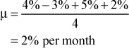
We use μ to denote the stock’s mean return. Normally, we quote mean returns on an annualized basis. Therefore, the stock has an average return of 24% per annum.5 We can now calculate the standard deviation of the stock:

We use σ2 to denote variance. The standard deviation, σ, is therefore
Just as with average return, we typically quote standard deviation, or volatility, on an annualized basis. The annualized volatility of the stock is therefore ![]() . We now have a way of measuring the risk of a stock.
. We now have a way of measuring the risk of a stock.
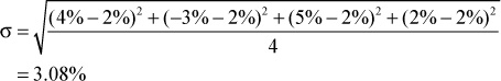
We will present one more investment concept, which we will need in subsequent sections. To gauge the value of a stock, it is not enough to know just the risk. The risk is simply the cost that investors have to pay (or bear) to gain the benefits from holding the stock. The benefit is the expected return. To do cost-benefit analysis of stocks and other assets, we would like to have a single metric that captures both the cost and the benefit of holding an asset. Many such metrics exist, but the simplest one is the Sharpe ratio:
For any asset A, the Sharpe ratio, SA, of that asset is defined as that asset’s expected return, μA, minus the risk-free rate, Rf, divided by the asset’s volatility, σA. The numerator of this equation is the asset’s risk premium, and the denominator is the risk of the asset. Therefore, the Sharpe ratio for any asset gives us that asset’s benefit per unit of risk for the investor that owns the asset. Obviously, higher Sharpe ratios are always more desirable for investors.
In the example above for the stock, if the risk-free rate is 4% per annum, and the stock’s mean return of 24% also represents its expected return, the Sharpe ratio of the stock is given by

Figure 5.1 presents a graphical way of thinking about the Sharpe ratio. This figure contains a risk-return graph. The horizontal axis represents the level of risk, and the vertical axis represents the level of expected return. Any asset in the investment universe can be placed as a point in this graph depending on its risk and expected return. The graph shows as an example of a stock with a volatility level of 10% and an expected return of 12%. There is also a risk-free asset with a volatility of 0% and an expected return of 2.5%. The Sharpe ratio of this stock is simply the slope of the line passing through both the risk-free asset and the stock. In general, the Sharpe ratio of any asset is the slope of the line passing through both that asset and the risk-free asset.
5.3 Risk Reduction through Diversification
An important question that we need to answer is what happens to the risk an investor bears when he owns more than one type of asset. In addition, a more important question is what happens to the Sharpe ratio of the investor’s portfolio when he holds more than one type of asset. This section answers these questions, which will then set up the next two sections concerning how to generate a discount rate, or required rate of return, for any asset.
Because we are using the statistical property of standard deviation to measure an asset’s risk, we can simply extend this approach to calculate risk when there is more than one asset. Suppose we have two assets, A and B, in a portfolio. Asset A has an expected return of μA and a volatility of σA. Meanwhile, asset B has an expected return of μB and a volatility of σB. What is the expected return and volatility of an investor’s portfolio if he holds both A and B? To answer this, we need two more pieces of information. First, we need to know how much the investor has invested into each of A and B (i.e., what fraction of the portfolio contains A and what fraction contains B). Suppose that wA represents the fraction of the investor’s portfolio invested in asset A, and wB represents the fraction invested in B.6 The second piece of information that we need is the relationship between the price movements of A and B; e.g., when A moves up 1%, what is B likely to do? We will use the statistical property of correlation to describe this relationship. We assume that A’s returns and B’s returns have a correlation of ρ. We can now state the expected return and volatility of the portfolio. The expected return of the portfolio is given by
where μP denotes the expected return of the portfolio. The volatility of the portfolio is given by
where σP denotes the portfolio’s volatility.
It is easiest to understand these formulas through an example. Suppose that we start with the stock in the example in the previous section. This stock had an expected return of 24.0% and a volatility of 10.7%. As we calculated earlier, the Sharpe ratio of this stock is 1.87, assuming a risk-free rate of 4%. Suppose that we also have a second stock with an expected return of 15% and a volatility of 12%. The Sharpe ratio for this stock is (15% – 4%) / 12% = 0.92. Assume that the correlation between the two stocks is 0.1.
Initially, it might not appear to make any sense to invest in stock 2. After all, why should one invest any money in a stock with a Sharpe ratio of 0.92 when one could instead invest in a stock with a much higher Sharpe ratio of 1.87. Putting some of the portfolio into the lower Sharpe ratio stock would seemingly only lower the Sharpe ratio of the portfolio down from 1.87.
Let’s check this intuition by putting 70% of the portfolio into stock 1 (the higher Sharpe ratio stock) and 30% of the portfolio into stock 2. Plugging these values into Equations 3 and 4, we can calculate that the portfolio has an expected return of 21.3% and a volatility of 8.6%. This means that the portfolio has a Sharpe ratio of 2.0. Contrary to what our intuition may have suggested, the Sharpe ratio of the portfolio went up rather than decreasing below the Sharpe ratio of stock 1 alone.
The key to the increase in Sharpe ratio is the fact that the volatility of the portfolio of the two stocks actually decreased below the volatility of each of the individual stocks. This occurs because of the low correlation between the two stocks. This low correlation means that when one stock goes up, the other has a good chance of going down. And vice versa, when one stock goes down, the other has a good chance of going up. Therefore, due to the low correlation, one stock always has a good chance of counteracting the movement of the other stock. This offsetting of individual stock price movements means that the movement of the portfolio as a whole decreases. The result is a lower volatility for the portfolio of the two stocks than for either stock individually. We call this effect diversification. Due to diversification, the volatility of the portfolio drops substantially. Meanwhile the expected return is simply a weighed average of the two individual stocks. As a result, the Sharpe ratio of the portfolio increases.
Figure 5.2 uses the risk-return graph presented in the previous section to demonstrate what happens as we move from a portfolio that is 100% invested in stock 1 to a portfolio that has a mix of stock 1 and stock 2 to a portfolio that is 100% invested in stock 2. The curved line represents the risk-return point of the portfolio as it moves gradually from a 100% investment in stock 1 to a 100% investment in stock 2. The slopes of the straight lines represent Sharpe ratios of the portfolio when it 100% invested in stock 1, when it contains a mix of stock 1 and stock 2, and when it is 100% invested in stock 2. Due to the diversification effect, the Sharpe ratio starts increasing as we start with the 100% stock 1 portfolio and add more and more of stock 2. At some point, however, the portfolio begins to contain mostly stock 2, and the Sharpe ratio starts decreasing. Notice that there is a mix of stock 1 and stock 2, which maximizes the Sharpe ratio. At this point (as well as neighboring points), the Sharpe ratio of the portfolio is higher than the Sharpe ratio of either stock 1 alone or stock 2 alone.

The principle of diversification is one of the most important principles of investing. It says that achieving a high Sharpe ratio is not just about investing in stocks that have high expected return and low volatility (i.e., high Sharpe ratios). It is also about investing in stocks that have low correlations with other stocks. Due to the effects of diversification, these low-correlation stocks will drive the volatility of the portfolio substantially lower, thus increasing the portfolio’s Sharpe ratio above what one could achieve with an investment in high Sharpe ratio stocks alone.
5.4 Systematic Versus Unsystematic Risk
Due to the principle of diversification, if we place two uncorrelated (with correlation less than one) assets in a portfolio, the risk of the portfolio can be lower than that of either individual asset. Furthermore, the Sharpe ratio of the portfolio will be higher than the Sharpe ratio of either individual asset. This is because the less-than-perfect correlation between the two assets means that some of the variation of one asset will be counteracted by some of the variation of the second asset, thereby dampening the volatility of the portfolio.
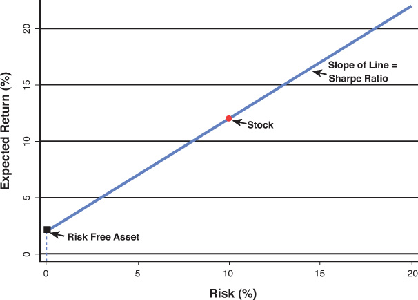
We can carry the diversification principle further. Suppose that we take this portfolio of two assets and we add another asset to it. The same principle applies. We can reduce the volatility of the portfolio and increase its Sharpe ratio. Now, we can repeat this again. We can add a fourth asset to the portfolio and reduce its volatility and increase its Sharpe ratio. In fact, we can keep adding assets to the portfolio, and as long as the assets being added are less than perfectly correlated with the portfolio, the addition will lower the volatility of the portfolio a bit more and increase its Sharpe ratio a bit more.
So, how far can we lower the volatility of the portfolio? Figures 5.3 and 5.4 shows what happens as we keep adding assets to the portfolio. As we add more and more assets, the volatility of the portfolio converges to a lower bound, and the Sharpe ratio of the portfolio converges to an upper bound. The lower bound and upper bound are achieved essentially when every asset in the investable universe has been added to the portfolio. This portfolio, therefore, is called the world market portfolio, and the volatility of the market portfolio (the lower volatility bound) is known as market volatility, or market risk.

Another name for market risk is nondiversifiable risk. For any individual asset in the world market portfolio, the bulk of its risk is diversified away by all the other assets in the portfolio. As we add more and more assets to the world market portfolio, the total risk of any individual asset decreases until it contains only its contribution to market risk. Because there are quite a lot of investable assets in the world, an individual security’s remaining risk after diversification (its market risk contribution) is nearly the same as market risk. Therefore, we tend to think of the total risk of any individual security as composed of two pieces: a diversifiable component (i.e., diversifiable risk) and a market component (i.e., nondiversifiable risk).
Market-related risk cannot be diversified away by an investor no matter how much he diversifies his portfolio. It is risk that is inherent to the global economic system. Therefore, investors also refer to this form of risk as systematic risk (and to diversifiable risk as nonsystematic risk). Examples of risk inherent to the global economic system would be the risk of a world war, an international trade dispute, an increase in the yield curve, and the introduction of new computer technology. Examples of nonsystematic risk include the risk of an individual firm’s CEO dying, the sudden departure of an individual firm’s star salesperson, and a union strike at an individual manufacturing plant. Notice that in the examples of nonsystematic risk, the risks are typically specific to an individual firm. That is because these risks are completely uncorrelated to the global economic system and therefore are easily diversified away. For this reason, other names for diversifiable risk include firm-specific risk and idiosyncratic risk.
5.5 The Capital Asset Pricing Model
Just as the volatility of the world market portfolio is a lower bound, the Sharpe ratio of the world market portfolio is an upper bound and is known as the market Sharpe ratio. The market Sharpe ratio plays a special role in the determination of the cost of capital for any investable asset.
As discussed in the preceding section, when we add an asset to the world market portfolio, that asset’s diversifiable, or nonsystematic, risk gets diversified away. This leaves only the systematic risk of that asset. Therefore, when an investor invests in an asset, if he holds only that asset, then he bears total risk, both nonsystematic and systematic risk. However, if the investor holds the market portfolio and invests in that asset and adds it to his market portfolio, then he bears only systematic risk. We discussed earlier that as an investor bears more risk, he needs to be paid a higher rate of return, or risk premium, to compensate him for that higher risk. So, then the question naturally arises as to which is the relevant risk—systematic, nonsystematic, or total risk—for which he should earn a risk premium.
If we think of a risk premium as a reward for bearing risk, then we should only reward an investor for bearing risk that needs to be borne (i.e., that some investor in the world needs to bear because it cannot be eliminated). The answer then is very simple. The relevant risk of any asset is its systematic risk. The nonsystematic risk in any asset can be easily eliminated by any investor by simply diversifying his portfolio. Therefore, both nonsystematic risk and the nonsystematic component of total risk can be eliminated. Systematic risk cannot be eliminated; it must be borne by somebody. Therefore, the market rewards an investor who is willing to bear the systematic risk in an asset by paying a risk premium. How much of a risk premium does the market pay for holding an asset?
The risk premium for any security should be tied to the amount of systematic risk in that asset. Let’s start with the easiest asset: the world market portfolio. The world market portfolio only contains systematic risk (because all nonsystematic risk has been diversified away). Suppose we define the market Sharpe ratio (the Sharpe ratio of the world market portfolio) as SM. So, we can conclude that for pure systematic risk, an investor earns a risk premium per unit of systematic risk (recall that this is the definition of a Sharpe ratio) equal to SM. Now let’s consider the case of an asset that is not the world market portfolio. The market pays a risk premium for only the systematic risk in that asset. How do we measure the systematic risk in an asset? We can simply measure the correlation of that asset to the world market portfolio. If the correlation is one, then the asset contains only systematic risk and its Sharpe ratio should be the same as that of the world market portfolio. If its correlation is zero, then it contains no systematic risk, and its Sharpe ratio should be zero; i.e., the market should not pay any risk premium to an investor for holding this asset because the asset contains only nonsystematic risk. If the correlation is something other than one or zero, suppose it is ρA, the Sharpe ratio of the asset, SA is given by
This equation just states that the Sharpe ratio of any asset is equal to the correlation of that asset with the world market portfolio times the Sharpe ratio of the world market portfolio, SM. Notice that if the correlation is zero or one, we get precisely the Sharpe ratio that we described earlier.
We will now expand this equation by explicitly writing out the Sharpe ratio as the ratio of the risk premium of an asset and its volatility:

where RA and σA denote the asset’s expected return and volatility, RM and σM denote the world market portfolio’s expected return and volatility, ρ denotes the correlation between the asset and the world market portfolio, and Rf denotes the risk-free rate. We can rearrange this equation to obtain the risk premium for the asset:

For simplicity, we will denote the term ![]() as simply as βA.
as simply as βA.
This equation is known as the capital asset pricing model (CAPM), and it enables us to calculate the risk premium of any asset. The term βA is known as the beta of an asset, and it is a measure of the systematic risk in an asset. Therefore, the higher the beta, the higher the risk premium the market pays for an asset. Examples of low beta assets would be the stock of a utility or a food company. Regardless of what happens in the global economic system, consumers are unlikely to change the consumption of gas, electricity, or food by very much. Therefore, these stocks would have low correlations with the world market portfolio, which would result in a low betas (typically around 0.6 or 0.7). Conversely, the stock of a business equipment manufacturer or a steel producer would tend to have a high beta. If a downturn in the global economy occurs, businesses tend to cut back on production, and there is less office construction, which in turn leads to lower demand for business equipment and steel, respectively. By the same argument, in a global economic upturn, demand for these products would be high. Therefore, these stocks tend to be highly correlated with the world market portfolio. As a result, their betas tend to be high (typically around 1.2 or 1.3).
As an example, let’s calculate the risk premium for the stock of a food manufacturer with a beta of 0.7. With the β known, the only thing that we have to calculate is RM – Rf, the world market risk premium. Of course, we would like to calculate the expected risk premium for the world market going forward. However, we have no way of looking into the future. Instead, we will do the best we can by utilizing historical data on the world market risk premium. We need to collect data on all of the world’s markets, which presents a major challenge. Data on the U.S. markets exist for over a hundred years, but most asset markets in the world have existed (or we only have satisfactory data on them) for only one or two decades at best. Because we are going to use historical data to estimate an expected return, we would like to have historical data going a long way back.7 In practice, we get around this problem by using the U.S. equity markets as a proxy for the world market portfolio. Due to the multinational nature of many U.S. companies and due to the enormous global diversity of asset holdings of U.S. companies, the U.S. equity market should be a fair proxy for the world asset market. So, we will take historical yearly returns of the U.S. equity markets and each year we will subtract off the 1-year return of a long-maturity Treasury bond (typically a 30-year bond) during that year. This produces a historical time series of RM – Rf. (The RM is proxied each year by the U.S. equity market return for that year, and Rf is proxied by the return produced the long Treasury bond during that year.) We can average this time series, which should produce a reasonable estimate of the going forward world market risk premium. This premium turns out to be approximately 6%. So now, we can calculate the risk premium for the stock of the food manufacturer.
RA – Rf = 0.7 × (6%) = 4.2%
The risk premium is 4.2%. If the current risk-free rate is 4.0% (this is the yield on a 30-year Treasury bond), we can calculate the expected return to an investor for holding the manufacturer’s stock:
RA – Rf = 4.2%
RA = 4.2% + Rf
= 4.2% + 4.0%
= 8.2%
Thus, the expected return to an investor for holding this stock is 8.2%.
One might wonder why it is necessary to use the CAPM to calculate the expected return for an asset rather than simply averaging that asset’s historical returns. The reason for this goes back to the discussion earlier about using historical returns to compute an expected market risk premium. Quite a lot of historical data is needed for the average to produce a good estimate (with low standard error) of the going forward expected return. However, the vast majority of assets such as publicly traded firms have not been in existence for a long time (or its returns have been available/observable for only a short period of time). For this reason, it is much more convenient to use historical data on the market (for which a long time series exists) and link the market to the asset for which we are interested in calculating an expected return. The critical information that allows this link is the β of the asset. Notice that the β only requires the calculation of second moments (correlation and volatilities); it does not require the calculation of an expected return (a first moment). A convenient statistical property about producing a good estimate (low standard error) for second moments is that its precision depends on the frequency of the historical data rather than the length of historical data (as first moments depend on). Therefore, as long as we use reasonably high frequency data (monthly or higher frequency) to calculate the β, we should be able to produce a good estimate for β. Thus, we have a way to produce good estimates for the market risk premium and the β of an asset with respect to the market. This is why we employ the CAPM to estimate expected returns for assets.
One might also wonder how to calculate a β for an asset. For many publicly traded securities such as equities, the β can be obtained from financial information services such as Bloomberg and Compustat. However, if it isn’t available through such services, one can always calculate a β for an asset manually by running a regression of the asset’s historical excess returns against the market’s excess returns. The slope coefficient of such a regression is exactly the β that is needed in the CAPM.
5.6 The Cost of Capital for a Traded Asset
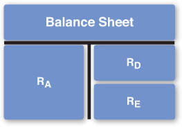
Now that we have discussed the CAPM, we are now ready to calculate the cost of capital, or discount rate, required in the present value equation, Equation 1. There are two situations to consider. First, we will consider the situation where we have an asset that is traded. If we consider the balance sheet representation for the asset, Figure 5.5, what this typically means is that the equity of the asset is traded.

When we implement the present value equation, we will match up the denominator to the numerator. What this means is that the cost of capital in the denominator will correspond to the riskiness of the cash flows in the numerator. We discuss this matching process and the details of implementing the present value equation in the next chapter. Therefore, in this section as well as the next one, we focus on calculating all three relevant costs of capital for a firm. These are the cost of equity capital (RE), cost of debt capital (RD) and the asset cost of capital (RA). These are depicted in Figure 5.6.
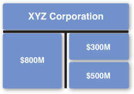
We will go through the calculation of all three of these costs of capital via an example. Suppose that XYZ Corp. has a market value balance sheet as shown in Figure 5.7. The value of its equity is $500M. Its debt has a market value of $300M. Because the balance sheet must balance, debt plus equity must equal asset value. Therefore, its asset value is $800M.
The cost of equity capital is fairly easy to calculate if XYZ is a market-traded firm. Essentially, we will calculate the cost of equity as we did in the previous section using the CAPM. Suppose that we find from financial information services or from our own regressions of XYZ’s stock price data that XYZ’s equity beta is 0.8. Then if the long bond yield is 4.0%, we have the following result for XYZ’s cost of equity:
= 4.0% + 0.8(6%)
= 8.8%
We are assuming the same 6% world market risk premium, which we stipulated in the previous section. Therefore, the cost of equity is straightforward to calculate.
The cost of debt is a bit trickier. The first thing to realize is that for most firms, the market value of debt is difficult to obtain directly. This is because most firms either do not have publicly traded debt or have only a small fraction that is publicly traded. This is because most debt tends to be short/long-term bank debt and other forms of private debt. Therefore, the first question we are faced with is how to simply calculate the market value of debt for a firm. No matter what form of debt the firm has, this debt must be recorded on the firm’s accounting balance sheet. Therefore, a commonly employed technique is to simply assume that the market value of debt is equal to the book value of debt recorded on the firm’s accounting balance sheet. This is a reasonable assumption. When debt is issued, it is typically issued at par value—so that the value recorded on the accounting balance sheet is also the market value at the time of issuance. The question then is how big of a mistake might we make if we are looking at a firm’s balance sheet, where all the debt on the books has been issued in the past. First, debt does not fluctuate in value as much as equities. This is because debt value is tied to interest rates, which are less volatile than equity prices. Second, interest rates tend to be mean-reverting, so that the market value of debt will probably fluctuate around par value. For these reasons, it can be argued that the error made by assuming that the market value of debt equals the book value of debt is not too bad. This is precisely how we arrived at the market value of debt for XYZ: $300M is the aggregate book value of this firm’s debt, and we are assuming this to be its market value.
Knowing the market value of debt is the first step. We need to figure out the firm’s cost of capital for this debt. Suppose that the firm’s weighted average yield on this debt is Yp. This yield is of course simply a promised yield (i.e., this is what the bond investor earns if the firm does not default). The cost of debt capital is the expected yield, which is what we need to calculate. The expected yield is a probability of default-weighted average of the promised yield and the yield a bond investor would get if the firm defaults:
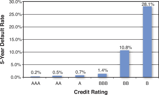
In this equation, Ye is the expected yield, or cost of debt capital, which is what we are after. The letter d denotes the default probability of the firm, and YL denotes the yield, or loss rate, in case the firm defaults. Suppose that the weighted average yield of XYZ’s debt is 5.5%. Suppose also that we know that XYZ’s debt has an average debt rating of BBB+.8 Then we can use information such as that given in Figures 5.8 and 5.9 to calculate the probability of default, d, and loss rate, YL. The information used to create these two figures is readily available from any of the major credit ratings agencies. From Figure 5.8, we can see that the average default rate for BBB-rated companies is 0.32% per year (1.6%/5 years). From Figure 5.9, if we assume that XYZ has mostly senior unsecured debt, the loss rate for XYZ’s debt is 1 – 48% = 52%. Therefore, we can now utilize Equation 11:
Ye = (1 – d) Yp + dYL
= (1 – 0.32%) 5.5% + 0.32% (–52%)
= 5.3%

Thus, the cost of debt capital, RD, for XYZ is 5.3%. A “back of the envelope” technique that is sometimes employed to estimate the cost of debt capital is to simply assume that a firm’s debt has a debt beta in the range of 0.1 to 0.5 and then to simply use the CAPM. The lower end of the beta range would be used for higher-quality (rated) firms, while the higher end of that range would be used for lower-quality firms. Let’s try this with XYZ. Because XYZ is BBB+ rated (which is in the middle to upper-middle portion of the credit ratings range), suppose that we assume that XYZ’s debt beta is roughly 0.2. We can now employ the CAPM:
RD = Rf + βD (RM – Rf)
= 4.0% + 0.2(6%)
= 5.2%
As you see, this quick-and-dirty approach produces a value that is close to the value we calculated through more precise means.
Now that we have calculated RE and RD, it is easy to calculate the asset cost of capital, RA. Using Figure 5.6, and the fact that a balance sheet must balance, we have the following formula for the asset cost of capital for XYZ:
This equation states that the asset cost of capital is simply the weighted average of the cost of equity capital and the cost of debt capital. The weightings are simply the debt-to-total capital ratio and the equity-to-total capital ratio. The simple intuition of why this formula works derives from the balance sheet representation of a firm. This formula simply states that the asset cost of capital is the (market capitalization) weighted average of the debt cost of capital and the equity cost of capital.9
For XYZ, the market value of debt is $300M, and the market value of equity is $500M. Therefore, we can calculate its asset cost of capital:

The asset cost of capital for XYZ is 7.5%. With this, we have calculated the costs of equity, debt, and asset capital for XYZ.
5.7 The Cost of Capital for a Nontraded Asset
We now take up the question of calculating the cost of equity capital, cost of debt capital, and asset cost of capital when the asset (specifically, its equity) is not traded (i.e., when it is a private asset). This is a typical situation. This not only applies to the valuation of private businesses but also the valuation of nearly any project. A project such as the introduction of a new product or a new marketing campaign is not traded. Therefore, the techniques discussed in the previous section become difficult to apply because we cannot measure the project’s equity, debt, and asset values. Nevertheless, it is important to understand that the balance sheet depiction of Figure 5.5 still applies to the project; the difference is that we simply cannot observe the market values of the balance sheet components.
The standard approach to dealing with unobservable information in finance is to utilize traded comparables, whether those are comparable firms, comparable securities, or so on. We will utilize the same approach here. What we will do is find a comparable traded firm whose business (asset side of the balance sheet) is similar to the private asset that we are interested in calculating discount rates for.
We will continue the example from the previous section. Suppose that we are trying to calculate the costs of capital for ABC Corp. Unlike we did for XYZ Corp. discussed earlier, let’s assume that ABC is nontraded. What this means is that we cannot observe its stock price movements through time. As a result, we cannot utilize the CAPM to determine a cost of equity capital as we did in the previous section. Instead, we will utilize the information that we have obtained from a comparable traded firm. We will assume that XYZ, the firm whose costs of capital we calculated above, is comparable to ABC. ABC’s market value balance sheet is shown in Figure 5.10. ABC’s equity has a market value of $1,200M, while its debt has a market value of $400M.10 Its asset value is, therefore, $1,600M.11

The key to determining ABC’s costs of capital is XYZ. XYZ is a comparable firm. What this means is that the business that XYZ is in is similar to the business that ABC is in. In the language of finance, what this means is that the left-hand side of XYZ’s balance sheet is similar to the left-hand side of ABC’s balance sheet. Therefore, if the assets of the two balance sheets are similar, the riskiness of the assets in the two balance sheets must be similar as well. Finally, if the riskiness of the assets of ABC is similar to that of XYZ, the asset cost of capital for ABC should be the same as the asset cost of capital for XYZ. Thus, we’ve determined that the asset cost of capital for ABC must be 7.5%, the same as what we calculated above for XYZ.
We cannot use this same argument for determining the cost of equity and cost of debt for ABC because the riskiness of the right-hand sides of ABC’s balance sheet and XYZ’s balance sheet are very different. XYZ’s debt ratio is 38%, while ABC’s debt ratio is 25%. The lower debt ratio for ABC means that it has a lower probability of defaulting. The lower probability of default implies that both the cost of debt and the cost of equity for ABC must be lower, reflecting the lower level of risk.
We can go through either of the approaches previously described to determine the cost of debt for ABC. To keep things simple, we will assume that the lower riskiness means that the debt beta for ABC is slightly lower than average, at around 0.15. This translates into a cost of debt of
RD = Rf + βD (RM – Rf)
= 4.0% + 0.15(6%)
= 4.9%
We can now figure out the cost of equity by applying Equation 12 again. The difference now is that rather than calculating the cost of assets, the unknown variable is the cost of equity. So, we will solve for that instead:

We can now solve this for the RE, the cost of equity for XYZ:

Thus, ABC’s cost of equity is 8.4%, which is less than XYZ’s cost of equity calculated earlier of 8.8%. Because ABC has less leverage than XYZ, its equity is less risky, and therefore the cost of its equity is lower. The key step in calculating ABC’s cost of equity was inverting the asset cost of capital formula, Equation 12, and solving for the cost of equity rather than the cost of assets.
To summarize, by using a comparable traded firm, we can calculate the costs of capital for a nontraded firm. The cost of assets for the nontraded firm will be the same as that of the traded firm because they are in similar businesses. Because we can safely assume that the book value of debt and market value of debt are fairly close, the cost of debt can be obtained through the same methodologies described in the previous section. Finally, the cost of equity can be obtained by inverting the asset cost of capital formula, Equation 12, and solving for the cost of equity of the nontraded firm.
5.8 The Asset Cost of Capital Formula
We mentioned when we first stated the formula for the asset cost of capital, Equation 12, that the derivation of this formula is not as simple as one might think. This section shows the details of the derivation of this formula. This will also give us an opportunity to introduce the notion of an interest tax shield and how this fits into the balance sheet representation of a firm.
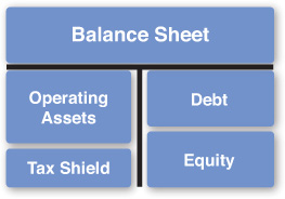
If we consider the balance sheet representations of the firm and the costs of capital for a firm, Figures 5.5 and 5.6, there is an important element that is not explicitly stated in these figures. Specifically, it is the fact that the presence of debt on a balance sheet introduces a tax shield into the balance sheet. This is because the interest expense on debt is tax deductible. The tax deduction results in an increase in cash flows for the firm by reducing the firm’s tax expense. Because this is a perpetual increase in cash flow, the value of this tax shield is worth much more than the increase in cash flow in any given year.
Figure 5.11 shows how the balance sheet view of a firm looks with this tax shield value included. The value of the tax shield, TS, shows up on the left-hand side of the balance sheet. Therefore, the assets are now split into two components. The first is the operating assets, OA, of the firm, which are used to derive the revenues for the business. The second is the tax shield.12 The two together sum to form the total assets, A, of the firm.
Based on Figure 5.11, we can now write a relationship between the costs of capital for a firm:
The discount rate of the tax shield is a function of the debt policy followed by the firm. At this point, we will discuss two types of debt policy: a fixed debt level policy and a fixed debt ratio policy. A fixed debt level indicates that regardless of what happens to the size of the firm’s assets and equity the firm intends to keep the same dollar amount of debt on the balance sheet going into the future. A fixed debt ratio policy indicates that the firm will maintain the same proportion of debt to assets on the balance sheet. Thus, with a fixed debt ratio as the level of assets increases or decreases, the debt level will increase or decrease, respectively, in such a way that the ratio of debt to assets remains the same into the future. Notice that a fixed debt ratio policy also implies that the ratio of debt to equity on the balance will also necessarily remain the same into the future.
We first take up the case of a fixed debt ratio. In this case, the amount of the tax shield is directly related to the level of debt on the balance sheet. The more debt there is on the balance sheet, the greater the tax shield. The less debt there is, the lower the tax shield. Therefore, the variability of the tax shield is directly proportional to the variability of the debt level. This in turn means that the riskiness of the tax shield, and therefore its discount rate, is directly proportional to the variability of the debt level. However, the debt level is tied to the asset level, and therefore the variability of the debt level is equal to the variability of the asset level. We can now tie these two pieces together. The variability (risk) of the tax shield must be equal to the variability (risk) of the asset level because the debt level is proportional to the asset level. Thus, the discount rate of the tax shield is equal to the discount rate of the assets: RT S = RA.
If the amount of the tax shield is small relative to the amount of operating assets in the firm, then the operating asset value is approximately equal to the asset value, OA = A. As a result, we can simply denote OA as A. Therefore, we can rewrite Equation 13 as
We can now combine the two fractions on the left-hand side of this equation:
Of course,![]() , and therefore we have
, and therefore we have
This is precisely the same formula as stated earlier in Equation 12. However, we see from the careful derivation of this equation that it only applies when the firm is following a policy of maintaining a constant debt ratio.
Now let’s consider the other debt policy: Suppose that the firm decides to maintain a fixed debt level rather than a fixed debt ratio. We start with Equation 13 again. However, with a fixed debt level, we can figure out the value of the tax shield precisely by utilizing Equation 1 to determine its present value. If we assume that the firm faces a tax rate of τ on its profits, then each year $1 of interest increases the after-tax cash flow by 1 × τ. This is because $1 of interest reduces earnings before taxes (EBT) by $1 and thereby shields $1 of EBT from taxation. If the tax rate is, for example, 35%, that $1 reduction of net income produces an extra $0.35 of earnings after taxes, or net income. So, each dollar of interest expense increases after-tax cash flow by τ dollars each year. We can use this information to calculate the total present value of the tax shield.
If the debt is at par value, the interest rate on the debt is equal to its market yield; therefore, the interest rate on the debt is RD. For simplicity, we will assume that interest is paid annually. The total annual interest payment that the firm makes on its debt is RDD, the interest rate times the principal amount of the debt. Because the debt level is fixed, this is the annual payment the firm makes on its debt into perpetuity. From above, we know that for every $1 of interest paid, the firm gets a tax shield of τ. Therefore, the annual tax shield into perpetuity is equal to RDDτ.
We can now use the present value formula, Equation 1, to calculate the present value of these annual tax shield benefits. The annual tax shield cash flow is given by RDDτ. The riskiness of this tax shield is equal to the riskiness of the debt because the debt level is fixed (unlike with a fixed debt ratio where the debt level varies with the asset level). Therefore, the discount rate on the annual tax shield is simply the discount rate on the debt, RD. The total tax shield value is then given by
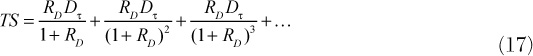
It is easy to simplify the right-hand side of this equation:13
We have therefore calculated the value of the tax shield. We can now go to Equation 13 and make two substitutions into this equation. First, we can replace TS with Dτ in the numerator of the second term. Second, we can replace RTS with RD because we know that the discount rate of the tax shield is simply the cost of debt (due to the fixed debt level policy). Third, we know that a balance sheet must balance, so we know that OA + TS = D + E. Therefore, we can replace OA + TS with D + E. These substitutions leave us with the following equation:
We can move ![]() to the right-hand side and consolidate terms.
to the right-hand side and consolidate terms.
As we did earlier with a fixed debt ratio policy, if we again assume that the tax shield value is small compared to the value of operating assets, then the operating asset value is approximately equal to the asset value, OA ≈ A. We can replace OA on the left-hand side with A:
The second line follows because ![]() . Thus, we have derived the asset cost of capital formula, Equation 23 in the case where the firm is following a fixed debt level policy. In this case, we use the after-tax cost of debt on the right-hand side of the formula. Notice that although it is very close to the asset cost of capital formula in the case of fixed debt ratio, Equation 16, it is nevertheless not the same. In Equation 16, we use the pretax cost of debt.
. Thus, we have derived the asset cost of capital formula, Equation 23 in the case where the firm is following a fixed debt level policy. In this case, we use the after-tax cost of debt on the right-hand side of the formula. Notice that although it is very close to the asset cost of capital formula in the case of fixed debt ratio, Equation 16, it is nevertheless not the same. In Equation 16, we use the pretax cost of debt.
In conclusion, we have to know which situation we are in before applying an asset cost of capital formula to a firm. If a firm is following a fixed debt ratio policy, we use the pretax cost of debt in the asset cost of capital formula. If a firm is following a fixed debt level policy, we use the after-tax cost of debt in this formula. In most cases, firms follow a policy of maintaining a fixed debt ratio, and therefore one would typically use Equation 16 for determining the asset cost of capital.14 This is precisely what we did in the examples in this chapter where we calculated firms’ costs of capital.
Endnotes
1. By risk free, we mean that in the case of this security, if you pay $95 and purchase this T-bill, you will receive the principal of $100 for sure in one year. Therefore, there is no possibility of default. Our working assumption throughout this book is that U.S. government-backed securities are the safest ones available in the entire investment universe. Therefore, we will treat all such securities as being free of risk over the life of those securities.
2. Note that this is not the same thing as a credit spread. The credit spread is the difference in promised returns rather than expected returns between the corporate bond and Treasury bill. The credit spread in this example would be
The credit spread does not factor in the possibility of default in the calculation of future payoffs. (Both payoffs in the earlier calculation assume $100 received at maturity.) Therefore, the credit spread is always higher than the expected return for bonds.
3. We hope this is fairly intuitive to the reader, as well. This principle is rooted in the microeconomics concept of concave investor preferences, which we do not delve into in this book.
4. We can always make qualitative statements such as “the company is unlikely to default,” but attaching a specific number to the probability of default is impossible.
5. Note that we are not taking into effect compounding here. The 24% is simply a quoting mechanism and not an expected return. The expected return is 2% per month, and 24% per annum is simply a way to quote the 2% per month.
6. Note that wA + wB = 1. So, we could also have stated the two weights as wA and 1 – wA.
7. This is due to a statistical characteristic of the first moments of any random variable, which is how we are modeling asset prices. To generate a reasonably accurate estimate (i.e., one with a low standard error) of the first moment of a random variable, a very long time series is needed.
8. We are using S&P credit ratings here. A rough equivalent in terms of Moody’s ratings would be Baa1.
9. Although this looks like it derives easily from the balance sheet representation of a firm, it is actually a bit tricky. This is due to the fact that debt on the right-hand side of the balance sheet introduces a tax shield into the balance sheet. We derive this formula more rigorously in the last section, Section 5.8, “The Asset Cost of Capital Formula.”
10. One can assume that this market value was calculated as it was done for XYZ previously; i.e., this is the book value of its aggregate long-term debt
11. Note that while we are assuming that we can determine the market value of equity today (we discuss in the next chapter how to do this), we do not know the historical movement of this equity price. It is because of this lack of time series information that we cannot calculate its equity beta and, therefore, its equity cost of capital directly.
12. Because the tax shield does not directly contribute to business revenue, we do not consider this asset as part of the operating assets.
13. We use the following general formula for the summation of an infinite series:
V = a + a(1+r) + a(1+r)2 + a(1+r)3 + ...
14. Notable exceptions include cases such as leveraged buyouts where a firm is following a policy of reducing debt according to a specific debt repayment schedule.