4. Free Cash Flows

where E(CF₁), E(CF₂), and so on are expected future cash flows, r denotes a discount rate, and Value₀ is the value today (time 0) of the project that we are trying to measure. Because all the cash flows and discount rates are expectations of future events, in the previous chapter we started the process of determining these expectations by figuring out how to project financial statements into the future. In this chapter, you learn how to use these projected financial statements to determine the numerators of Equation 1.

In Chapter 3, as we projected the income statement and balance sheet, we set up a “plug” account on the right-hand side of the balance sheet. This allowed us to balance the left-hand and right-hand sides of the balance sheet. For convenience, we considered the plug account as some form of debt; in Figure 3.1, we used long-term debt.¹

However, the plug can take on any flavor of financing. It could be short-term debt, long-term debt, equity, hybrid equity (such as preferred stock or convertibles), and so on. Therefore, a CFO has to determine not only the amount of financing that a business needs to finance its operations into the future, she must also determine what form this financing should take.² In general, the decrease in the financing amount (or plug account) needed each year to balance the left-hand and right-hand sides of the balance sheet is known as free cash flow.³ So, free cash flow is an indication of the amount of unused, or free, cash that is produced by the business. With the way we have been constructing our projected balance sheets so far, this free cash is automatically used to decrease, or pay off, the plug account (long-term debt in the balance sheet projections in Figure 3.1). This is why free cash flow can be measured by how much the plug account decreases.

From the work we have done so far, the free cash flow in any given quarter or year may be calculated as simply the decrease in the plug account on the right-hand side of the balance sheet. Referring back to Figure 3.1, we can examine the long-term debt line of the balance sheet to measure the decrease in the amount of the plug needed to bring the balance sheet into balance. For 2014, this amount was –($1,978M – $1,879M) = –$99M, for 2015 it was –($2,084M – $1,978M) =–$106M, and for 2016, –($2,200M – $2,084M) = –$116M. These negative free cash flows indicate that the business is not projected to produce free cash but instead it is expected to use up cash. As a result of this usage, additional debt has to be issued to raise this extra cash.

Figure 4.1 Graphical view of the meaning of free cash flow

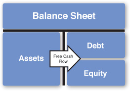
As we noted in Section 4.2, “Free Cash Flow Definition,” free cash flow can also be negative. The free cash flows in ABC’s financial projections in Figure 3.1 are negative for 2014 through 2018. Figure 4.2 depicts this situation. Instead of throwing off cash to be distributed by the financing claimants of the firm, the operating activities require further cash investments to meet the required balances to needed for operating activity targets.⁶ These cash investments are in addition to any reinvestment of cash that the operations may have generated previously, and therefore it must come from outside investors.

Figure 4.2 Graphical view of free cash flow flowing from RHS to LHS of balance sheet: negative free cash flow

Because the outside investment must be in the form of either debt and/or equity, cash must flow from the debt and equity accounts into operations. Therefore, from a balance sheet standpoint, when free cash flow is negative, cash flows from the right-hand side of the balance sheet to the left-hand side. This cash is then used to finance the operating activities needed to meet business targets.

A sources/uses of cash statement must balance. Because we look at every account on the balance sheet (and balance sheets must balance), the total cash generated by a balance sheet must equal the total cash used. So, the sources of cash must equal the uses of cash on a sources/uses statement. Naturally, if we construct a sources/uses of cash statement and leave out an account, we will find that the sources/uses of cash statement does not balance. In this case, the gap between the sources and uses will indicate the cash effect of the missing account. If the sources of cash are greater than the uses of cash, it would indicate that the missing balance sheet account must have been a use of cash; i.e., cash flowed into that account. The gap between the sources and uses of cash is precisely how much cash the missing account used up. If the sources of cash are less than the uses of cash, however, this indicates that the missing account must have been a source of cash; that is, cash was generated by that account, and the magnitude of the cash generated is exactly equal to the difference between the sources and uses of cash.

For example, a cash flow accounting statement is simply a sources and uses of cash statement with the cash account missing. In this case, the gap between the sources and uses of cash indicates whether the cash account was a source of cash (whether the cash account decreased) or whether the cash account was a use of cash (whether the cash account increased).⁷ For example, in ABC’s cash flow statement (Figure 2.6), the category Other Assets and Liabilities used $24 million in 2013, as indicated by the –$24 million in the cash flow statement.

We can use this approach to develop a way to calculate free cash flow. Free cash flow is a measure of how much cash flows into the right-hand side of the balance sheet from the left-hand side. (Note here that when we refer to the right-hand side of the balance sheet, we are referring only to long-term liabilities such as debt and equity. All short-term liabilities such as accounts payable are placed on the left-hand side of the balance sheet as contra accounts. The net of short-term assets and the short-term liabilities in these contra accounts is net working capital account.) Specifically, we use a plug account to capture all the free cash flows into the right-hand side of the balance sheet; therefore, free cash flow is a measure of how much cash is flowing into this plug account.

So, if we simply leave out the plug account on the right-hand side of the balance sheet in a sources/uses of cash statement, the gap between the sources and uses of cash would tell us whether the missing accounts were a net source or a use of cash. In other words, with the plug account missing, the resulting gap between the sources and uses of cash would indicate whether cash flowed into the plug account or from the plug account as well as the magnitude of this cash flow.

Therefore, we can always calculate free cash flow by simply constructing a sources and uses of cash statement with the plug account excluded. If the resulting sources of cash are greater than the uses of cash, that scenario indicates that cash must then have flown to the right-hand side of the balance sheet from the left-hand side. Vice versa, if the resulting sources of cash are less than the uses of cash, that scenario indicates that cash flowed from the right-hand side of the balance sheet to the left-hand side. We now have a simple way of calculating free cash flow.

For example, let’s refer back to Figure 2.5, the sources and uses of cash statement for ABC. However, let’s create a new sources and uses of cash statement, placing the short-term liabilities in a separate section of the figure, treating them as contra-assets, as described earlier. The resulting representation is in Figure 4.3. The top portion is Assets, just as we showed earlier. However, we have now moved the short-term liabilities into a separate section—Contra-Assets—placed in the lower portion of the Assets section.

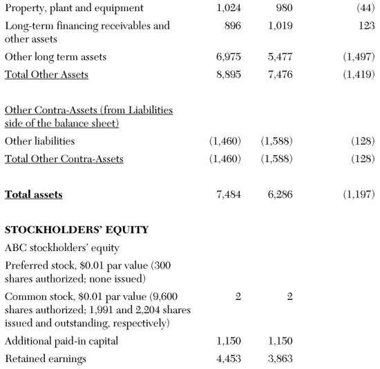
Note: All figures are in millions of dollars.

Figure 4.3 ABC Co.’s reorganized sources and uses of cash

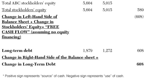
To calculate free cash flow, we simply add up changes in cash generated by assets and changes in cash generated by contra-assets. This number is part of free cash flow. We also need to add in the change in stockholders’ equity because the change in stockholders’ equity is the result of net income, which is also a potential source of cash. As shown in Figure 4.3, for ABC the free cash flow generated between 2012 and 2013 was –$608 million. Notably, this is the same amount as the change in long-term debt (also shown in Figure 4.3). Essentially, the flow in cash occurred from the right-hand side of the balance sheet, in the form of an increase in long-term debt of $608 million. This flow offset the decline in cash generated by adding the change in the left-hand side of the balance sheet and the change in shareholders’ equity.

With this approach, we can also see how changes in specific balance sheet accounts affect free cash flows. For example, suppose that we are running a manufacturing business and we consider a policy of increasing the amount of time we take to pay our suppliers. This would mean that our accounts payable would increase. The accounts payable is a short-term liability,⁸ and you learned in Chapter 2 that an increase in a liability generates cash. Therefore, this policy of taking longer to pay suppliers would result in an increase in sources of cash and no changes to uses of cash. (We are assuming that this policy has no additional effects on the business, such as our suppliers charging us more as a penalty.) So, the net result is that additional cash is created on the left-hand side of the balance sheet and flows to the right-hand side of the balance sheet for distribution to debt and equity holders in the firm. So, if all else remains the same, a policy of taking longer to pay our vendors will result in increased free cash flow.

Figure 4.4 Balance sheet simplified into a smaller set of macro accounts

Net working capital consists of short-term assets (such as accounts receivable and inventory) minus short-term liabilities (such as accounts payable and deferred taxes). An important item to remember is that for all the calculations presented so far involving free cash flows, short-term liabilities have been moved to the left-hand side of the balance sheet. In effect, this creates a contra account on the left-hand side of the balance sheet for short-term liabilities. The sum of the short-term assets account and the short-term liabilities contra account equals net working capital. Another important thing to note is that the cash account, which is part of short-term assets, contains only cash needed to run the business (that is, operating cash). It does not contain excess cash. We discuss in a moment where to place excess cash.

With the identification of these two macro accounts, we can now state a general formula for calculating free cash flows. Because we are interested in cash generated by the left-hand side of the balance sheet and available to the right-hand side, we will generate a sources/uses of cash. Basically, free cash flow is given by the following formula:

NWC refers to net working capital, LTA refers to long-term assets, and ∆ is a symbol denoting “change in.” Therefore, this formula states that free cash flow can be computed by simply measuring the negative of the change in net working capital minus the change in long-term assets as we go forward in time. Because net working capital and long-term assets are asset-side accounts, an increase in these accounts uses cash (rather than generates cash) and will therefore decrease free cash flow.

There is one item missing from Equation 2. That is the cash generated from running the business. The cash account in net working capital contains only the cash needed to run the business. It does not contain the cash that was generated from running the business. So, we need to include this into our free cash flow calculation. The following modified equation for free cash flow includes this cash generated by the business:

EBIAT refers to earnings before interest and after taxes. EBIAT is basically after-tax operating profits. One might wonder why we are using EBIAT rather than the traditional net income account to measure cash generated by the business. In fact, EBIAT and net income are quite close. The primary difference between the two is that net income includes interest paid on debt as an expense (along with the associated tax shield), whereas EBIAT is before interest so that it does not include any interest expense. To measure free cash flow, we want to exclude the right-hand side of the balance sheet, including any effects of capital structure decisions (decisions about the debt versus equity composition of the financing of the firm). Interest expense is a direct effect of capital structure policy. The more debt a firm uses, the higher its interest expense, and vice versa. Because we are only interested in cash generated from running the business (that is, the left-hand side of the balance sheet), we do not want to include interest expense in our measure of free cash flow. Therefore, we use EBIAT rather than net income. As a result, the free cash flow measure in Equation 3 is a measure of all cash that is generated by the left-hand side of the balance sheet and available for distribution to the financial claimants on the right-hand side of the balance sheet (in the form of interest, principal repayments, dividends, stock buybacks, and so on).

Because new working capital only contains cash needed to run the business, EBIAT fills in the missing piece in the free cash flow formula for cash thrown off from operating the business. Equation 3 states that free cash flow is simply equal to minus the changes (increases) in net working capital and long-term assets as a result of running the basic business and the cash generated from running this business.

We will make one more change to the free cash flow formula by defining long-term assets more clearly. Long-term assets are simply the long-term fixed assets, or net property, plant, and equipment (PPE) of the business. The net PPE account can be broken down into two accounts: gross PPE and accumulated depreciation. Gross PPE is simply the total amount spent on long-term fixed assets since the inception of the firm. The gross PPE account includes expenditures for both acquisition of new PPE and maintenance of existing PPE. Accumulated depreciation is an account that captures the total depreciation since the inception of the firm. Every time a depreciation expense is taken, that amount is added to the accumulated depreciation account. The net of gross PPE and accumulated depreciation is net PPE, which is effectively the firm’s current PPE level. The following equation summarizes our breakdown of the net PPE account:

We are using Accum Depr to denote accumulated depreciation. If long-term assets equals gross PPE minus accumulated depreciation, the change in long-term assets must be equal to the change in gross PPE minus the change in accumulated depreciation:

Of course, the change in gross PPE in a given period is simply equal to the capital expenditure for that period. Similarly, the change in accumulated depreciation is simply equal to the depreciation expense for that period. Therefore, we have

where CapEx denotes capital expenditure, and Depr denotes depreciation. We can now substitute this result into Equation 3:

This is our final free cash flow formula, and we will use it for the remainder of this book. This formula basically says that free cash flow during a specific period equals the cash generated by the business during that period minus any changes (increase) in net working capital during the period minus any capital expenditures during the period plus the depreciation expense taken during the period. This free cash flow is then available for distribution to all financial claimants on the right-hand side of the balance sheet.

The following example using the forecasted financial statements from Chapter 3 for ABC Co. illustrates how to use the free cash formula in Equation 7 to calculate free cash flows for a company. In Figure 4.5, we implement the free cash flow formula to forecast free cash flows for ABC from 2014 through 2018. In 2014, for example, our first step is to calculate earnings before interest and taxes (EBIT), which is simply total net revenue minus cost of goods sold (COGS) (which includes the cost of products, cost of services, and financing interest), research and development expenses (R&D), SG&A expenses, and other expenses. This produces an EBIT value of $887M for 2014. We then subtract taxes from this to produce the EBIAT value needed in the free cash flow formula. The tax rate used is the same as the tax rate projected in Figure 3.1, which is 21.24%. This calculation produces an EBIAT value of $699M for 2014. We then subtract out the changes in net working capital. Net working capital is computed for each year: $53M in 2014 and $48M in 2013 (not shown in Figure 4.5). Therefore, net working capital increased by $5M in 2014.

Figure 4.5 Financial Projections ($MM)

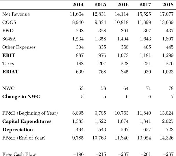
To finish calculating free cash flow for 2014, we need to determine capital expenditures and depreciation. The first thing we do to determine this is to determine property, plant, and equipment (PP&E) levels at the beginning of year (BoY) and at the end of year (EoY). In calculating PP&E, we will include the accounts Property, Plant, and Equipment, as well as long-term financing receivables, and other long-term assets. The beginning of year value for 2014 is simply the EoY value for 2013. This is $8,895M. The EoY value for 2014 is $9,785M. We can now determine capital expenditures and depreciation using the following equation, which has to hold each year:

This equation simply states that ending PP&E balance each year must be equal to the starting PP&E balance for that year plus any capital expenditures that were made that year (as these would add to the PP&E that a firm owns) minus any depreciation for that year (as these would reduce the value of PP&E that a firm owns). For 2014, we know two of the items in this equation already: PP&E (BoY) and PP&E (EoY). So, if we can determine one of the remaining quantities, the other one will be automatically determined by Equation 8. We will determine the depreciation amount for 2014 by maintaining the previous year’s depreciation level as a percentage of beginning of year PP&E. This turns out to be 415 / (980 + 1,019 + 5,477) = 5.55% for 2013. So, if we maintain this percentage for 2014, the forecasted depreciation expense will be 5.55% times beginning of year PP&E (1,024 + 896 + 6,975 = 8,895). This yields a 2014 depreciation amount of 5.55% × 8895 = 494. Then, from Equation 8, the capital expenditures can be determined as 9785 + 494 – 8,895 = 1,383. Thus, we now have determined all the components needed to calculate the free cash flow formula. For 2014, this turns out to be –$196M. As a result, our plug accounts, long-term debt, and other long-term liabilities⁹ must increase by $196M in 2014 to produce the needed cash for the left-hand side of the balance sheet.

The free cash flow calculations for the years from 2015 through 2018 in Figure 4.5 follow a similar approach. We will use the cash flows in this example in later chapters as we develop our overall valuation framework.

We will develop another example to demonstrate how to value a project. Let’s analyze the following project in which ABC Co. is considering investing. The project is a new product introduction. The new product will require an initial investment of $20M per year for two years to develop a new manufacturing facility. This facility would be depreciated straight-line to a zero salvage value over five years. After the manufacturing plant is built, sales would begin (in Year 3 of the project). However, in preparation for new sales, an investment would need to be made during the second year to build up a parts inventory and cash needed for short-term needs. This investment would be equal to 25% of expected sales in the following year, and this investment would need to remain in place at 25% of expected next-year sales throughout the life of the product. The new product is expected to generate sales of $71.4M in the first year that it is introduced, $82.8M in its second year, $43.4M in its third and fourth years, and $21.6M in its fifth and final year, after which the product would be dropped as it would become obsolete. The gross margins for the product (which include the depreciation expense) are expected to be 29% each year there are sales. Other costs for running this new business would be 10% of sales. The marginal tax rate for the ABC is 25%.

Figure 4.6 contains the free cash flows for this project. For the first two years, we are investing $20M each year to build a manufacturing plant. These investments get captured as capital expenditures (CapEx). Once the plant is built, the total $40M investment is depreciated over a five-year period ($8M per year), which results in a depreciation expense of $8M per year. Because there are no sales or investment in net working capital in 2014, applying Equation 7 gives a free cash flow (FCF) of –$20M for 2014. Because sales are expected to be $71.4M in the first year, net working capital of $71.4M × 25% = $17.85M must be in place.¹⁰ Therefore, the NWC balance at the end of 2015 (beginning of 2016) is $17.85M. Thus, there is an increase in NWC in 2015 of $17.85M (as NWC was zero in the prior year). So, applying Equation 7 gives a total free cash flow of –$37.85M for 2015. The first year of sales is 2016. Sales are $71.4M. Due to the 29% gross margin, the cost of goods sold (COGS) is $71.4M × (1 – 29%) = $50.69M. Selling, general, and administrative (SG&A) expenses are 10% of sales: $71.4M × 10% = $7.14M. Therefore EBIT for 2016 is $13.57M, and EBIAT at a 25% tax rate is $10.18M. There is no further CapEx because the plant is now fully built; however, the plant begins depreciating and so there is a depreciation expense of $8M. Applying Equation 7 gives a free cash flow amount of $15.33M for 2016. The calculations for future years follow in a similar manner. The question of whether to undertake this project requires us to determine how much value is created (or destroyed) if ABC Co. undertakes the project. We will continue this example and do this valuation in Chapter 6, “Putting It All Together: Valuation Frameworks.”

Figure 4.6 Financial Projections ($000s)

If we want to calculate free cash flow, rather than starting with the balance sheet as we did in the previous section, we could instead start with the income statement. In other words, to calculate free cash flow, we start with the business and how much cash the operations throw off. This, of course, is given by net income. However, we need to recognize just as we did before that free cash flow is really about how much cash is generated by the business independent of capital structure decisions. So, we want to exclude interest expense. This leads us to EBIAT, just as in the previous section.

Another item to note about net income is that there may be noncash expenses in the income statement. The most common one is depreciation, so we will represent all noncash charges with this term. Because depreciation is really a noncash charge, it really should not affect free cash flow. However, because depreciation is not excluded from the income statement, we need take it out and create a new operating cash flow result called EBIDAT (earnings before interest, depreciation, and after taxes). This could be our starting point for calculating free cash flows. However, this leaves another minor problem. Even though depreciation is a noncash charge and should not be included in free cash flows, it does provide the company a tax shield, which is an actual cash saving. The IRS allows firms to deduct depreciation as an expense in the calculation of their taxes. This depreciation expense thus lowers the company’s tax bill, which is a real cash saving for the firm. Therefore, we cannot fully take out the depreciation expense in EBIDAT. A portion of it (the tax savings) needs to remain in the free cash flow formula. This is solved in the following common way. We start the free cash flow calculation with EBIAT, just as we did before. Because EBIAT contains depreciation as an expense, it contains the depreciation tax shield.

However, because the depreciation expense itself should not be included in the free cash flow calculation, we add back the depreciation as a separate step. We therefore have the result

To calculate free cash flow, we now just need to include the effect of operations on the asset side accounts, which are net working capital and net PPE. Specifically, we want the cash effects to these two accounts. Therefore, we want to subtract out any increase in net working capital, and we want to subtract any capital expenditures. This leads to the same result that we calculated in the previous section:

This provides another perspective on the formula for calculating free cash flows, which is more income statement centric rather than the balance sheet centric approach used in the previous section. Both approaches are quite similar, and both of course lead to the same final free cash flow formula.

2. The final part of this process is to then make sure that this amount and form of financing are in place (i.e., to execute the amount and form of financing). We talk more about this later in the book.

3. Note that this is not the same as the accounting definition of cash flow that we discussed in Chapter 2. The accounting definition of free cash flow, for example, incorporates the effects of financing into its definition of cash flow. Free cash flow, however, does not incorporate financing effects because it is largely driven by the left-hand side of the balance sheet. For this reason, free cash flow is sometimes referred to as operating cash flow to clearly distinguish it from the accounting definition of cash flow.

4. As mentioned previously, this view changes for financial institutions. In a financial institution, both the left-hand and right-hand sides of the balance sheet contain the operating activities.

5. It is important to note that by debt, we specifically refer to long-term debt. Short-term liabilities such as accounts payable or notes payable that typically are categorized as part of working capital are moved to the left-hand side of the balance sheet. On the left-hand side, they show up as contra accounts and are netted against short-term assets such as inventory and accounts receivable. We then net these short-term assets and the contra accounts representing the short-term liabilities to form an asset-side account called net working capital. So whenever we refer to a balance sheet as having net working capital, it automatically indicates that the liability-side of the balance sheet only contains long-term liabilities.

6. As discussed in Chapter 3, future operating activity targets automatically imply a certain set of balances in all the accounts on the left-hand side of the balance sheet.

7. This is why accountants usually refer to a cash flow statement as reconciling to the cash account.

8. Again, note that even though this item is a liability, we are considering it a left-hand side account; i.e., it is a contra asset account.

9. Note that we are using a slightly different interpretation of other long-term liabilities here than was used earlier in Figure 4.3 with regard to the sources and uses of cash. Here, we are treating other long-term liabilities as a potential financing vehicle (like long-term debt), whereas we had treated this as a contra-long-term asset account earlier. An example of a long-term financing vehicle might be hybrid securities such as convertible notes.

10. As sales increase, the working capital will need to increase, and there will be further investments into working capital, which in turn will create negative cash flow. However, as sales decrease in later years, the working capital amount can be reduced, thus creating positive cash flow as the firm takes back working capital from the project.