6. Putting It All Together: Valuation Frameworks

where E(CF₁), E(CF₂), and so on are expected future cash flows, r denotes a discount rate, and Value₀ is the value of the project that we are trying to measure. In the previous chapters, we discussed how to calculate the cash flows and the discount rates. Each year we construct projected financial statements for the project or firm that we are interested in valuing. From these financial projections we then calculate free cash flows:

The free cash flows from this equation are used as the expected future cash flows in Equation 1.

The discount rate is calculated by determining the riskiness of the free cash flows. The discount rate under each cash flow compensates for the riskiness of that cash flow. Because free cash flows are coming from the left side of the balance sheet of the asset we are trying to value, the discount rate is simply the asset cost of capital. To determine the asset cost of capital, we need to use a combination of comparable assets, the CAPM

and the asset cost of capital formula:

We have two final concepts to discuss to have a fully developed valuation methodology. The first is how to deal with the effects of debt financing, specifically the tax shield. The second is how to compute the sum of an infinite number of cash flows as we apply Equation 1.

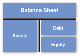
Figure 6.1 depicts the balance sheet view of the asset we are trying to value. The presence of debt on the right side of the balance sheet and the fact that the interest on debt is tax deductible imply that a tax shield is created on the left side of the balance sheet. From Equation 2, the free cash flows that we calculate for the asset are independent of the capital structure and therefore do not capture the value of this tax shield. So, we must incorporate the value of the tax shield in another way. In this section, we present three valuation approaches for executing Equation 1. The valuation approaches differ primarily in how this tax shield is incorporated. The adjusted present value (APV) approach treats this tax shield as a separate asset and calculates its value by applying Equation 1 a second time—this time to value the tax shield. The weighted average cost of capital (WACC) approach incorporates the tax shield benefit into the discount rate. The flow to equity (FTE) approach utilizes cash flows to equity rather than free cash flows. Therefore, it deducts the interest payment in the process of calculating cash flows, thus incorporating the tax shield value in the cash flows.

The second issue that we have is how to deal with potentially an infinite number of terms in Equation 1. For some assets, the cash flows will be expected to cease after a finite number of years. In these cases, we would simply apply Equation 1 out to the number of years until the cash flows end. However, many assets, such as a firm, will have expected cash flows out to perpetuity. In these cases, we have an infinite number of cash flows and, therefore, an infinite number of terms in computing Equation 1. The general approach for dealing with this situation is to truncate Equation 1 at some point and have a final term, a terminal value, that captures the remaining infinite number of cash flow terms. This section introduces several techniques to calculate this terminal value.

The present value of operating assets is calculated by discounting the free cash flows that these assets generate. Because it is the assets that generate these free cash flows, the discount rate that appropriately compensates for the riskiness of the free cash flows is the cost of assets, R_A.¹

In the numerators, we have dropped the expectation term, but it should be understood that all of the free cash flows occur in the future, and therefore, FCF₁, FCF₂, ... are all expected free cash flows.

We can similarly restate the calculation of the tax shield present value. Suppose that the amount of debt on the balance sheet in future periods is denoted as D1, D2, .... The interest rate on this debt is given by R_D. Therefore, in year n, there is an expected interest payment of D_n × R_D. Because this interest payment is tax deductible, the tax authorities effectively subsidize this payment by an amount equal to the tax rate, τ, multiplied by the interest payment. Therefore, the tax shield generated in year n would be τ D_nR_D. With this result, we can now state the general formula for the APV of an asset:

As an example of the tax shield calculation, suppose that we have a project that we are trying to value with a fixed level of debt, D. Therefore, the level of debt is expected to remain at the level D forever. We will calculate the present value of the tax shield in this case:

It is easy to show mathematically that

Therefore, we have the result that in the case of a fixed level of debt D into perpetuity with a tax rate of τ

We show examples of how to utilize the APV approach shortly.

The term TV in the numerator of the last free cash flow term denotes the terminal value of the asset at the end of n years. In this section, we present three alternative methods for computing this terminal value: the liquidation value, the growing perpetuity value, and the multiples value.

We will now demonstrate how to use the APV approach with the terminal value calculated by using the liquidation value approach. Consider the project in which ABC Co. was thinking about investing, described at the end of Chapter 4, “Free Cash Flows.” The free cash flows for this project were calculated at the end of Chapter 4 in Figure 4.6. We will value this project, a new product introduction, to determine whether ABC Co. should undertake this project.

Figure 6.2 shows the results of applying the APV approach to this project. The current time is at the end of 2013. We assume that we have checked comparables and gone through the cost of capital calculation process described in the previous chapter to arrive at an asset cost of capital for the project of 11%.³ After determining free cash flows (FCF), a terminal value (TV) is calculated in 2020. It is assumed that the manufacturing plant that was built for the project in 2014 and 2015 can be sold at the end of 2020 for $5M. However, because the plant has been depreciated down to zero book value, this sale represents a gain and ABC Co. would have to pay tax at ABC’s marginal corporate tax rate (25%) on this gain. Therefore, the liquidation value is $5M × (1 – 25%) = $3.75M. The free cash flows and terminal value are added together and discounted at the 11% asset cost of capital rate to produce a present value (PV[FCF + TV]) for each year.

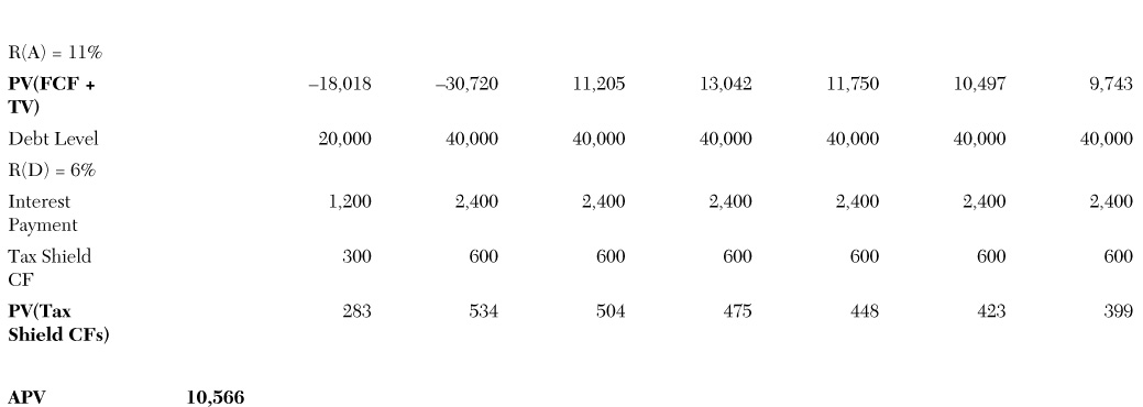
In the APV approach, the tax shield value of the project must now be calculated. We assume that the $20M investments in 2014 and 2015 to build the manufacturing facility are financed by debt. Therefore, the debt level for the project is at $20M at the end of 2014, and $40M at the end of 2015 and onward. We assume a cost of debt (R[D]) of 6%. This leads to interest payments of $1.2M in 2014 and $2.4M in 2015 and beyond. These interest payments produce a yearly tax shield of the interest payment times the tax rate (25%). The present value of each of these tax shields is computed by discounting at the cost of debt of 6%.

The sum of the present values of the free cash flows, terminal value, and the tax shield cash flows produces an APV of $16.4M. Therefore, by investing in this project, ABC Co. would derive $16.4M of net positive value (which would accrue to its equity holders).

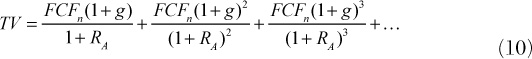
In this equation, the free cash flows have settled down to a smooth growth rate of g. Because the free cash flows are growing at a constant rate g, we can solve for the terminal value in closed form. We first multiply both sides of this equation by (1 + g) / (1 + R_A):

We then subtract this equation from the first one. Because all of the terms on the right side of Equation 11 are present on the right side of Equation 10, this subtraction leaves us with a much simpler equation:

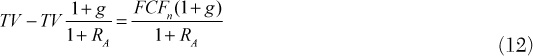
We can now solve this equation for TV on the left side:

This expression can be simplified to

Equation 14 provides a simple formula for calculating a terminal value once the cash flows have settled to a growing perpetuity. As a result, this formula is known as the growing perpetuity formula, and the terminal value is known as the growing perpetuity value.

A special case of this formula is the situation when the free cash flows are not growing, so that the free cash flows go on forever at a fixed level (i.e., a perpetuity). In this case, g = 0, so that the formula simply becomes the following perpetuity formula for terminal value:

It is important to note here that for the growing perpetuity formula to work, the growth rate of the free cash flows, g, must be less than the asset cost of capital, R_A.⁴ We demonstrate how to implement APV with the growing perpetuity approach for calculating a terminal value by valuing ABC Co. today (end of 2013). The free cash flows for ABC were calculated at the end of Chapter 4 in Figure 4.5. In Figure 6.3, we calculate the enterprise value⁵ and equity value of ABC utilizing APV. We first make one small change to the cash flows from Figure 4.5. In Figure 4.5 we determined ABC Co.’s free cash flows to be negative every year. This is primarily because of ABC’s large amount of capital expenditures; they are currently investing heavily in their businesses to grow them. Of course, to survive, ABC has to produce positive free cash flows in the long run. We accelerate this process and assume that in Figure 6.3 the heavy capital expenditures are finished and that the only ongoing capital expenditures are simply to maintain the business at a normal growth rate. Thus, capital expenditures are reduced, and the resulting free cash flows (FCF) in 2015 and beyond are now positive.

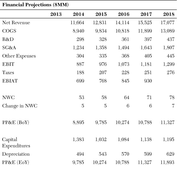
Once the free cash flows have been calculated, a terminal value needs to be determined. We calculate a terminal value (TV) at the end of 2018 using the growing perpetuity formula, Equation 14. We assume an asset cost of capital of 9% has been derived⁶ and that a perpetual growth rate of 4% has been determined. The growth rate assumption is an important one. Because this growth is expected to occur forever, we must be careful not to use too high of a growth rate; otherwise, our calculations would be assuming that ABC would grow faster than the world economy forever (which would implicitly assume that ABC would eventually become the world economy). Historically, the world economy has had a real growth rate of about 1.5%. Long-run inflation for the world historically has been about 2.5%. Therefore, the historical long-run nominal growth rate of the world economy has been about 4%, which is the number we use for the growth rate in Equation 14. The terminal value is therefore

We can now calculate the present value each year for the sum of the cash flow and terminal value each year.

To finish the APV calculation, we now need to calculate the present value of the tax shields. The debt levels (Debt Level) are calculated from Figure 3.1.1 (which contains the pro forma financials for ABC) as the sum of long-term debt and long-term liabilities. The cost of debt is assumed to be 6%. The product of the debt level each year and the interest rate produces the interest payment for each year. The tax shield for each year (Tax Shield CF) is simply the product of the interest payment and the corporate tax rate (21.24% from Figure 3.1.1). Because the tax shield cash flows go on forever, we need to calculate a terminal value in 2018 for the tax shields as well. We do this by assuming that the debt level stays fixed at the 2018 level forever; therefore, we can use the perpetuity formula with no growth, Equation 15. This produces a terminal value of $61M / 6% = $1,022M. We can now calculate the present value each year for the sum of the tax shield cash flow and terminal value each year.

The APV (Enterprise Value) is simply the sum of the present values of the free cash flows and terminal value and the present values of the tax shields and tax shield terminal value. This is equal to $7,928M for ABC. To calculate the equity value, we just need to subtract the current debt value from the enterprise value. The current debt value (end of 2013) from Figure 3.1.1 is the sum of the long-term debt and other long-term liabilities, which equals $3,339M. Therefore, the equity value for ABC is $7,928M – $3,339M = $4,589M.

The multiples approach is a common way to calculate a terminal value. The concept behind this approach is to calculate a terminal value by simply computing a market value for the asset side of the balance sheet at the terminal value point. This market value is determined by looking at the market values of comparable assets today and proportionately impute a similar valuation for the terminal value of the asset we are trying to value. We do this by assuming that the asset we are valuing will have a terminal value multiple that is equal to that of the multiples of the comparables.

It is easiest to understand this approach through an example. Figure 6.4 contains the valuation of ABC that we did previously in Figure 6.3. The APV process and the numbers are the same. In Figure 6.4, however, we assume that the terminal value of free cash flows (TV) is calculated as a multiple rather than as a growing perpetuity. To calculate this terminal value, therefore, we need to determine what the appropriate multiple should be. Figure 6.5 contains a table of comparable firms and their enterprise value multiples based on current (2013) market values. For example, the EBIT multiple of 6.4 for DEF Corp. indicates that DEF’s current enterprise value is 6.4 times the EBIT it produced for the previous year. Similarly, the EBITDA multiple indicates the ratio of enterprise value to EBITDA.⁷ The B/M multiple is referred to as a book-to-market multiple, and it denotes the ratio of the book value of assets to the market value of assets (enterprise value). We will use an EBIT multiple to calculate the terminal value for ABC in Figure 6.4. Because all the firms listed in Figure 6.5 are comparables to ABC, we will simply use their average EBIT multiple, 7.8, and assume that it applies to ABC in 2018. So, we can now calculate the terminal value for ABC in 2018 as 7.8 times ABC’s 2018 EBIT, which is calculated earlier in Figure 6.4 as $1,299M. Therefore, the terminal value is 7.8 × $1, 299M = $10,130M.

To finish the APV calculation, we need to determine the tax shield value. This is done in exactly the same way and using the same numbers as in Figure 6.3. The only difference is that a terminal value of tax shield cash flows does not need to be included. This is because we have already captured this in the terminal value of free cash flows. The multiples of comparable firms in Figure 6.5 use market values, which naturally include all tax shields. So, for example, DEF’s EBIT multiple is the ratio of DEF’s enterprise value to EBIT where the enterprise value is the total asset value of DEF including the tax shield value. Therefore, when we applied an EBIT multiple to calculate ABC’s free cash flow terminal value, we also captured the tax shield terminal value. So, we do not need to do a separate tax shield terminal value.

The resulting enterprise value for ABC using the multiples approach is $7,673M and ABC’s equity value is $4,334M.

The obvious drawback with the multiples approach is that it assumes that the multiples that are present in the marketplace today will apply in the future at the point in time we truncate the free cash flow calculation and do a terminal value. This assumption needs to be checked by looking at the historical stability of the multiples that are being used for the terminal value calculation. The greater the historical variability of multiples, the greater the error that will be likely in the terminal value. So, one should choose the multiples that have been the most stable, and these usually vary from industry to industry.

For example, if we are valuing a firm, we might typically expect the firm to maintain a certain debt ratio through time rather than a certain debt level (or schedule of debt). The application of the APV concept would separate the valuation of the free cash flows and the valuation of the tax shield. The valuation of the tax shield assumes a debt schedule of some kind so that one knows how much debt is expected to be on the balance sheet in the future. With this future level of debt and the associated cost of debt, an interest tax shield can be computed each year. However, with a fixed debt ratio policy, the amount of debt in the future is unknown. This is because the debt level in the future is tied to the asset value in the future (because the debt level is proportional to the asset value when a fixed debt ratio policy is followed). Of course, the asset value in the future is unknown. We do not know the value of the asset today (hence the reason we are doing a valuation), so certainly we will not know the value of the asset any point in the future either. Thus, if the asset value in the future is not known, we will not know the debt level in the future either; therefore, we will not be able to calculate the tax shield value with the traditional APV approach.

We solve this problem by incorporating the tax shield value calculation directly into the free cash flow valuation step. We do this by integrating the tax shield value directly into the discount rate used to value the free cash flows. This modified discount rate is called the weighted average cost of capital, or WACC. With the use of WACC, the APV approach can be implemented in one calculation rather than the two separate calculations that is normally required. However, it is important to note that the use of WACC is only appropriate when the asset to be valued has a capital structure policy where a fixed debt ratio will be used. In all other situations, the traditional APV approach must be utilized.

We will derive the WACC approach⁹ through the following simple scenario. Consider the APV approach in the case of a project lasting a single year. The value of this project is given by

This equation states the usual APV approach. The second term in this equation is the tax shield value, which comes from the $D of debt on the right side of the balance sheet of this project. The tax rate is given by τ. Notice that the discount rate associated with the tax shield is not R_D. This is because we have not specified a capital structure policy yet. Once we specify the capital structure policy, we will be able to determine this discount rate.

Suppose that the financial policy that is implemented for this project is one that keeps its debt ratio fixed at a constant level d permanently. In this case, , where A is the usual asset value. Rearranging this expression, we have that

We can now substitute for D into the earlier APV equation:

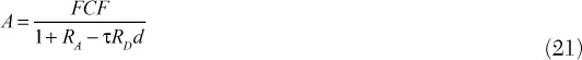
With the capital structure policy known, we can now figure out what the discount rate for the tax shield should be. The tax shield cash flow is given by τ R_DdA. Assuming that the tax rate, the cost of debt capital, and the capital structure policy are fixed, the only quantity that can vary (and thereby create risk) is A. Therefore, the discount rate that appropriately reflects this risk is R_A. So, the full APV formula is given by

Because APV is simply the value of the left side of the balance sheet, we can simply replace APV with asset value, or A:

We will now solve this equation for A:

We will eliminate R_A in this equation by using the asset cost of capital formula derived in the previous chapter

where E denotes equity value. Substituting for R_A in Equation 21 yields

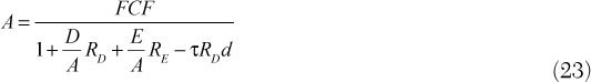
We can replace the term d with :

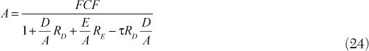
Rearranging the denominator then gives us a final formula for calculating A, or the APV:

Notice that the expression is very similar to the formula for the asset cost of capital. However, it has an extra (1 – τ) in it multiplying the cost of debt. This expression is commonly known as the weighted average cost of capital, or WACC.

What differentiates WACC from R_A is that WACC includes the tax shield into the discount rate by reducing the cost of debt. We can now rewrite Equation 25 as simply

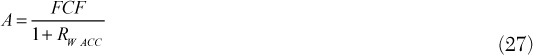
The use of WACC has effectively eliminated the two-step calculation process typically used in APV and replaced it with a one-step process where the discount rate on the free cash flows is WACC rather than R_A. Therefore, the WACC-based approach is simpler to implement and at the same time eliminates the difficulty discussed earlier of calculating APV in a situation where the debt ratio is held constant.

For simplicity, we have done this calculation for a one-year project (with only one free cash flow and one tax shield cash flow). However, it is easy to show that this derivation can also be done for multiyear projects as well. Therefore, we have the following general formula for valuing assets when a fixed debt ratio policy is in place:

Again, keep in mind that the WACC-based approach is simply a special case of the general APV approach. It can only be used in situations where one wants to calculate an APV and the asset being valued has a capital structure policy where a constant debt ratio is maintained.

We now demonstrate the WACC-based valuation approach by valuing ABC Co. again. This is done in Figure 6.6.

Figure 6.6 contains the same free cash flows as Figure 6.3, where we valued ABC Co. using APV with a growing perpetuity terminal value. However, we now assume a more realistic debt policy. In Figure 6.3, we assumed that the debt level was fixed at $4,812M from 2018 onward. Now in Figure 6.6, we assume that ABC Co. always maintains a fixed debt ratio. So, we can simply use WACC to calculate ABC’s enterprise value. A WACC of 8.5% is assumed for ABC. The terminal value of free cash flows is calculated using the growing perpetuity formula where we use WACC in place of R_A:

We assume the same growth rate as used in Figure 6.3: 4%. Thus, we arrive at a terminal value of $10,387M. We then calculate the present value of each of the free cash flows and terminal value by discounting at the WACC. The sum of these present values is ABC’s enterprise value, $7,791M. No separate calculation for determining tax shield value needs to be done because it is already incorporated in the WACC. ABC’s resulting equity value is $4,452M.

When we are valuing a company or a project, we are usually really after the value of the equity component of the project. With APV and WACC, we determine this equity value by first determining the value of the asset (because free cash flows are cash flows flowing from the asset to both debt and equity) and then subtracting out the debt value that is used to finance the company or project. FTE instead determines the value of equity directly by looking at just the cash flow to equity (rather than to both equity and debt). Therefore, all cash flows to debt holders are netted out of free cash flows each year to determine the cash flow to equity holders. Figure 6.7 provides a depiction of the cash flow to equity. Because the cash flows to debt are subtracted out, the resulting cash flows are quite different from free cash flows.

To determine the cash flow to equity holders, we need to modify the free cash flow formula we have developed. The free cash flow formula is

To get to cash flows to equity holders, we need to subtract out all flows to debt holders. There are two types of flows to debt holders: interest and principal. We will subtract out interest by modifying EBIAT to reflect earnings with interest taken out. This would be earnings after taxes, or simply net income. Therefore, instead of EBIAT, we would use net income. The second change to the free cash flow formula is to net out any principal payments. Principal payments on debt decrease the cash available for distribution to equity holders. This is why principal payments need to be subtracted out to arrive at the cash flow to equity holders. These two changes would result in the following cash flow formula:

NI denotes net income, and ∆Debt denotes the increase in debt level.¹⁰

The final question we need to answer is what is the appropriate discount rate. The value of equity is determined entirely by cash flows to equity because these are the only cash flows equity holders receive. In fact, using the present value relation, Equation 1, we can write down the value of equity today (time 0) as the discounted value of cash flows to equity:

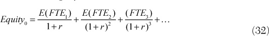
Therefore, the riskiness of equity comes entirely from the riskiness of FTE. So, the riskiness of FTE must be equal to the riskiness of equity. If this is the case, then the appropriate cost of capital to discount FTE must be the equity cost of capital. So, we have

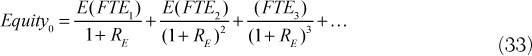
When we apply the FTE approach, we do not need to calculate a separate tax shield cash flow because the tax shield is already embedded in net income (NI). The only complication we need to worry about is a terminal value calculation, but we can do this using a growing perpetuity approach. We demonstrate the FTE approach in Figure 6.8 by valuing ABC Co. again, but utilizing the FTE approach.

Notice that in the upper part of this figure, we have net income now instead of EBIAT. To calculate net income, we have subtracted out the interest payment on debt. In the lower part of Figure 6.8, we have the debt level for each year (which comes from the projections in Figure 3.1.1). We calculate the interest expense by assuming a cost of debt capital of 6% and multiplying this by the debt level. For example in 2014, the interest expense is 3,584 × 6% = 215. From the NI value, we subtract out the changes in net working capital and capital expenditures, and add back depreciation to arrive at a number sometimes referred to as capital cash flows (CCF). From CCF, we subtract out the change in debt level for that year to arrive at the flow to equity.¹¹ We now need to calculate a terminal value in 2018. We do this using the growing perpetuity formula for FTE:

The cost of equity is assumed to be 14%, and we use the standard growth rate of 4%. This gives a terminal value of $5,939M. We now present value each of the equity cash flows and the terminal value at the cost of equity. Summing these present values then produces the value of ABC Co.’s equity, $4,680M. As discussed earlier, there was no need to do a separate tax shield cash flow because it was already captured in the net income.

A = OA + TS

However, recall from the previous chapter that our working assumption is that the tax shield value is substantially smaller than the value of the operating assets. In this case the total asset value, A, is approximately equal to the operating asset value, OA:

A = OA + TS

≈ OA

We can follow a similar logic with the cost of assets:

If the tax shield value is small relative to the value of operating assets, the operating asset cost of capital is approximately equal to the asset cost of capital.

2. There is no rule as to what point in time this truncation should occur. One rule that is used when changing or restructuring an asset is to work out the detailed cash flows until the changes have all been fully implemented. Another common rule is to truncate when one loses visibility on (or loses sufficient confidence in the accuracy of) forecasted future financial statements.

3. It is important to note that the cost of capital for the project is not the same as the cost of capital for ABC Co. If the project has a risk profile that differs from ABC, the cost of capital has to be calculated using comparables similar to the project rather than to ABC.

4. Otherwise, the rate of free cash flow growth is so high that it causes the terminal value to have infinite value.

5. Enterprise value is another way of referring to the asset value of the firm.

6. We assume that this calculation was done using the techniques described in Chapter 5, “Cost of Capital.”

7. EBITDA refers to earnings before interest, taxes, depreciation, and amortization. EBITDA is similar to EBIT, but it tries to strip out all noncash expenses as well. Therefore, EBITDA is sometimes used as a measure of operating cash flow.

8. Note that the debt level may be fixed or there could be a debt schedule (where the debt level either increases or decreases in a predetermined manner).

9. Although we treat this approach as one that is distinct from APV, note that this is not really the case. The WACC approach is really a subset of the APV approach. It is a quick (one-step) way to implement APV when the capital structure policy is stipulated to maintain a fixed debt ratio. Therefore, it is more correct to refer to the WACC approach as a WACC-based APV approach.

10. Principal repayments would result in a negative value for ∆Debt, so the application of this formula would result in principal repayments decreasing cash flows to equity, as we expect.

11. In Figure 6.8, the 2013 debt level is $3,339M, which comes from Figure 3.1.1.