
3. Traditional Valuation Methods
Market View
In April 2012, Cristina Fernández de Krichner, Argentina’s president, announced that the government was seizing control of 51 percent of YPF, the country’s largest hydrocarbon producer. The action would be executed by expropriating shares from Repsol, the Spanish oil and gas company, reducing its stake in YPF from 57.4 percent to 6.4 percent. The Argentinian president justified the nationalization by citing both Repsol’s underinvestment in YPF and YPF’s excessive dividend payments to Repsol.
YPF accounted for approximately 45 percent of Argentina’s hydrocarbon production and had generated $1.3 billion in net income in 2011. Argentina had spent $9.4 billion on fuel imports in 2011 and did not expect national production to be sufficient in 2012 either. The government was facing a cash crunch and was unable to raise debt. Following its default in 2001 and the ongoing legal battles with global creditors, Argentina had been shut out from the international debt market for nearly a decade. The nationalization of YPF was viewed as an opportunity to gain access to the company’s hydrocarbon production and resulting cash flows.
YPF was privatized in 1993. In 1999, Repsol purchased a 98.7 percent stake in the company for $13.2 billion. Between 1999 and 2011, Repsol sold part of its investment in YPF, but by April 2012, it still owned a majority stake of 57.4 percent. According to Repsol’s consolidated financial statements at year end 2011, the book value of the 57.4 percent stake in YPF was worth €4.1 billion. The Argentinian subsidiary accounted for approximately 62 percent of Repsol’s production, 47 percent of proved reserves, 20 percent of revenue, 26 percent of operating income, and 21 percent of net income.
In May 2012, Repsol announced that it was filing for international arbitration before the World Bank’s International Centre for Settlement of Investment Disputes (ICSID) and would seek compensation in the amount of $10.5 billion. The financial community had little hope regarding the outcome of the arbitration, though; the Argentinian government had already announced that it would not pay any restitution. In the three months following the expropriation, Repsol’s stock price fell by approximately 40 percent. YPF had to be deconsolidated, wiping €4.7 billion from Repsol’s balance sheet and €38.0 million from its income statement. The expropriation also cost Repsol its investment-grade credit rating. The three largest credit rating agencies (Standard & Poor’s, Moody’s Investors Service, and Fitch Ratings) expressed concerns regarding Repsol’s ability to deliver the growth, earnings, and cash flows it had forecast without YPF; as a consequence, they all downgraded Repsol’s debt.
Although cases of expropriation of this magnitude are rare, many companies that make cross-border investments must take into account additional risks, including country/political risk and expropriation risk.
A survey by Bancel and Mittoo (2012) shows that the vast majority of valuation experts rely on two time-tested approaches to valuation: the free cash flow (FCF) to the firm model, used by 87 percent of respondents, and earnings multiples, used by 76 percent of respondents. However, a variety of alternative valuation methods exist. An earlier survey by Graham and Harvey (2001) showed that when chief financial officers (CFOs) make capital budgeting decisions, they prefer discounted cash flow (DCF) models and earnings multiples, but they also use alternative valuation methods. For example, real option analysis and the adjusted present value (APV) model are always or almost always used by 27 percent and 11 percent of respondents, respectively. Nonetheless, no valuation method is as widely used as the FCF to the firm model and earnings multiples to value a company in the context of mergers and acquisitions (M&As).
This chapter focuses on these two widely used valuation methods and addresses the following key questions:
• What are adjusted earnings multiples, and how can they be used to value a company?
• How can the FCF to the firm model be effectively implemented?
• How are the FCFs calculated?
• How is the weighted average cost of capital calculated?
• How can the continuing value of a target be estimated?
1 Earnings Multiples
One of the most common approaches to valuation involves the price-to-earnings (P/E) ratio. For example, brokerage firms frequently advise their clients to buy (or sell) a stock if its P/E ratio falls below (or rises above) some normal trading range, suggesting some form of market mispricing. This type of ad hoc valuation is typical of the small share-block market segment, but it also has proponents in the large share-block market segment, or market for corporate control. (We distinguish between the market for corporate control and the small share-block market because the cost of obtaining majority control of a company almost always necessitates paying a premium above the company’s market value, as discussed in Chapter 1, “Valuation: An Overview.”)
Earnings multiples can be calculated for a variety of earnings-based metrics. The most widely used ones are based on earnings after taxes (P/E), earnings before interest and taxes (P/EBIT), and earnings before interest, taxes, depreciation, and amortization (P/EBITDA). Regardless of which multiple is used, “earnings” should be defined with reference to a company’s permanent earnings—that is, its recurring operating earnings, excluding such one-time items as discontinued operations, extraordinary items, and one-time write-offs and charges; Chapter 5, “Accounting Dilemmas in Valuation Analysis,” shows how to calculate permanent earnings. The choice of an earnings multiple can vary among industries and analysts; however, when an analyst is using both earnings multiples and a DCF model, the P/EBITDA ratio appears to be the metric of choice because of its proximity to a company’s operating cash flow.
Earnings multiples can also be calculated for a variety of time periods. A trailing multiple, on the one hand, is obtained by dividing the current closing market price per share by the historical earnings per share (EPS) reported for the most recently completed accounting period (quarter or fiscal year). A forward multiple, on the other hand, is the current closing market price per share divided by forecast EPS. Forecasted EPS figures can be obtained from data vendors such as Thomson Reuters and Zacks Investment Research. Forward multiples are sometimes adjusted upward or downward to reflect changes in market sentiment or for information that is expected to affect a company’s share price (for example, additional earnings growth associated with the announcement of a new product launch or a new business acquisition).1
Regardless of the particular earnings multiple chosen, it is important to remember that such multiples are only relative measures of value. As Chapter 1 points out, P/E ratios vary greatly among industries.
Earnings multiples are frequently used in the context of M&As to provide an estimate of a target’s value. The principal reason they are popular is that they avoid the time-consuming process of modeling a target’s operations. When using earnings multiples, analysts perform either a comparable company analysis or a comparable transaction analysis. Both analyses require identifying a benchmark that serves as a basis for estimating the target’s value. Under the comparable company analysis, the benchmark is a group of comparable companies—that is, companies that are similar to the target in terms of business (such as products, markets, and business model) and risk characteristics. These companies are often competitors of the target. Under the comparable transaction analysis, the benchmark is a set of comparable transactions—that is, acquisitions that are similar to the acquisition under review. These transactions usually have taken place in the last three to five years in the target’s industry and might have involved some of the target’s competitors. Whether an analyst performs a comparable company analysis or a comparable transaction analysis, the steps to implement the earnings multiple approach and determine a target’s value are the same:
1. Identify the group of comparable companies or the set of comparable transactions that will serve as the benchmark.
2. Collect the earnings multiple (such as the P/E ratio) for each comparable company or transaction.
3. Calculate the average earnings multiple for the group of comparable companies or the set of comparable transactions.
4. Multiply the average earnings multiple (step 3) by a target’s earnings to obtain an estimate of its price. This price is often called the implied price because it is implied from using a model. The implied price can then be compared to a target’s market price per share (stock price). The target appears fairly valued if its stock price is equal to the implied price, undervalued if its stock price is lower than the implied price, and overvalued if its stock price is higher than the implied price.
To illustrate the use of earnings multiples, we return to Mattel. We perform a comparable company analysis using P/E ratios.
Steps 1 and 2
No toy manufacturer has exactly the same business and risk characteristics as Mattel, but analysts who follow the toy industry have identified a group of companies that are comparable to Mattel in terms of principal lines of business. Exhibit 3.1 lists these companies and reports their trailing and forward P/E ratios.

Step 3
The average trailing and forward P/E ratios are 39.9 and 12.7, respectively. However, if the objective is to establish a fair value for Mattel’s shares, analysts typically calculate an adjusted average earnings multiple. An adjusted multiple is one that excludes the high and low outlier values that can bias the analysis. Based on Exhibit 3.1, Namco’s trailing P/E ratio looks like an outlier value. Not only is it significantly higher than Namco’s typical P/E ratio, but it also far exceeds the P/E ratios of the other comparable companies.2 Thus, for the trailing multiple, we calculate an adjusted average that excludes Namco. We obtain an adjusted average of 18.9 versus the unadjusted average of 39.9.
Step 4
The adjusted average trailing and forward P/E ratios calculated in step 3 (18.9 and 12.7, respectively) can be multiplied by Mattel’s reported and forecast EPS. From Appendix 2A in Chapter 2, “Financial Review and Pro Forma Analysis,” Mattel’s EPS for 2011 was $2.20, which gives an implied price of $42. In Exhibit 2.12, we forecast net income to be $773.4 million in 2012. Based on 348.4 million of shares outstanding, the forecast EPS is $2.22, which gives an implied price of $28.3
Given the importance of the selected earnings multiple to the valuation, analysts frequently perform sensitivity or scenario analyses to assess how much the implied price is affected by slight changes in the value of the earnings multiple. Exhibit 3.2 offers an example of scenario analysis.

The scenario analysis reveals that if the average forward P/E ratio is overestimated (underestimated) by 1, Mattel’s implied price is $2.22 per share higher (lower). This per-share amount can be multiplied by the company’s actual number of shares outstanding to assess the total cost of an acquisition mispricing—approximately $773 million, in Mattel’s case.
The principal limitation of earnings multiples is that it assumes that the riskiness of a target’s earnings is constant over time and that these earnings are sustainable indefinitely. Both assumptions are almost certainly incorrect. A second limitation is that reported accounting earnings might not be (and often are not) a good proxy for the long-term sustainable cash flows generated by a company’s operations: Cash flow from operating activities (CFFO) might be higher or lower than reported earnings. A third limitation is that earnings multiples work best when a highly comparable group of companies or set of transactions is available; the method’s efficacy declines as comparability declines. Finally, as more than half of M&As have been shown to destroy shareholder value, some analysts are concerned that any type of comparable analysis—comparable transaction analysis or, to a lesser extent, comparable company analysis—can contribute to or perpetuate this undesirable phenomenon. Stated alternatively, if an entire industry is mispriced, so will be the target under any comparable analysis.
The principal advantage of earnings multiples lies in its ease and speed of application. But where large amounts of investment capital are involved, ease and speed do not always equate with an accurate assessment of a target’s value. Consequently, when an acquirer is contemplating a large acquisition, a thorough valuation analysis involving a complete modeling of a target’s operations, as provided by a DCF model, is usually warranted.
2 Discounted Cash Flow Models
DCF models imply that the value of a company today is the sum of the future (but uncertain) cash flows to be generated by the company’s operations, discounted at a rate that reflects the riskiness (or uncertainty) of those cash flows. As mentioned in Chapter 1, the value of a company estimated with a DCF model is often called its fundamental value. It can be compared to the company’s market value. The company appears fairly valued if its market value is equal to its fundamental value, undervalued if its market value is lower than its fundamental value, and overvalued if its market value is higher than its fundamental value.
2.1. Operational Dilemmas
Although a DCF model is relatively straightforward in its exposition, a number of operational dilemmas and questions are associated with its implementation. For example, over which time period should an analyst try to forecast a target’s future cash flows? What is the appropriate way to estimate a target’s cash flows? What is the appropriate discount rate to use for purposes of discounting a target’s future cash flows? What is the appropriate way to calculate the continuing value? The answers to these questions and others are seldom unequivocal. We consider a number of alternatives in the following sections and in Appendix 3.
2.1.1. The Forecasting Period
One of the first dilemmas analysts face when implementing a DCF model is deciding on the length of the forecasting period. Most analysts resolve this initial dilemma by addressing the question, “For how many periods can I reliably prepare pro forma financial statements?” The answer partly depends on such factors as the expected stability of the target’s industry in general and the target’s operations in particular; the expected predictability of such macro-level factors as inflation, interest rates, and tax rates; and the analyst’s own level of experience in preparing such forecasts. The answer varies greatly among analysts, but the length of the forecasting period typically ranges from three to five years. However, some analysts might forecast over one year only; others might forecast over seven to ten years or even longer periods.
After determining the length of the forecasting period, the analyst can begin to operationalize the DCF model. A target’s operating value is defined as follows:
The second term of this expression is commonly referred to as the continuing value, terminal value, or exit value. Hence, the target’s operating value can be respecified as follows:
Determining the length of the forecasting period involves an important trade-off between the effect of the two components of a target’s operating value: the forecast of the periodic cash flows and the forecast of the continuing value. The longer the forecasting period, the smaller the effect of the continuing value on the target’s value. At the extreme, the effect of the continuing value can be virtually eliminated by forecasting the target’s cash flows for 20 or more years, largely as a consequence of the discounting process. When cash flows are highly uncertain, the forecasting period will, of necessity, be short, causing the continuing value to constitute the majority (and possibly all) of a target’s value.
The most widely used DCF model is the FCF to the firm model. Thus, in the rest of this chapter, we focus on this valuation method. Chapter 4, “Alternative Valuation Models,” covers alternative DCF models, such as the FCF to equity model and the APV model.
2.1.2. The Free Cash Flows
The measure of cash flow to consider when valuing a company is the cash flow from operations available to all capital providers—both debt holders and equity holders—net of the required capital investments necessary to maintain the company as a going concern. This measure is usually referred to as FCF to the firm (FCF for short in the remainder of this chapter). It represents the internally generated cash flow that can be distributed to the providers of capital without impairing the company’s ability to operate and, therefore, create shareholder value.
A company’s FCF can be calculated in different ways. When an analyst has forecast the pro forma cash flow statement, FCF can easily be calculated as follows:

The purpose of the first adjustment is to eliminate the effect of the company’s financing decisions—FCF represents the amount of cash that remains after a company has taken care of its operations and the capital investments required to sustain these operations, but before any distribution to the providers of capital. Any financing cost that was deducted to derive earnings and CFFO must be added back. Dividends are not included in earnings, so no adjustment is necessary. In contrast, interest expense flows in the income statement and reduces a company’s earnings. Thus, the interest expense must be added back—this first adjustment effectively unleverages (or “unlevers”) the CFFO. Because of the tax deductibility of interest (the interest tax shield), the analyst must add back the amount of interest expense, net of income taxes.4, 5
The second adjustment reflects the company’s required capital investments (1) to cover the replacement cost of the productive assets consumed and (2) to support future incremental revenue-generating activities. The real income and cash flows of a company can be calculated only after the cost of the productive assets consumed in a given period has been recovered; drawing on the economic (as opposed to the accounting) definition of “income,” the company’s real income is any excess wealth after leaving the company as well off at the end of the period as it was as at the beginning of the period. Failure to adjust the CFFO for the value of the productive assets consumed—or what some analysts call maintenance capital expenditure—causes the FCF to be overstated.
Various metrics can be used to proxy for the value of maintenance capital expenditure, or capex. In most instances, the proxy is based on the actual or expected value of the net property, plant, and equipment (PP&E) investment in a given period. For example:
• The difference between purchases of PP&E and proceeds from sales of PP&E obtained from the pro forma cash flow statement.
• A multiyear average of actual and pro forma capex obtained from the historical and pro forma cash flow statements.
• A company’s expected capex, as reported in the management discussion and analysis (MD&A) section of the annual report.
• The periodic depreciation expense deducted on the pro forma income statement.
Because the periodic depreciation expense often fails to accurately reflect the higher expected replacement cost of the productive assets consumed, the best proxies are those reported in the MD&A or obtained from the historical and/or pro forma cash flow statements involving actual or expected purchases and sales of PP&E.
In addition to taking into account the replacement cost of the productive assets consumed, the analyst must consider the cost of supporting the company’s future incremental revenue-generating activities—that is, any investments in working capital (such as inventories and accounts receivable net of accounts payable) that may be required to support the company’s growth as forecast in the pro forma income statement. Whether there are investments in long-lived assets or working capital, capital investments represent cash outflows that are unavailable for distribution to the providers of capital. Thus, they must be deducted from a company’s CFFO to derive its FCF.
As Chapter 2 mentioned, valuation analysts typically forecast the target’s sales revenue and expenses, but they do not necessarily build a full set of financial statements, including a pro forma cash flow statement. An alternative way of calculating a target’s FCF is to start with an earnings metric such as the company’s EBIT or EBITDA. When starting with EBITDA, a widely used definition of FCF is as follows:
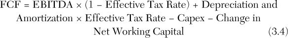
The definitions of FCF in Equations 3.3 and 3.4 are equivalent. As shown in Appendix 2B in Chapter 2, calculating the CFFO includes an adjustment for such noncash expenses as depreciation and amortization and income taxes paid.6 The only item excluded from EBITDA but included in CFFO is the after-tax interest expense, which is separately added back in Equation 3.3 to unleverage the CFFO. Net capital investments in Equation 3.3 and the sum of capex and the change in net working capital in Equation 3.4 capture the same thing: the required capital investments (to make the two equations identical, capex in Equation 3.4 should be estimated net of proceeds from sales of PP&E). Thus, provided that the analyst has access to all the necessary data and makes the same assumptions when using Equations 3.3 and 3.4, the FCF is the same no matter which definition is used.
Some analysts use EBIT rather than EBITDA as a starting point for the calculation of FCF. In this case, they often use the following definition of FCF:

The first component of Equation 3.5 is sometimes called net operating profit after taxes, or NOPAT. Again, as long as the same assumption is made regarding income taxes in Equations 3.4 and 3.5, the FCF is the same whether the analyst starts with EBITDA or EBIT.7
2.1.3. The Appropriate Discount Rate
One of the dilemmas involved in implementing a DCF model is selecting an appropriate discount rate. A widely accepted principle in corporate finance is that the cost of capital for an investment is the rate of return investors require. If the providers of capital do not receive a fair rate of return to compensate them for the risk they are taking, they will move their capital in search of better risk-adjusted returns. At a minimum, the cost of capital must equal the investors’ opportunity cost, or the rate they could earn on other risk-equivalent investments. This minimum rate of return is sometimes referred to as a hurdle rate, in that it represents the threshold return that must be earned to justify the investment from an investor’s perspective (to have a positive net present value, or NPV).
In the case of an acquisition, there are two schools of thought as to the appropriate discount rate to use when valuing a target: (1) the target’s hurdle rate and (2) the acquirer’s hurdle rate. Academicians recommend using a target’s hurdle rate to best match the riskiness of the company’s FCF with the riskiness implied by the discount rate. However, some practitioners frequently use a hurdle rate based on the acquirer’s hurdle rate or some desired rate of return.
2.1.3.1. The Target’s WACC
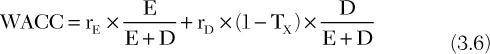
Under the FCF to the firm model, the appropriate hurdle rate is the target’s weighted average cost of capital (WACC). The WACC is defined as follows:8
where
rE = the target’s cost of equity, usually calculated using the capital asset pricing model (CAPM):
where
rF = the risk-free rate of return. In countries where the credit quality of the bonds issued by the sovereign (national) government is very high and the likelihood of sovereign default is extremely low, the risk-free rate of return is proxied by the yield to maturity on sovereign bonds. Because the investment horizon when valuing a target is usually long, analysts often consider sovereign bonds with long maturities, although this is not always the case. For example, in the United States, it is common to proxy the risk-free rate of return by the yield to maturity on 10-year (or longer maturities) Treasury bonds.9
β = a measure of the target’s systematic risk (or undiversifiable risk), which can be obtained from data vendors such as Barra, Bureau van Dijk (Orbis), Morningstar (Ibbotson), Thomson Reuters (Worldscope), or Value Line.10
ERP = the equity risk premium (also called market risk premium) required on a well-diversified portfolio of equity securities.11 Based on data for the 1900–2010 period, Dimson, Marsh, and Staunton (2011) estimated the equity risk premium in 19 countries. They reported an average equity risk premium of 3.8 percent, ranging from 2.0 percent in Denmark to 5.9 percent in Australia. It was 4.4 percent in the United States.12
E = the target’s market value of equity, measured by its market capitalization, or its stock price multiplied by the number of shares outstanding.
D = the target’s market value of debt. For publicly traded debt such as bonds, the market value is measured by multiplying the bond price by the number of bonds outstanding. For privately held debt such as bank loans, the market value is usually proxied by the book value, i.e., the latest value reported in the balance sheet.13
rD = the target’s cost of debt. If the target has issued bonds, the cost of debt is measured by the yield to maturity on the bonds. If no bonds are outstanding, the target’s cost of debt can be proxied by the yield to maturity on the bonds of comparable companies with the same credit quality (or credit rating). Alternatively, some analysts use the interest rate on the company’s debt, identifying the different layers of debt in the target’s capital structure whenever possible.14
Tx = the target’s tax rate, typically measured by the effective tax rate, i.e., the ratio of the income tax expense divided by the income before tax, obtained from the pro forma income statement.
In words, a target’s WACC is its cost of equity weighted by the proportion of equity in its capital structure, plus its cost of debt weighted by the proportion of debt in its capital structure; it represents the overall cost of the funds the target uses. The WACC must be calculated on an after-tax basis. Because interest is tax deductible, rD is multiplied by 1 minus the tax rate to reflect the interest tax shield.
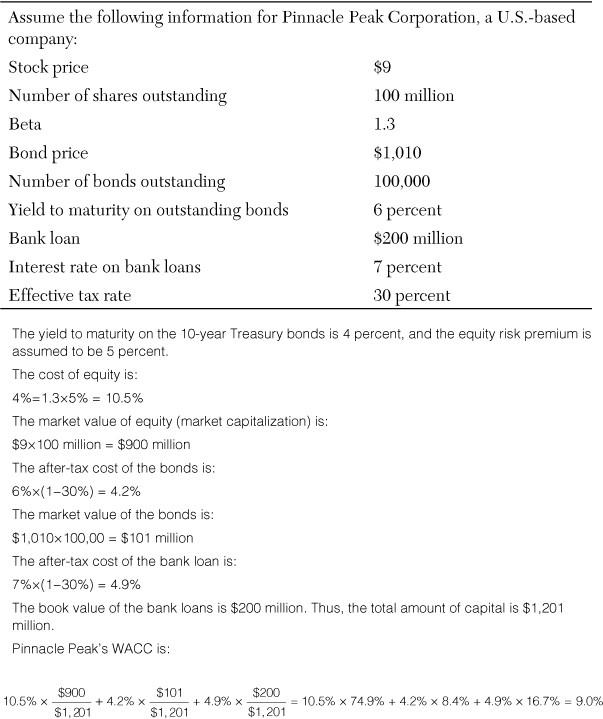
Exhibit 3.3 illustrates the calculation of the WACC of a hypothetical company.
Implicit in this discussion is the assumption that a target’s capital structure, and hence WACC, remains relatively constant over time.15 When material changes in capital structure occur, the WACC should be recalculated after each change. Debt is cheaper than equity because it has a more senior claim on assets and because interest is tax deductible, whereas dividends are not. As more debt is added to a company’s capital structure, the WACC declines with the increased use of financial leverage until the costs associated with the higher risk of default outweigh the benefits provided by the interest tax shield. Material changes in capital structure are likely to occur in transactions such as LBOs. Practically, recalculating the WACC after each change in capital structure results in a problem of circular logic: The future market value of equity is required to recalculate the WACC, but the WACC is needed to assess the future market value of equity. Consequently, when changes in capital structure are expected to be immaterial, analysts usually make the simplifying assumption of a constant WACC. An easier alternative than recalculating the WACC after each change in capital structure is to value the target using the adjusted present value method, which is discussed in Chapter 4.
2.1.3.2. The Acquirer’s Hurdle Rate
From the perspective of many acquirers, the appropriate discount rate to value a target is the acquirer’s WACC or some desired rate of return. Proponents of this approach argue that investment capital is a scarce resource and that the acquirer must choose only acquisitions that provide a rate of return that exceeds the acquirer’s WACC. Although not theoretically defensible, this viewpoint is widely held among practitioners and reflects the notion that most acquirers prefer to select projects with the highest NPV, not just those with positive NPVs.
When the target and the acquirer operate in the same or a related industry, their WACCs are likely to converge. Consequently, which discount rate is used might be relatively immaterial to a target’s value. However, when the target and the acquirer operate in different industries, with corresponding differences in the riskiness of their cash flows, these rates of return can diverge considerably, with a material effect on the target’s value. Exhibit 3.4 illustrates the risks the acquirer faces when using its own hurdle rate to discount the target’s FCFs.

If the acquirer uses its own hurdle rate and that hurdle rate is the same as the target’s WACC—say, 10 percent—the valuation of the target is unaffected at $496,619. If the acquirer’s hurdle rate is 2 percentage points higher than the target’s WACC, the acquirer will undervalue the target; it will estimate the target’s value to be $475,783 when its fair value is $496,619. Thus, it is likely to offer too little to the target’s shareholders, reducing the likelihood of being able to acquire the company and potentially missing out an opportunity to create value. A likely consequence of this practice is that the acquirer will tend to accept only acquisitions in which the target’s cash flows are riskier than its own cash flows—unless, of course, some form of market mispricing is present. In contrast, if the acquirer’s hurdle rate is 2 percentage points lower than the target’s WACC, the acquirer will overvalue the target. Thus, it will likely overpay for the target and provide yet another case of the winner’s curse.
2.1.4. The Continuing Value
One of the dilemmas facing the analyst when implementing a DCF model is the question, “For how many periods can I reliably forecast a target’s FCFs?” As noted earlier, whatever the length of the forecasting period, the decision ultimately involves a trade-off between the effect of the two components of the target’s operating value: the forecast of the periodic operating cash flows and the forecast of the continuing value.
The continuing value is an estimate of the target’s future FCFs for all periods beyond the forecasting period. It is a proxy for the aggregate future FCFs that the analyst feels unable or uncomfortable forecasting on a period-by-period basis. As with each of the individual forecasted periodic FCFs, the continuing value is discounted back to the present. As a practical matter, the longer the forecasting period, the smaller the weight of the continuing value in the target’s operating value, largely as a consequence of the discounting process. When the forecasting period is short, or when a target’s FCFs during the forecasting period are small or negative, which can happen for a start-up venture, the continuing value can constitute the majority (or even all) of a target’s operating value.
The two most widely used methods to calculate the continuing value are these:
• The exit multiple method
• The perpetuity growth method
2.1.4.1. The Exit Multiple Method
The continuing value can be viewed as the value that an acquirer can reasonably expect to receive if the target is sold at the end of the forecasting period. Under the exit multiple method, the analyst uses a multiple—for instance, the forward P/E ratio—to assess the implied price at which the target can realistically be sold, using an approach that is similar to the one described for earnings multiples. This implied price is then discounted back to the present using the appropriate discount rate.
The exit multiple method is commonly implemented with any of the following metrics:
• The price-to-earnings ratio
• The price-to-EBITDA ratio
• The price-to-sales ratio
No matter which metric is used, the continuing value is calculated by multiplying the final period estimate of the target’s permanent earnings by the forward multiple. Different industries and analysts use different exit multiples. The P/EBITDA ratio is a popular exit multiple among practitioners, but the P/sales multiple is more commonly used when the final period estimate of the target’s earnings or cash flow is expected to be negative or rather small.
To illustrate the exit multiple method, suppose that the pro forma financial statements of a target are prepared for five years and that the target’s fifth-year FCF is estimated to be $50,000. Furthermore, assume that the average forward P/FCF multiple for comparable companies in the target’s industry is 10. However, the analyst decides to adjust this multiple upward to 12 to reflect the higher growth rate in sales that is expected to arise as a consequence of integrating with the acquirer. Finally, assume that the target’s WACC is 10 percent. The forecasted continuing value is:
CV5 = 12 × $50,000 = $600,000
And the present value of the continuing value is:

2.1.4.2. The Perpetuity Growth Method
Under the perpetuity growth method, a target’s FCF is assumed to grow at some constant annual rate, g, in perpetuity. The analyst can extrapolate the growth rate of the target’s FCF from the historical and forecast growth rate of FCF. Such a growth rate might be high, however, and most analysts are unwilling to assume that a high growth rate is sustainable in the long run. Thus, they tend to use a lower growth rate, often in line with the expected long-term inflation rate plus sometimes 1 or 2 percentage points when they estimate that the target is well positioned to deliver some real growth in the long run.16
Under the perpetuity growth method, the continuing value is calculated as follows:17

where t is the number of periods in the forecasting period.
To illustrate the perpetuity growth method, we return to our earlier example, in which the pro forma financial statements of a target are prepared for five years, the target’s fifth-year FCF is estimated to be $50,000, and the target’s WACC is 10 percent. Furthermore, assume that the expected long-term inflation rate is 2 percent and that the target is a leader in its industry and can realistically deliver an additional percentage point of real growth per annum. The forecasted continuing value is:
And the present value of the continuing value is:

Both the exit multiple and perpetuity growth methods suffer from the same limitation: They assume that the riskiness and sustainability of a target’s earnings and cash flows are constant over time, which is not always realistic. This is why analysts tend to err on the conservative side when estimating continuing values. In addition, they usually perform sensitivity, scenario, and Monte Carlo simulation analyses to assess the effect of the continuing value on their valuation.
2.2. Estimating the Entity Value and Equity Value
After resolving the dilemmas regarding the length of the forecasting period and the calculation of the FCFs, discount rate, and continuing value, the analyst can estimate the target’s entity value and then its equity value.
2.2.1. The Entity Value
The entity value, also called firm value, represents the total value of the target. The largest component of the target’s entity value is usually its operating value, as defined in Equation 3.2. However, many analysts include two additional components when estimating a target’s entity value: (1) the amount of cash and marketable securities and (2) the market value of any nonoperating assets it owns. Thus, they define the target’s entity value as follows:

An acquirer that takes control of a company gains access not only to the target’s productive assets, but also to any cash and highly liquid short-term investments it has. In practice, the target’s cash and marketable securities are very often used to finance the acquisition.18
In addition, companies frequently make intercorporate investments—that is, they invest in other corporate entities for diversification or strategic purposes unrelated to their own operations. These intercorporate investments are usually not consolidated, but are accounted for using the equity method. The equity method does not itemize the affiliate’s revenues and expenses in the company’s income statement, but reports the affiliate’s earnings that accrue to the company as a nonoperating profit or loss. Thus, the cash flow effects associated with intercorporate investments are usually excluded from the calculation of a target’s CFFO. As a consequence, the value of these nonoperating assets is not reflected in either the present value of the target’s FCFs or its continuing value. To avoid understating a target’s entity value, analysts must add the market value of these (and any other) nonoperating assets to the target’s operating value.19 Among the other nonoperating assets that should be added to the target’s operating value are nonoperating assets carried on the balance sheet, the value of any unrecorded intangible assets unrelated to continuing operations, and the after-tax value of any overfunded pension plan assets carried off the balance sheet.
2.2.2. The Equity Value
The equity value reflects the value of the target from the common shareholders’ viewpoint. Thus, to derive a company’s equity value, it is necessary to subtract from the entity value the claims from all the stakeholders other than common shareholders. These claims typically include:
• The value of all debt, including interest-bearing debt (all types of short-term debt and long-term debt, including convertible debentures), capitalized leases, the capitalized value of operating leases, and the after-tax amount of any unfunded pension or post-retirement benefit liabilities20
• The value of any noncontrolling interest—that is, the company’s net worth (assets minus liabilities) that belongs to third parties, also called minority interest21
• The value of any equity-related securities that belong to stakeholders who have claims senior to the common shareholders’ claims (preferred stock, but also warrants and stock options)
• The value of any contingent claims, including the estimated value of any lawsuits and government actions
Thus, the target’s equity value is defined as follows:

The analyst can express the target’s equity value on a per-share basis by dividing it by the number of shares outstanding. The equity value per share represents an analyst’s best estimate of how much the target is worth from a shareholder’s viewpoint. In most instances, this per-share estimate represents the upper bound of value that an acquirer should be willing to pay for a target—paying a higher value would lower the acquirer’s expected rate of return below the discount rate and would destroy shareholder value.
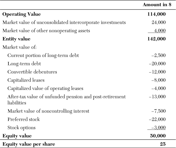
Exhibit 3.5 illustrates the calculation of the equity value for a hypothetical company.
To evaluate the reliability of the estimated equity value per share, the analyst can calculate an implied P/E ratio, as follows:

The implied P/E ratio serves as a validity check by comparing it to the adjusted industry average P/E ratio on a forward EPS basis for a set of comparable companies. If a target’s implied P/E ratio is above the adjusted average, it could indicate forecasting errors or biases in the pro forma analysis and suggest that the analyst revisit pro forma assumptions.
2.3. A Survey of Best Practices
A survey of leading practitioners (senior financial officers and financial advisers) conducted in the United States by Bruner, Eades, Harris, and Higgins in the late 1990s provides evidence of the “best practices” successful companies use for valuation purposes. The survey found the following:
• The dominant valuation method is the FCF to the firm model, but the vast majority of respondents regularly rely on earnings multiples as well, using both comparable companies and comparable transactions analyses. Practitioners weigh the different valuation methods depending on the purpose and type of analysis.
• The discount rate used in the FCF to the firm model is the target’s WACC. The relative weightings of a target’s debt and equity components are primarily assessed with the use of market (not book) values, using a company’s target (not current) capital structure.
• The dominant model for estimating a company’s cost of equity is the CAPM.
• When the cost of equity is being calculated using the CAPM, the risk-free rate is usually proxied by the yield to maturity on the 10-year (or longer maturity) U.S. Treasury bonds, largely because the yield curve is relatively flat beyond 10 years.
• Despite the fact that the CAPM calls for the use of a forward-looking beta (to reflect the uncertainty surrounding a target’s future cash flows), most respondents use a beta derived from historical data, obtained from data vendors such as Barra or from published sources.
• When estimating the equity risk premium, half of the financial advisers use an estimate of 7.0 to 7.4 percent, whereas nearly half of the senior financial officers use an estimate of 4.0 to 6.0 percent, causing the cost of capital estimates of financial advisers to frequently exceed those of the acquiring companies they advise.
• The vast majority of financial advisers use both the exit multiple method and the perpetuity growth method to estimate the continuing value.
• As discussed in Appendix 3 at the end of the chapter, when a multidivisional target is being valued, each division is valued separately using a distinct WACC. The values of all the divisions are then aggregated to arrive at the target’s entity value.
The survey conducted by Bancel and Mittoo in 2012 shows that “best practices” have not changed much in 14 years. When asked whether the global financial crisis that started in 2008 and the sovereign debt crises that followed affected the way they approach valuation, 55 percent of respondents said that those crises have not changed the way they value companies. However, the majority of valuation experts admit that the crises have affected how some of the variables are estimated. For example, 96 percent of respondents report making adjustments to the discount rate to incorporate the effects of liquidity, credit, and country/political risks. In addition, the survey shows that more than 80 percent of valuation experts perform Monte Carlo simulation analyses when valuing companies.
2.4. Cross-Border Considerations
When an acquisition involves companies from different countries, an additional set of considerations arises: country/political risk, expropriation risk, blocked funds risk, and foreign exchange (currency) risk, among others. These risks create additional uncertainty surrounding a target’s cash flows, so the analyst must consider them explicitly. As illustrated in the vignette at the beginning of this chapter, the materialization of any of these risks can significantly affect a company’s value.
Two approaches are typically used to incorporate the effect of these additional risks in the valuation: adjustments to the FCFs or adjustments to the discount rate. The first approach offers more flexibility because it adjusts the FCFs only if and when necessary. When investing abroad, particularly in emerging markets, companies frequently face expropriation and blocked funds risk. Expropriation risk refers to the risk that a foreign government will take over a target’s assets and operations, the risk that materialized for Repsol when the Argentinian government seized control of YPF. Blocked funds risk is related to repatriation constraints. Blocked funds, either partial or full, might still have considerable value to an acquirer, but only if the funds can be reinvested in the foreign country at favorable rates of return or if the acquirer’s objective is market share oriented. A classic example was the decision by McDonald’s to invest $40 million in the former Soviet Union in the early 1990s at a time when Russian laws prevented the repatriation of any profits. Obviously, McDonald’s Russian investment was motivated by the long-term view of growing its Russian operations, and repatriation of profits to the United States was not a short-term requirement.
When an acquirer and a target operate in different currencies, the analyst usually produces two sets of forecasts: one set for the acquirer and one set for the target. The target’s forecast FCFs are prepared using the target’s functional currency, with explicit consideration given to expropriation and blocked funds risks. The acquirer’s forecast FCFs are then prepared after the target’s forecast FCFs are translated into the acquirer’s functional currency. The conversion between the target’s currency and the acquirer’s currency requires an assumption with respect to the movement of exchange rates and, therefore, an explicit consideration of foreign exchange risk.
An alternative to incorporating the various risks in the valuation is to adjust the discount rate. In theory, the discount rate should be the risk-adjusted cost of capital of the target. As noted earlier, however, many acquirers use their own WACC or some desired (or required) rate of return (hurdle rate) for the purposes of discounting the target’s cash flows. To incorporate the effect of the uncertainties associated with cross-border acquisitions, many analysts believe that the appropriate way to account for these additional risks is to add a risk premium to the discount rate. For instance, some acquirers add a risk premium as high as 10 percentage points above their domestic hurdle rate. One objection to this approach is that it assumes that the degree of risk is uniform over the life of the target. Furthermore, because of the exponential nature of discounting, a uniformly higher discount rate (because of an add-on risk premium) substantially penalizes early cash flows and might not adequately reflect the risk in later periods.
Both approaches are used in practice, but many analysts prefer the first approach because it allows them to be more precise when modeling the effect of any additional risk. By preparing the target’s forecasts first, initially in the target’s functional currency and then in the acquirer’s functional currency, the analyst can explicitly incorporate expropriation and blocked funds risks, as well as country/political risk. Furthermore, the analyst can explicitly consider foreign exchange risk when translating the target’s FCFs into the acquirer’s functional currency.
Although cross-border transactions are typically more risky than domestic ones, companies should not shy away from them. These transactions often offer opportunities that are not available locally. In their analysis of approximately 26,000 M&As that took place between 1988 and 2010, Kengelbach and Roos (2011) found that, on average, acquirers experience higher returns on their cross-border transactions than on their domestic ones, particularly if the target is a public company located in an emerging market.
2.5. Illustration
We now return to Mattel to illustrate the use of the FCF to the firm model. We assume that we are at year end 2011 and that we want to estimate Mattel’s equity value per share. In Chapter 2, we analyzed Mattel’s financial statements between 2008 and 2011, and we made forecasts for 2012. We use these forecasts as a starting point for the valuation.
Before valuing Mattel, let us review the different steps of the FCF to the firm model:
1. Forecast the FCFs.
2. Estimate the appropriate discount rate that reflects the riskiness of the FCFs.
3. Estimate the continuing value.
4. Estimate the operating value by discounting the FCFs (from step 1) and the continuing value (from step 3) at the appropriate discount rate (from step 2).
5. Estimate the entity value by adding to the operating value (from step 4) the company’s cash and marketable securities and, if relevant, the market value of nonoperating assets.
6. Estimate the equity value by subtracting from the entity value (from step 5) the market values of debt, noncontrolling interest, equity-related securities other than common stock, and contingent claims.
7. Estimate the equity value per share by dividing the equity value (from step 6) by the number of shares outstanding.
As mentioned earlier, analysts typically forecast a company’s FCF for three to five years and capture the value of the following FCFs in the continuing value. To keep this valuation simple, we forecast the FCF for one year only (2012).
Step 1
In Chapter 2, we forecast Mattel’s pro forma income statement for 2012, but not its cash flow statement. Thus, we use a definition of FCF that starts with an earnings metric. We use operating income as a proxy for EBIT and apply Equation 3.5:22
FCF2012 = EBIT2012 × (1 − Effective Tax Rate2012) + Depreciation and Amortization2012 − Capex2012 − Change in Net Working Capital2012
The amounts for EBIT, the effective (income) tax rate, and depreciation and amortization for 2012 are taken from Mattel’s pro forma income statement in Exhibit 2.13. They are $1,072.3 million, 20.8 percent ($203.5 million divided by $976.9 million), and $166.1 million, respectively. Management indicated that it was expecting to spend between $215 and $225 million in capital expenditure in 2012; we use the higher estimate. The amounts to calculate the change in net working capital are taken from Exhibit 2.12. We assumed that the working capital ratios would remain constant between 2011 and 2012, inventories would increase from $487.0 million to $492.4 million, accounts receivable would decrease from $1,246.7 million to $1,217.9 million, and accounts payable would increase from $335.0 million to $428.5 million. The increase in inventories is a use of cash of $5.4 million, whereas the decrease in accounts receivable and the increase in accounts payable are sources of cash of $28.8 million and $93.5 million, respectively. Thus, the change in net working capital is a net source of cash of $116.9 million:
FCF2012 = 1,072.3 × (1 − 20.8%) + 166.1 − 225.0 + 116.9 = $907.1 million
Step 2
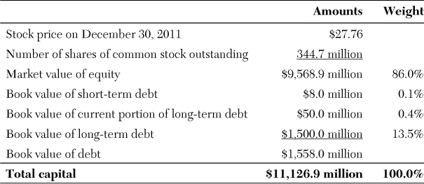
To estimate Mattel’s WACC, we first need to calculate the total amount of capital, i.e., Mattel’s market values of equity and debt. Mattel has bonds outstanding, but because the company’s use of debt is limited and the difference between the market and book values of debt is small, we use the book values reported on Mattel’s balance sheet at year end 2011 to proxy for their market values. Exhibit 3.6 provides the necessary data to calculate the total amount of capital.
Next, we need to estimate Mattel’s cost of funds. For the cost of equity, we rely on the CAPM and we use the beta provided by Value Line (0.9). As discussed earlier, we could proxy the risk-free rate of return by the yield to maturity on 10-year U.S. Treasury bonds at year end 2011 (1.9 percent), and we could use the historical equity risk premium estimated by Dimson et al. (2011) for the United States (4.4 percent). This would yield a cost of equity of 5.9 percent. It is clear, however, that 5.9 percent would underestimate the long-run required rate of return from investing in Mattel’s common stock. Although the company’s systematic risk (0.9) is lower than the market average (1.0), the cost of capital of a company such as Mattel should be closer to 10 percent than to 5 percent. Mattel’s cost of equity is low because the yield to maturity on U.S. Treasury bonds is unrealistically low. One of the consequences of the global financial crisis of 2008 was a “flight to safety”—many investors sold equities and bought sovereign bonds instead, pushing sovereign bond prices up and bond yields down. In addition, many central banks bought government bonds, in an effort to keep interest rates low and jump-start their faltering economies, thus maintaining the yields to maturity on government bonds at an historically low level. Although these conditions led to a lower cost of borrowing for companies such as Mattel, this situation is not likely sustainable in the long run; sooner or later, government bond yields will increase, leading to higher costs of borrowing. Thus, many analysts using the CAPM have been making upward adjustments, a practice that Bancel and Mittoo (2012) have identified. They have been doing so by using a higher value for the risk-free rate of return, a higher value for the equity risk premium, or a combination of both. However, because there is no theoretical model to justify such adjustments, there is little consensus on which method is best.
To reflect a more realistic long-run cost of equity for Mattel, we use a higher value for the risk-free rate of return. During the five years preceding the global financial crisis of 2008, the yield to maturity on 10-year U.S. Treasury bonds varied little, oscillating between 4.1 and 4.7 percent. We arbitrarily use 4.7 percent as a realistic, long-term proxy for the risk-free rate of return. Although the equity risk premium used in the CAPM should be forward looking rather than historical, there is no consensus on what the forward-looking equity risk premium might be.23 Thus, we use the 4.4 percent historical equity risk premium identified by Dimson et al. (2011) for the United States.
For the cost of debt, we use the estimates from Chapter 2: 0.4 percent for short-term debt and 6.9 percent for long-term debt.24 Exhibit 3.7 summarizes the data used to estimate Mattel’s cost of funds.

Using the information in Exhibits 3.6 and 3.7, we estimate Mattel’s WACC using Equation 3.6 as follows:
WACC = 8.7% × 86.0% + 0.4% × (1 – 20.8%) × 0.1% + 6.9% × (1 – 20.8%) × (0.4% + 13.5%) = 8.2%
Step 3
To estimate the continuing value that captures the value of Mattel’s FCFs from 2013 onward, we use the perpetuity growth model and apply Equation 3.8:

For the FCF in 2012 and the WACC, we use our estimates from steps 1 and 2, respectively. In addition, we assume a growth rate to perpetuity of 3 percent per annum. Thus:25
Step 4
We apply Equation 3.2 to estimate Mattel’s operating value:
Note that because we forecast the FCF for only one year, the continuing value represents 95.2 percent of Mattel’s operating value.
To estimate Mattel’s entity value, we apply Equation 3.9. At year end 2011, Mattel had $1,369.1 million of cash on its balance sheet. The company does not identify any nonoperating assets, such as equity stakes in unconsolidated subsidiaries, in its annual report. Thus, its entity value is simply the sum of its operating value and cash ($18,784.0 million).
Steps 6 and 7
We apply Equation 3.10 to estimate Mattel’s equity value. For interest-bearing debt, we use the book values reported in the company’s balance sheet at year end 2011 and identified in Exhibit 3.6. A review of the annual report indicates the following:
• There is no non-controlling interest.
• In addition to interest payments and debt repayments, Mattel faces contractual obligations, including $2.4 million of capitalized leases, $472.8 million of capitalized value of operating leases, $379.3 million of defined benefits and post-retirement liabilities, and $719.7 million of other types of firm commitments.
• No preferred stock is outstanding.26 However, Mattel has an equity and long-term compensation plan, and restricted stock units and stock options are outstanding. The fair value of these equity-related securities is estimated at $361.8 million.
• There are no material contingent claims.
Exhibit 3.8 shows the estimation of Mattel’s equity value per share based on the number of diluted shares outstanding at year end 2011.27
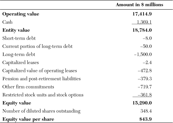
Based on our assumptions, Mattel’s fundamental value is approximately $44 per share. Of course, our valuation is sensitive to quite a few assumptions made when estimating the FCFs, WACC, and continuing value. One of the most critical assumptions is the growth rate to perpetuity. This growth rate is a key driver of the continuing value, which is itself the largest component of Mattel’s entity value. To assess how sensitive our valuation is to this assumption, we can perform a sensitivity analysis and estimate what Mattel’s equity value per share would be for growth rates to perpetuity ranging from 0 percent to, say, 5 percent. Exhibit 3.9 reports the results of such a sensitivity analysis.
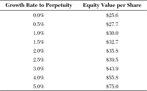
Exhibit 3.9 confirms that Mattel’s value is extremely sensitive to the growth rate to perpetuity. For example, if FCFs were growing at 2 percent rather than 3 percent per annum, the equity value per share would be 18.3 percent lower.
At year end 2011, Mattel’s stock price was $27.76. Assuming that our model is a reliable way of estimating Mattel’s fundamental value, we can determine the implied growth rate to perpetuity—that is, the growth rate that would make Mattel’s equity value per share equal to its stock price. According to Exhibit 3.9, this implied growth rate is approximately 0.5 percent. Put another way, Mattel looks fairly valued if it can deliver a modest growth of 0.5 percent per annum. An analyst might be tempted to conclude that, in light of Mattel’s growth potential, the company seems undervalued. Because our model is very basic, this conclusion would be premature at this stage; any analyst whose task is to value Mattel would build a more refined model than the one we presented here before reaching any conclusion. In addition, the analyst would likely perform a Monte Carlo simulation analysis to fully explore how the key inputs jointly affect Mattel’s value.
Summary
In this chapter, we reviewed the two most frequently used methods of valuing a company: earnings multiples and the FCF to the firm model. Although earnings multiples are acceptable to value small share-block purchases, a more thorough analysis—as provided by a DCF model—is preferable when substantial amounts of capital are involved.
Implementing the FCF to the firm model requires the analyst to resolve a number of operational dilemmas related to the length of the forecasting period and the estimation of the FCFs, WACC, and continuing value. It is also important that these estimations incorporate the risks that can potentially affect the target’s value. After resolving these dilemmas, the analyst can start building the valuation model. Because the valuation is sensitive to the assumptions made along the way, it is critical that the analyst use current, relevant data to define assumptions. In addition, the analyst must keep records of the choices made and the basis for these choices. After building the model, the analyst should perform sensitivity, scenario, and Monte Carlo simulation analyses to clearly identify the key assumptions that drive the target’s value. One always needs to remember that a model’s output (the target’s value) is only as good as its inputs (assumptions)—what practitioners refer to as model risk.
Endnotes
1. Schreiner (2007) reports that forward earnings multiples provide more accurate valuations than trailing earnings multiples. Moreover, Liu, Nissim, and Thomas (2002, 2007) show that forward P/E multiples outperform not only trailing P/E multiples, but also cash flow multiples and sales multiples.
2. Namco’s profitability deteriorated between 2008 and 2010; the company made a profit of more than ¥30 billion in 2008, but a loss of approximately ¥30 billion in 2010. In 2009, Namco initiated a restructuring plan that is proving successful. However, it took three years for profit to recover; net income in 2011 was positive but small, which explains why the trailing P/E ratio is abnormally high.
3. On 30 December 2011, Mattel’s share price was $28. Thus, based on the average forward P/E ratio, the company appears fairly valued.
4. The effect of the interest tax shield is already reflected in the pro forma CFFO because income taxes are calculated on a cash basis (adjustments are made for the change in deferred income taxes and income taxes payable).
5. Equation 3.3 assumes that interest paid is reported in CFFO. This is always the case under U.S. Generally Accepted Accounting Principles (GAAP), but not necessarily under International Financial Reporting Standards (IFRS). IFRS gives preparers the choice of reporting interest paid as part of their operating or financing activities. If interest paid is not included in CFFO, the first adjustment is not necessary. If the company reports under IFRS, the analyst should also check where dividend and interest received are included. If they are in CFFO, as required under U.S. GAAP, no adjustment is necessary. If dividend and interest received are reported as part of the company’s investing activities, they should be added back to CFFO before calculating the FCF. A study by Gordon, Henry, Jorgensen, and Linthicum (2012) shows that 77 percent of companies reporting under IFRS include interest paid in CFFO, but only about half of these companies include dividend and interest received in CFFO.
6. The second component in Equation 3.4 is the depreciation and amortization tax shield. Because the depreciation and amortization expense is subtracted before income taxes, it reduces the amount of taxable income and, thus, the income tax expense. This tax benefit must be included in the calculation of the FCF.
7. Because companies often use different depreciation methods for financial reporting and tax purposes, the difference in depreciation methods leads to a difference in income taxes, which is reflected in the balance sheet as deferred income taxes. Some analysts take into account the effect of this difference on the company’s FCF by adding the change in deferred income taxes in Equations 3.4 and 3.5.
8. Equation 3.6 assumes that the target has only common equity outstanding. If it also has preferred equity outstanding, the WACC must be reformulated as follows:
where
rP = the cost of preferred equity, usually calculated as the dividend per share divided by the preferred stock price.
P = the market value of the target’s preferred equity, measured as the preferred stock price multiplied by the number of preferred shares outstanding.
9. In countries where the likelihood of sovereign default is not negligible, or where the sovereign government does not issue bonds in domestic currency with long maturities, finding a proxy for the risk-free rate of return is problematic. A suitable alternative is to use the yield to maturity on corporate bonds of the highest credit quality (Aaa by Moody’s, or AAA by Standard & Poor’s and Fitch) issued in domestic currency with long maturities.
10. Some analysts prefer to construct their own measure of the target’s systematic risk. Appendix 3 describes alternative methods they can use to do so.
11. Although we prefer to define the CAPM as the risk-free rate of return plus the company’s beta times the equity risk premium, an alternative definition of the CAPM is:
rE = rF + β × (rM – rF)
where rM is the market’s return, which is typically proxied by the return on a market index, such as the S&P 500 in the United States.
12. Dimson et al. (2011) use different approaches to calculate the equity risk premium. For the risk-free rate of return, they use the yield to maturity on long-maturity as well as on short-maturity government bonds. They calculate the average using both an arithmetic as well as geometric mean. The results reported here are those using the yield to maturity on long-maturity government bonds and a geometric mean.
13. The proxy for D ignores many common forms of debt, such as operating leases, pensions, and other post-retirement benefits. When these alternative forms of debt are immaterial in amount, they can be ignored.
14. Most companies provide a breakdown of their borrowings in the footnotes to the financial statements. For each significant layer of debt, they often identify the amount, the interest rate, and the maturity. They might also provide an estimate of the weighted average cost of debt.
15. Some analysts prefer to estimate the WACC for a target capital structure rather than the current capital structure. This approach has the advantage of anticipating future material changes in capital structure that could affect the target’s value. For example, if an acquirer is planning to change a target’s level of debt after the acquisition, the target’s value should be calculated twice: once using the current WACC assuming no debt change and once using the revised WACC reflecting the debt increase. The difference between the two values represents the potential increase in the target’s value due to the increase in financial leverage. If the additional debt can be raised only as a consequence of the acquisition, the increase in value represents a potential synergy.
16. The unwillingness of most analysts to assume a high growth rate in the long run essentially reflects the concern that, over time, above-average rates of return revert back to a mean value (the phenomenon of mean reversion).
17. The relevant FCF for the continuing value is the next year’s FCF, not the current year’s FCF. Indeed, the continuing value reflects all the FCFs that the company will generate in the future. The current year’s FCF has already been integrated in the company’s operating value. Thus, the first FCF to include in the continuing value is the next year’s FCF, not the current year’s FCF.
18. Conventional wisdom suggests that companies with large amounts of cash on their balance sheet are likely targets because they are attractive to other companies that are interested in gaining access to this cash. However, research by Harford (1999) and Pinkowitz (2002) shows the opposite. These authors conclude that cash-rich companies are better equipped to defend themselves against unsolicited acquisitions.
19. When the values of intercorporate investments and other nonoperating assets are immaterial in amount, analysts frequently use the reported book values as a proxy for their market values.
20. Relying on the market values of debt instruments is better than relying on their book values. However, when the amount of debt relative to equity is small or the debt is privately held, using book values is acceptable. Capital (finance) leases are included in the balance sheet, but operating leases are not. Information about a company’s pension and post-retirement benefits is usually provided in the footnotes of the financial statements, although the quality of disclosure varies among countries and companies.
21. When the value of noncontrolling interest is immaterial, the book value is an acceptable proxy for the market value.
22. Taxes such as payroll taxes are including in operating income but not in EBIT. However, the difference between operating income and EBIT is usually small.
23. In late 2001, following the burst of the dotcom bubble, the Research Foundation of CFA Institute gathered a group of experts to discuss the equity risk premium. At the time, estimates for the equity risk premium ranged from 0 to 7 percent, with an average of 3.7 percent. Ten years later, the Research Foundation revisited the topic of the equity risk premium and asked some academicians and practitioners to provide estimates of the forward-looking equity risk premium. Although some variations arose, most of these experts provided an estimate of around 4 percent. For more information about the different approaches used to forecast the forward-looking equity risk premium, see Research Foundation of CFA Institute, 2011.
24. Using a cost of equity of 5.9 percent and a pre-tax cost of long-term debt of 6.9 percent would also lead to an inconsistency. Because investing in a company’s common stock is more risky than investing in its debt, the cost of equity should logically be higher than the pre-tax cost of debt. As mentioned previously, this inconsistency arises because the yields on government bonds are unrealistically low.
25. All the calculations were performed in Excel, without rounding any of the intermediate results. Thus, slight differences might arise between the numbers reported and the ones obtained with a calculator.
26. Mattel is authorized to issue shares of preferred stock, but none is outstanding at year end 2011.
27. The number of diluted shares outstanding includes the 3.7 million shares that would be added if the stock options were exercised. If Mattel were the target of an acquisition, the acquirer would likely extend its offer to the restricted stock units and the stock options.
Appendix 3: Some Frequently Asked Questions and Answers About the Free Cash Flow to the Firm Model and Earnings Multiples
Valuation is an art to be learned. In many respects, it lacks the precision associated with valuing a plain vanilla (fixed-coupon, option-free) bond or other fixed-return financial asset in which the future cash flows are relatively certain. Few absolute principles apply when valuing a target; however, rules of thumb abound. Consequently, we address in this appendix some of the frequently asked questions about DCF models and earnings multiples.
1. How can I use the free cash flow to the firm model to value a multidivisional company?
Ideally, the best way to implement the FCF to the firm model in a multidivisional company is to model the future performance of each division separately, apply a distinct WACC representative of the riskiness of each division, and then sum the individual values to arrive at an aggregate entity value. This approach is sometimes referred to as the break-up method or the sum-of-the-parts method. This analysis is particularly instructive for conglomerates and holding companies as they try to assess whether greater shareholder value is created when the individual business units are operated as a single entity or on a stand-alone basis. Recall from Chapter 1 that conglomerates and holding companies usually trade at a 13 to 15 percent discount relative to focused companies.
2. Which discount rate should I use to value a foreign acquisition?
The “best practices” answer is always the same: Use the discount rate that best reflects the riskiness of the company’s free cash flows. However, the survey results of Graham and Harvey (2001) are enlightening. When asked how frequently companies use the following discount rates when evaluating a new project in an overseas market, the respondents indicated “always or almost always” as follows:
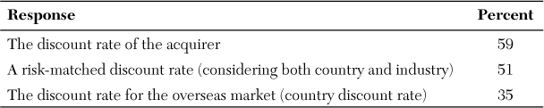
Thus, although some acquirers do try to match the discount rate to the particular country/industry risk profile, many do not. The obvious question then is whether these companies fail to undertake appropriate acquisitions because of using an inappropriate discount rate.
3. I have heard about leveraged and unleveraged betas. What is the difference between them, and which one should I use in the capital asset pricing model (CAPM)?
A company is subject to two types of risk: business risk, which is the risk associated with its operations, and financial risk, which is the risk associated with its capital structure (specifically, the amount of debt relative to equity). As a consequence, it is possible to identify two different betas:
• The leveraged beta, also called equity beta, reflects the systematic component of a company’s business risk and financial risk.
• The unleveraged beta, also called asset beta, reflects the systematic component of its business risk only.
If a company does not have any debt in its capital structure, the leveraged and unleveraged betas are identical. If the company is financed with a mix of debt and equity, however, the leveraged beta will be higher than the unleveraged beta. Indeed, the higher the financial leverage, the higher the financial risk and, therefore, the higher the leveraged beta.
The connection between the levered beta (βL) and unleveraged beta (βU) is given by the following equation:
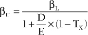
where D and E represent the market values of debt and equity, respectively, and D/E reflects the debt-to-equity ratio. TX is the tax rate.
Although understanding the distinction between the leveraged beta and the unleveraged beta is important, the effect of choosing one over the other on the company’s value is usually minimal unless the company is highly leveraged.
4. How can I estimate my own beta?
Some analysts prefer to construct their own measure of the target’s systematic risk. A first method is to perform a regression analysis using historical data. The dependent variable is the target’s excess return, i.e., the difference between the target’s stock return and the risk-free rate of return. The independent variable is the market’s excess return, i.e., the difference between the market’s return and the risk-free rate of return. The target’s beta is given by the slope of the regression. This method requires access to past market data. It is sensitive to the periodicity of the market data (monthly, weekly, daily), the length of the estimation window, and econometric choices.
A second method is to perform a comparable company analysis, much like the approach taken for earnings multiples, and to apply the following steps:
1. Identify a group of comparable companies.
2. Obtain the following data for each of the comparable companies: βL, D, and E. Data vendors provide leveraged betas that reflect both the company’s business and financial risk.
3. For each comparable company, calculate the unleveraged beta, which reflects only the company’s business risk. To move from the leveraged to the unleveraged beta, the effect of financial leverage (considering the interest tax shield) must be excluded as follows:

4. Calculate the average unleveraged beta for the group of comparable companies (βU*).
5. Assuming that the target’s unleveraged beta is equal to the industry’s average unleveraged beta, estimate its leveraged beta. To do so, the effect of the target’s financial leverage (considering the interest tax shield) must be included as follows:
A third method is simply to use the industry beta, which is typically more stable and reliable than company betas. A rule of thumb some analysts follow is to use the industry beta if the target’s beta from several sources varies by more than 0.2, indicating a high degree of instability and potential unreliability in the target’s beta.
5. How can I estimate the capitalized value of operating leases, and how does it affect the calculation of a company’s WACC?
Most debt instruments are reported in the balance sheet, and so are capital (or finance) leases. In contrast, operating leases are carried off balance sheet. Thus, the analyst must be able to capitalize the present value of the future operating lease payments to the balance sheet. Operating lease payments are usually disclosed in the footnotes to the financial statements, so estimating the capitalized value of operating leases is relatively straightforward: It requires discounting the future operating lease payments. Most analysts use the company’s long-term cost of debt (or the average rate implicit in the leases, if known).
Let us return to the example of Pinnacle Peak Corporation presented in Exhibit 3.3. Assume that a review of the footnotes reveals that the company has operating leases carried off balance sheet and that the implicit cost of lease financing is 8 percent. The future operating lease payments are as follows:

The present value of the future operating lease payments and, thus, their estimated market value can be calculated as follows:

If the capitalized value of operating lease payments is added to Pinnacle Peak’s amount of debt and equity estimated in Exhibit 3.3, the total amount of capital increases from $1,201.0 million to $1,425.8 million. The after-tax cost of lease financing is 5.6 percent, so Pinnacle Peak’s WACC becomes:
10.5% × 63.1% + 4.2% × 7.1% + 4.9% × 14.0% + 5.6% × 15.8% = 8.5%
Note that including the capitalized value of operating lease payments increases Pinnacle Peak’s proportion of debt relative to equity by 11.8 percentage points (from 25.1 percent to 36.9 percent) but lowers the company’s WACC by 50 basis points (from 9.0 percent to 8.5 percent). This is because debt is cheaper than equity; as the proportion of debt increases, the WACC decreases. This holds true as long as the cost of financing on the bonds and the bank loans remains unchanged because the increase in financial leverage brings only benefits: cheaper funds. In reality, financial markets and institutions tend to require a higher yield as financial leverage increases to compensate them for the additional credit risk. At some point, the incremental cost of financing outweighs the incremental benefit provided by the additional debt. This is why it is important for the financial community in general and analysts in particular to capitalize the value of operating lease payments, to get a full understanding of a company’s true amount of financial leverage and appropriate cost of funds—unless, of course, the amount of operating leases is not material.
6. Using the price-to-earnings (P/E) ratio to value a company is straightforward. However, some companies have a higher multiple than others. Why is it often said that a high P/E ratio indicates high future growth?
Two components drive the future value of a company (and, thus, its stock price): the company’s value excluding any growth opportunities, and the value of the future growth opportunities. Suppose that a company has invested in several projects that will generate positive free cash flows in the future. According to the dividend discount model (DDM), a widely used model for valuing equity securities, the present value of a company, as captured by its stock price, is equal to the present value of its future dividend payments discounted at the cost of equity:

Here, P0 is the current stock price, Dt is the dividend per share, and rE is the company’s cost of equity.
To simplify Equation (I), let us assume that, in the future, the dividends payments will be constant. Thus, Equation (I) represents the present value of a perpetuity and collapses to the following:

According to this equation, a company can maximize shareholder value by distributing 100 percent of its earnings as dividends. If the company does so, the dividend per share is equal to the earnings per share (EPS), and Equation (II) becomes:

Now suppose that the company has another investment opportunity that will generate a positive net present value. As a consequence of the new project, Equation (III) becomes:

Here, NPVGO is the net present value of the investment (growth) opportunity. Equation (IV) shows that two components are now driving the value of the company: the value of the company excluding any new growth opportunity (first term of the equation), and the value of the new growth opportunity (second term).
If we divide Equation (IV) by EPS, it becomes:
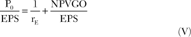
The left side of this equation is simply the P/E ratio. The right side shows that a company’s P/E ratio is related to two elements: the company’s cost of equity and the net present value of its future growth opportunities. The higher the company’s cost of equity (that is, the higher the risk of the stock), the lower the company’s P/E ratio. In contrast, the higher the company’s NPVGO, the higher the P/E ratio.
Equation (V) helps us understand why some companies with low earnings have a high P/E ratio, whereas other companies with high earnings carry a low P/E ratio. The difference in P/E ratios is driven not only by the level of earnings, but also by the level of the future growth opportunities.
Note that, because it refers to the future, NPVGO measures the market’s expectation with regard to a company’s growth opportunities. Therefore, it is more correct to say that a high P/E ratio indicates a high expectation of growth.