
3. Financial Forecasting
3.1 Introduction
As we stated in Chapter 1, “Introduction,” the objective of this book is to develop a set of valuation frameworks that will enable a business manager to quantify the value implications of business decisions. Those business decisions can range from building a new manufacturing facility to developing a new product to acquiring a firm.
The foundation of all valuation frameworks in finance is the present value relation:
Here, E(CF1), E(CF2), and so on are expected future cash flows, r denotes a discount rate, and Value0 is the value of the project that we are trying to measure. There are two key pieces of information needed to evaluate this present value relation and measure the value implication of a business decision. The first is the expected future cash flows that would result from the decision. The second is the discount rate, which reflects the riskiness of the future cash flows (and, therefore, the risk entailed in the decision), which is used to discount the expected future cash flows and transform them into a value amount today.
We will begin by developing a method to determine expected future cash flows. As mentioned in Chapter 1, any project can be put in the context of a balance sheet. In fact, the project can be thought of as a series of balance sheets, with each one representing the state of the project at a different point in time. As you learned in Chapter 2, “Financial Statement Analysis,” the change from one balance sheet to the next can be captured in an income statement, a cash flow statement, and/or a sources and uses of cash statement. Therefore, the project can be thought of as a series of balance sheets, income statements, and different types of cash flow statements. To evaluate Equation 1, we need to develop expected future cash flows. The obvious place to calculate them is from the series of balance sheets, income statements, and especially the cash flow statements that represent the business decision. In this chapter, we explain how to develop these future, or projected, financial statements. We specifically focus in this chapter on how to develop these projected financial statements for a business, but keep in mind that the techniques described here will work for any type of business decision.
So, in this chapter, you will learn how to project a firm’s financial statements into the future. We explain projections for growth of the entire firm and how to plan the launch of a new project. We will continue using the example of ABC Company to illustrate precisely how financial forecasts are put together.
3.2 Constructing Pro Forma Financials
Firms need to plan for the future. Plans need to be made both for the overall growth path of the firm and for new initiatives that may be launched. Looking into the future is necessarily difficult because it inherently involves a great deal of uncertainty. However, recognizing this uncertainty and making logical and well-reasoned assumptions about likely outcomes allows the firm to deal intelligently with the need to plan for the future.
A firm constructs pro forma financials to project financial conditions into the future. In the most basic sense, pro forma financials are the balance sheet and income statements extended out for a certain period of time, often five years. Making these projections allows a firm both to see the implications of future growth and to think carefully about how to finance expansion. For example, if a firm wants to grow, it will need to obtain funds for things such as buying inventory, hiring additional employees, and buying or leasing new space if needed. It can get the needed capital by borrowing, issuing equity, or retaining earnings. The pro forma financials give the firm both an idea of the size of the funding needed for future growth and the ways in which those funds could be obtained.
Constructing these statements is fairly straightforward. First, we make assumptions about how certain key components of the financial statement will grow in the future. Second, we extrapolate out the other components of the balance sheet based on our basic assumptions. Finally, we add in a financing path showing where any needed funds will come from. After these basic pieces have been set down, we use some of the financial ratios discussed in the previous chapter to evaluate whether the projected growth path is sustainable. If it is not sustainable, we need to revisit some of the assumptions made in the first step and repeat the projection exercise. If it is sustainable, the firm can use the pro forma financials as a guide for activities and decisions in the near term.
3.2.1 Creating the Pro Forma Worksheet
In this chapter, we’ll create pro forma financials for ABC Company, continuing the example that we started in Chapter 2. Figure 3.1 provides the format that we will use. We’ve split the figure into three parts to make it easier to read. (Figure 3.1a provides explanations of how to calculate the various components of the pro forma financial statement.) We’ve also combined some of the accounts that appeared in the income statement in Figure 2.4 to streamline the accounts and focus on the most important aspects of putting together our forecast. Indeed, in reality, financial statements are very complex, and each presents aspects unique to each individual firm. Here, we take a high-level view, thus providing an approach applicable to the vast majority of firms.


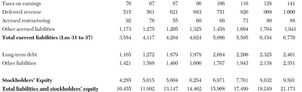

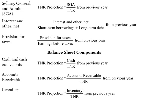
The numbers in the first three columns of Figure 3.1.1 are identical to those in the balance sheet and income statement tables in Chapter 2, but they are reorganized in a way that will be useful for constructing the pro forma financial statements. Both the income statement and balance sheet are combined here so that the link between the two financial statements is very clear as we create financial projections.
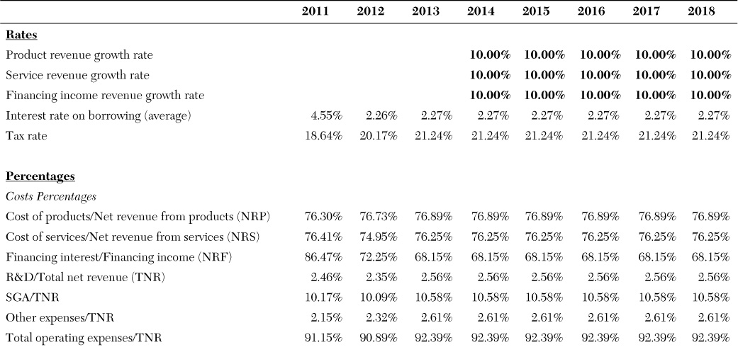
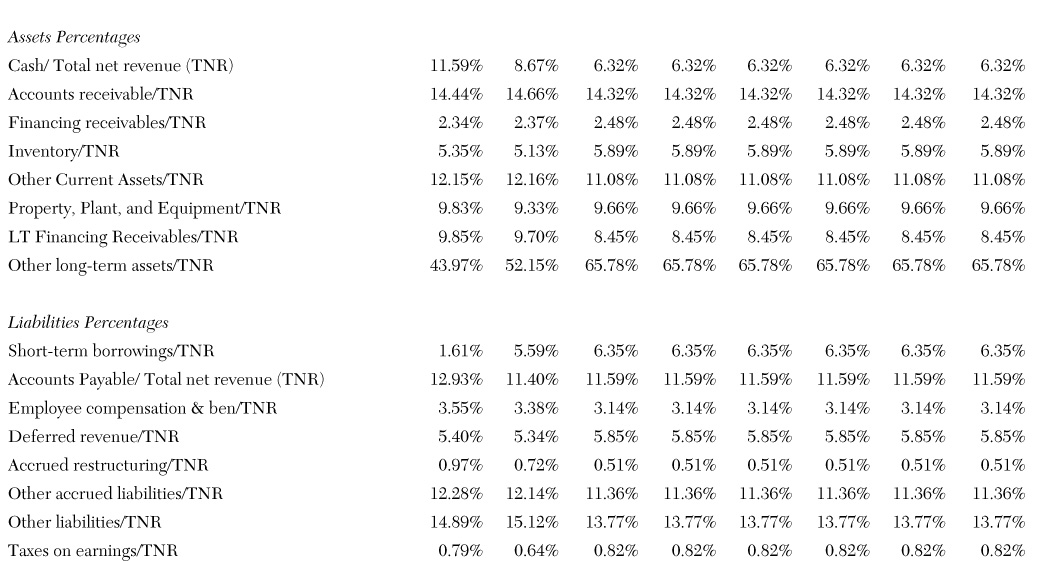
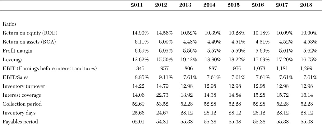
In Figures 3.1.2 and 3.1.3 are three new sections. The top section of Figure 3.1.2 contains a set of rates that are our assumptions about the future growth of ABC. The bottom half shows a set of percentages that will be used for constructing the individual pieces of the financial forecast. Figure 3.1.3 contains many of the financial ratios from Chapter 2; these will be used to evaluate the strengths and weaknesses of our planned path for growth.
3.2.2 Rates
The section in Figure 3.1.2 titled Rates contains the key assumptions for making a financial forecast. The top three lines show some important assumptions about the future growth path of ABC. They set out the assumptions we’ll make about the rate of growth of revenue from products, services, and financing, respectively. Based on the future revenue forecasts calculated from these assumptions, we are able to project out the other components of the income statement and balance sheet, such as costs of products and services, accounts payable, and accounts receivable.
In Figure 3.1.2, we’ve assumed a growth rate of 10% in all three areas. The choice of a reasonable rate of growth is a critical element of putting together pro forma financials. The target should be guided both by knowledge of market conditions and by the sustainability of growth at a given target level (as discussed later in this chapter).
This assumed 10% rate of growth will be used to project our future net revenue. For example, the 2014 net revenue shown in Figure 3.1.1 is calculated by multiplying the 2013 net revenue of $10.6 billion by 10% and then adding that number to the 2013 revenue. Restating:
or
The Rates section of Figure 3.1.2 also contains assumptions about interest rates on any borrowings and taxes on income. These rates are used to calculate projected interest expenses and tax payments. For the purposes of this example, the tax rate in Figure 3.1.2 comes from dividing the provision for taxes from the income statement ($159 million for 2013) by the earnings before taxes ($749 million for 2013). This ratio provides an average tax rate for ABC. In reality, any multinational pays taxes in many different countries at many different rates. Within the firm itself, one could use this more detailed information to calculate the provision for taxes more precisely. For the purposes of our pro forma financial statements, however, the rough average provides useful guidance about how much in taxes ABC will need to pay.
The assumption on the interest rate in Figure 3.1.2 is also a rough estimate. Note that ABC’s balance sheet shows both “Notes payable and short-term borrowings” and “Long-term debt.” In reality, any firm pays a range of interest rates on its various borrowings, depending on things such as the source of the funds and the maturity of the debt. For the purposes of our pro forma financial statements, we calculated the interest rate by dividing the “Interest and other, net” from the income statement ($58 million in 2013) by the total amount of debt on ABC’s balance sheet ($2.5 billion for 2013). Internally, a firm has more detailed information on interest rates and debt structure and would be able to provide a more precise estimate. For the purposes of this example, we will use the rough estimate of 2.27% shown in Figure 3.1.2.
3.2.3 Percentages
The Percentages section of Figure 3.1.2 of the pro forma worksheet shows the relationship among certain elements of the financial statements; these percentages will be used to estimate the magnitude of these individual accounts in our financial projections. For most entries, we calculate the share of the individual entry in total revenue. (Recall that total revenue is composed of the sum of revenue from products, services, and financing.)
For example, as Figure 3.1.2 shows, selling, general, and administrative (SGA) costs were about 10% of total revenue in 2011, 2012, and 2013. (See the line labeled SGA/TNR in the section labeled Costs Percentages.) As an example, this number is calculated for 2013 by dividing SGA costs for 2013 ($1.1 billion) by total revenue for 2013 ($10.6 billion), yielding the 10.58% shown in Figure 3.1.2. As another example, cash holdings were about 12% of total net revenue in 2011, 9% in 2012, and 6% in 2013. (See the line labeled Cash/Total net revenue in the section labeled Assets Percentages.) For 2013, we can make this calculation by dividing cash of $670 million by total net revenue of $10.6 billion, which comes to 6.32%, as shown in Figure 3.1.2. In most cases, we use these percentages to estimate the value of different entries in future financial statements by simply assuming a constant relationship between an individual component of the income statement or balance sheet and net revenue. For example, we will project that SGA costs will be about 10% of total revenue in the years in our pro forma financial statement, based on the 10% of revenue that it held in 2011, 2012, and 2013. This makes sense because SGA costs include things such as human resources and marketing activities that would be expected to increase with the value of revenue. Therefore, once we assume a growth rate for total revenue, it is straightforward to figure out the value of SGA and many other entries on the financial statements (see Figure 3.1.2).
As a specific example, we can calculate SGA expenses for 2014 by multiplying 10.58% by 2014 net revenue of $11.7 billion, yielding SGA expenses of $1.2 billion for 2014. Restating:
or
If you recall the way that we calculated net revenue for 2014 and the SGA percent in total net revenue, we can further break down these numbers to show how they are derived from the 2013 financial statements (where TNR stands for total net revenue):
We use this same method (that is, as a percentage of the forecasted net revenue) for penciling in a number for property, plant, and equipment (PPE). However, note that PPE numbers reported on the balance sheet are often net of depreciation. There is a calculation made before entering the net PPE number on the balance sheet. We discuss this topic further in a later chapter.
For some entries, we need to use the subcomponents of total revenue (that is, revenue from products, services, or financing). For example, to calculate the cost of products, we will use the cost of products from the previous year as a percentage of net revenue from products for that year, rather than as a percent of total revenue. In Figure 3.1.2, ABC’s cost of products as a percent of net revenue from products was about 77% in 2013, and we’ll use that same percentage to project out the cost of products as a percent of revenue from products into the future. (See the line labeled Cost of products/Net revenue from products in the section labeled Costs Percentages.)
or
Similarly, we will use the cost of services as a percentage of net revenue from services (about 76% in 2013) to pencil in numbers for a future cost of services as a percentage of net revenue from services. The relevant calculation is
or
Thus, we use such percentages to calculate the cost of products and cost of services in future years, based on the net revenue from products and from services in these future years.
More generally, we make our projections by assuming that the relationship between other accounts (for example, accounts receivable or accounts payable), and total net revenue remains at the 2013 level for the next five years. Thus, such a ratio ($1.5 billion divided by $10.6 billion or 14.32% for accounts receivable; $1.2 billion divided by $10.6 billion or 11.59% for accounts receivable) is maintained throughout the five years of the forecast.
Such an assumption is not unreasonable because that ratio varied little over the three years of information that we have available. Another assumption that could be used instead would be to take an average of the last three years. Alternatively, if we had additional information that suggested that the relationship between cost of products and net revenue from products were likely to change in the near future (maybe we expected to receive steep discounts on inputs for the next couple of years), we could use that additional information to predict the future relationship between costs and net revenues.
3.2.4 Stockholders’ Equity
As discussed in Chapter 2, stockholders’ equity represents the net worth of the firm; it is, by definition, the excess of assets over liabilities. Year by year, it fluctuates in accordance with how well the firm does. If a firm is profitable (that is, if net earnings are positive), stockholders’ equity will likely increase. If a firm had negative net earnings, equity will likely fall. We will use this relationship for projecting equity in our pro forma financial statements.
As a first pass, we will assume that net earnings from a given year flow directly into equity for that year. If the firm had positive earnings in a given year, equity will increase by exactly that amount. For example, referring to Figure 3.1.1, in our 2014 financial forecast, ABC’s $650 million of net earnings in 2014 are assumed to flow directly into the 2014 value of stockholders’ equity. (Recall that the balance sheet is constructed at the end of the year, whereas the income statement reflects activities over the course of the year. So, the income earned during the course of 2014 shows up in the balance sheet at the end of 2014.)
In reality, of course, the destination of net earnings is more complex. The firm could issue dividends, thereby returning some of the earnings to shareholders. It could also buy back shares, thereby making all outstanding shares more valuable. For our purposes, we will assume that all net earnings flow through into equity (that is, are retained earnings).
3.2.5 Calculating Projected Financial Shortfalls
After we have completed the pro forma income statement and all nondebt portions of the balance sheet, we can figure out projected financial shortfalls. A relationship from Chapter 2 shows our method for calculating these shortfalls:
This relationship is important because it shows how to calculate the remaining pieces of the pro forma financial statements.
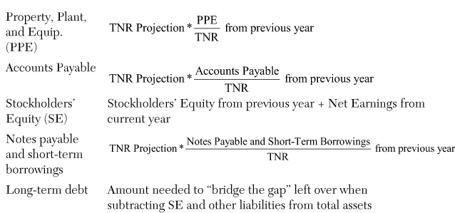
Thus far, we have calculated assets, shareholders’ equity, and some types of liabilities on the pro forma balance sheet. To calculate the remaining piece of the balance sheet (debt), we can expand the earlier equation:
Rearranging the equation, we find that

Therefore, we simply calculate debt as the difference between assets, shareholders’ equity, and the other liabilities that we have already included in the pro forma financial statement.
3.2.5.1 Debt
For the case of ABC, our 2014 balance sheet forecast shows total assets of $14.5 billion and stockholders’ equity of $6.3 billion. To calculate Other Liabilities, we need to sum up the nondebt pieces of the Liabilities section of the balance sheet. For ABC, these entries include accounts payable, employee compensation and benefits, taxes on earnings, deferred revenue, accrued restructuring, other accrued liabilities, and other liabilities. Taken together, these elements sum to $6.2 billion if we include short-term borrowings, and $5.5 billion if we do not include short-term borrowings. (We explain later the importance of this distinction.) Thus, assuming we include short-term borrowings in Other Liabilities, we can calculate the projected financial shortfall as $2.0 billion by subtracting shareholders’ equity and other liabilities from total assets. So, ABC needs to borrow $2 billion in total in the first year (2014) to sustain the pace of growth we are projecting. Intuitively, this calculation follows directly from the most basic rule about financial statements: that balance sheets must balance.
One additional complication is that there are several ways to borrow funds. In the case of ABC, one account on the balance sheet is “Notes payable and short-term borrowings” and another is “Long-term debt.” The needed debt could fall into either category. For the purposes of the exercise here, we assumed that short-term borrowings continue at the same percent of total net revenue as in 2013, implying that short-term debt in 2014 will be in the amount of $741 million. (This number is calculated by multiplying the ratio for short-term borrowings to net revenue that we have assumed for our forecast [6.35%] by our projected level of net revenue for 2014 [$11.7 billion].) Subtracting this amount of short-term debt from the amount of total debt needed, as we did earlier by including short-term with other liabilities, will give us the amount of long-term debt needed to finance this project. Based on our growth projection, ABC’s projected long-term debt for 2014 is about $2 billion. Essentially, long-term debt bridges the gap between assets and equity plus other liabilities (in this case, including short-term debt).
3.2.5.2 Interest Expenses
Now that we know the magnitude of debt, we can calculate the “Interest and other, net” category in the income statement. To do so, we simply multiply the interest rate in the Rates section in Figure 3.1.2 of our pro forma worksheet (2.27%) by the magnitude of both short-term and long-term debt. Doing so, we can see that interest costs are estimated to run to $62 million for 2014.
As a final point here, note that there is an inherent circularity to generating projections of interest expenses. To calculate 2014 interest expenses, we need to know 2014 levels of short-term and long-term debt. However, as noted earlier
However, to calculate debt, we must know interest expenses because interest expenses are used to calculate net earnings, which in turn flow into shareholders’ equity. (See Section 2.4, “Market Value Balance Sheets,” where we assumed that net earnings from a given year flow directly into equity for that year.) Thus, debt (because it is calculated using shareholders’ equity) and interest expenses must be simultaneously calculated. There are methods that can be used to make these calculations.1 An alternative way of generating an estimate for interest expenses is to take the debt level from the previous year (2013, in this case) and multiplying this debt level by the assumed interest rate. (For ABC, this would give us approximately: $2.5 billion * 2.27% = $58 million.) In reality, interest expenses are generated by the level of debt throughout the year, rather than by the level of debt at either the beginning (as shown, in this case, by the 2013 balance sheet) or end of the year (as shown, in this case, by the 2014 balance sheet). Therefore, this alternative approach is also reasonable.
3.3 Bridging Financial Shortfalls
Earlier, we assumed that the funding needed for expansion (that is, the financial shortfall) would come from debt. The gap between assets and other liabilities plus shareholders’ equity was bridged by borrowing. In reality, there are other ways to acquire funding. For example, a firm could issue equity, which would also bring in cash. Issuing equity has the downside of diluting the value of existing shares, but it also allows the firm to avoid future interest and principal payments. Alternatively, a firm could potentially sell some nonessential assets to generate funding.
An additional point to keep in mind is that the method that a firm uses to fund growth and the magnitude of the funding required are critical measures of whether a growth target is realistic. If the financial projection shows that a firm will be increasing borrowing every year into the foreseeable future, the firm likely will not be able to maintain the planned pace of expansion. We return to this point later in the chapter.
3.4 Financial Ratios
Figure 3.1.3 of the pro forma worksheet shows a number of the ratios introduced in Chapter 2. We can use the path over time of these ratios to evaluate a given growth path. Before evaluating the path, however, a firm needs to think about its goals for the future. Does it want to increase return on equity? By how much? How much debt is it willing to take on? After these decisions are made, ratio analysis shows the impact of a given growth strategy.
3.4.1 Performance Ratios
The first three ratios in Figure 3.1.3 provide information about a firm’s overall performance. Return on equity (ROE), return on assets (ROA), and profit margin all show the degree to which the firm is generating returns to investors. At the most basic level, a plan for growth should generate ROE, ROA, and a profit margin at least comparable to industry peers. If the plan does not generate growth at that level, it suggests that the plan is likely not worth pursuing and that obtaining financing for the plan is likely to be difficult.
We see that ABC had an ROE of 11% in 2013; our plans for 10% growth per year indicate an ROE that is around 10% in the first year, and then stays fairly flat throughout the forecast, ending up at around 10% ROE in 2018. The ROA is projected to remain fairly flat at around 4.5%. Therefore, this growth path essentially keeps the firm at around the same performance level as it had in 2013. For investors looking for stability, this plan may be attractive; however, it does not promise greater returns through the forecast period.
3.4.2 Leverage Ratios
One important decision variable for a path of growth is the degree to which a firm takes on debt. The leverage ratios show the extent to which expansion needs to be financed by borrowing. The leverage ratio shows the ratio of total borrowings to asset; a growing leverage ratio may be a cause for concern, a point that we return to in the next section. Our growth path for ABC shows a gradual decline in leverage, with a leverage ratio of 19% in 2014 steadily decreasing to 17% in 2018. From the leverage perspective, this growth path does not appear to raise any concerns.
The interest coverage, or net earnings before taxes minus interest expense divided by interest expense (see Figure 2.7), provides an indication of whether the firm will be able to handle any increased leverage associated with a growth plan. For ABC, the interest coverage ratio increases over the horizon of the forecast, growing from 14 in 2014 to 16 in 2018. Because an increasing ratio implies that income available to pay interest expenses will rise relative to those interest payments, this path for interest coverage indicates that covering interest payments would become increasingly less burdensome over the course of the forecast. Again, this ratio does not raise any red flags about the feasibility of this projected growth path.
3.5 Sustainable Growth
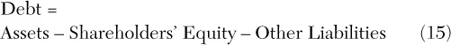
We can think about the sustainable level of growth in two ways. First, in the long run, a firm will not be able to grow at a faster pace than the rate of growth in returns to equity. Recall the expression we used earlier:
Assets = Liabilities + Shareholders’ Equity
Assets = Debt + Other Liabilities + Shareholders’ Equity
Shareholders’ Equity = Assets – Debt – Other Liabilities
This relationship is also illustrated in Figure 3.2. In the example in the figure, we assume that sales grow at 10%. Based on our assumptions about growth in assets (and also nondebt liabilities), this means that either debt or stockholders’ equity must grow to match the expansion in the right side of the balance sheet. A firm would not be able to maintain a constant increase in debt with no end in sight for borrowing, because a lender would not be willing to extend funds indefinitely. To maintain a certain level of growth in assets, therefore, a firm must grow at a pace no greater than the growth rate of the return on equity, because this number represents the increase in the shareholders’ equity portion of the balance sheet. In other words
Maximum Sustainable Growth Rate = Return on Equity
In Figure 3.2, the ROE must be at least 10% for that pace of growth to be sustainable.
An alternative way to think about the sustainable level of growth is to focus on the leverage ratio. A leverage ratio that increases each year of a forecast raises red flags about whether the planned path is actually feasible. A constantly increasing debt ratio indicates that a firm’s growth is based on higher and higher debt as a percent of assets. In other words, debt is increasing faster than assets. This path would not be feasible as a long-term path.
Returning to Figure 3.1, we can analyze whether our proposed growth path for ABC is sustainable. The ratios in Figure 3.1.3 show, first, that the projected ROE hovers around 10% over the five-year projection. With ROE around the same level as the planned growth in revenue, this path does appear sustainable, and does not raise any obvious concerns, just as we concluded in our earlier discussion of the declining leverage ratio and the increasing interest coverage. Thus, both of these approaches indicate that our planned growth of 10% per year is sustainable, although it is below the maximum sustainable growth rate.
Endnote
1. If these calculations are made using Microsoft Excel, Excel Calculation Preferences must be set to Limit Iterations. If this setting is different, an error message will result stating that Excel is not able to calculate the formula because it contains a circular reference.