5
Monte Carlo Simulations (Nonthermal)
Unit I of this chapter addresses the problem of how computers generate numbers that appear random and how we can determine how random they are. Unit II shows how to use these random numbers to simulate physical processes. In Chapter 6, “Integration,” we see show how to use these random numbers to evaluate integrals, and in Chapter 15, “Thermodynamic Simulations & Feynman Quantum Path Integration,” we investigate the use of random numbers to simulate thermal processes and the fluctuations in quantum systems.
5.1 Unit I. Deterministic Randomness
Some people are attracted to computing because of its deterministic nature; it’s nice to have a place in one’s life where nothing is left to chance. Barring machine errors or undefined variables, you get the same output every time you feed your program the same input. Nevertheless, many computer cycles are used for Monte Carlo calculations that at their very core include elements of chance. These are calculations in which random numbers generated by the computer are used to simulate naturally random processes, such as thermal motion or radioactive decay, or to solve equations on the average. Indeed, much of computational physics’ recognition has come about from the ability of computers to solve previously intractable problems using Monte Carlo techniques.
5.2 Random Sequences (Theory)
We define a sequence of numbers r1,r2,… as random if there are no correlations among the numbers. Yet being random does not mean that all the numbers in the sequence are equally likely to occur. If all the numbers in a sequence are equally likely to occur, then the sequence is said to be uniform, and the numbers can be random as well. To illustrate, 1, 2, 3, 4,. .. is uniform but probably not random. Further,it is possible to have a sequence of numbers that, in some sense, are random but have very short-range correlations among themselves, for example,
have short-range but not long-range correlations.
Mathematically, the likelihood of a number occurring is described by a distribution function P(r), where P(r) dr is the probability of finding r in the interval [r, r +dr]. A uniform distribution means that P(r) = a constant. The standard random-number generator on computers generates uniform distributions between 0 and 1. In other words, the standard random-number generator outputs numbers in this interval, each with an equal probability yet each independent of the previous number. As we shall see, numbers can also be generated nonuniformly and still be random.
By the nature of their construction, computers are deterministic and so cannot create a random sequence. By the nature of their creation, computed random number sequences must contain correlations and in this way are not truly random. Although it may be a bit of work, if we know rm and its preceding elements, it is always possible to figure out rm+1. For this reason, computers are said to generate pseudorandom numbers (yet with our incurable laziness we won’t bother saying “pseudo” all the time). While more sophisticated generators do a better job at hiding the correlations, experience shows that if you look hard enough or use these numbers long enough, you will notice correlations. A primitive alternative to generating random numbers is to read in a table of true random numbers determined by naturally random processes such as radioactive decay or to connect the computer to an experimental device that measures random events. This alternative is not good for production work but may be a useful check in times of doubt.
5.2.1 Random-Number Generation (Algorithm)
The linear congruent or power residue method is the common way of generating a pseudorandom sequence of numbers 0 ≤ ri ≤ M -1 over the interval [0,M -1]. You multiply the previous random numberri-1 by the constanta, add another constant c, take the modulus by M, and then keep just the fractional part (remainder)1 as the next random number ri+1:
The value for r1 (the seed) is frequently supplied by the user, and mod is a built-in function on your computer for remaindering (it may be called amod or dmod). This is essentially a bit-shift operation that ends up with the least significant part of the input number and thus counts on the randomness of round-off errors to generate a random sequence.
As an example, if c = 1,a = 4,M = 9, and you supply r1 = 3, then you obtain the sequence
![]()

Figure 5.1 Left: A plot of successive random numbers (x, y) = (ri,ri+1) generated with a deliberately“bad” generator. Right: A plot generated with the library routine drand48.

We get a sequence of length M = 9, after which the entire sequence repeats. If we want numbers in the range [0,1], we divide the r’s by M = 9:
![]()
This is still a sequence of length 9 but is no longer a sequence of integers. If random numbers in the range [A, B] are needed, you only need to scale:
![]()
As a rule of thumb: Before using a random-number generator in your programs, you should check its range and that it produces numbers that “look” random.
Although not a mathematical test, you should always make a graphical display of your random numbers.Your visual cortex is quite refined at recognizing patterns and will tell you immediately if there is one in your random numbers. For instance, Figure 5.1 shows generated sequences from “good” and “bad” generators, and it is clear which is not random (although if you look hard enough at the random points, your mind may well pick out patterns there too).
The linear congruent method (5.1) produces integers in the range [0,M — 1] and therefore becomes completely correlated if a particular integer comes up a second time (the whole cycle then repeats). In order to obtain a longer sequence, a and M should be large numbers but not so large that ar¿_1 overflows. On a computer using 48-bit integer arithmetic, the built-in random-number generator may use M values as large as 248 3 × 10¹⁴. A 32-bit generator may use M = 231 ~2x 10⁹. If your program uses approximately this many random numbers, you may need to reseed the sequence during intermediate steps to avoid the cycle repeating.
Your computer probably has random-number generators that are better than the one you will compute with the power residue method. You may check this out in the manual or the help pages (try the man command in Unix) and then test the generated sequence. These routines may have names like rand, rn, random, srand, erand, drand, or drand48.
We recommend a version of drand48 as a random-number generator. It generates random numbers in the range [0,1] with good spectral properties by using 48-bit integer arithmetic with the parameters2

To initialize the random sequence, you need to plant a seed in it. In Fortran you call the subroutine srand48 to plant your seed, while in Java you issue the statement Random randnum = new Random(seed); (see RandNum.java in Listing 5.1 for details).

Listing 5.1 RandNum.java calls the random-number generator from the Java utility class. Note that a different seed is needed for a different sequence.

Figure 5.2 A plot of a uniform pseudorandom sequence ri versus i. The points are connected to make it easier to follow the order.
5.2.2 Implementation: Random Sequence
1. Write a simple program to generate random numbers using the linear congruent method (5.1).
2. For pedagogical purposes, try the unwise choice: (a, c, M, r1) = (57, 1, 256,10). Determine the period, that is, how many numbers are generated before the sequence repeats.
3. Take the pedagogical sequence of random numbers and look for correlations by observing clustering on a plot of successive pairs (xi, yi) = (r2i-1, r2i), i = 1, 2,…. (Do not connect the points with lines.) You may “see” correlations (Figure 5.1), which means that you should not use this sequence for serious work.
4. Make your own version of Figure 5.2; that is, plot ri versus i.
5. Test the built-in random-number generator on your computer for correlations by plotting the same pairs as above. (This should be good for serious work.)
6. Test the linear congruent method again with reasonable constants like those in (5.8) and (5.9). Compare the scatterplot you obtain with that of the built-in random-number generator. (This, too, should be good for serious work.)
![]()
TABLE 5.1
A Table of a Uniform Pseudorandom Sequence ri Generated by RandNum.java

For scientific work we recommend using an industrial-strength random-number generator. To see why, here we assess how bad a careless application of the power residue method can be.
5.2.3 Assessing Randomness and Uniformity
Because the computer’s random numbers are generated according to a definite rule, the numbers in the sequence must be correlated with each other. This can affect a simulation that assumes random events. Therefore it is wise for you to test a random-number generator to obtain a numerical measure of its uniformity and randomness before you stake your scientific reputation on it. In fact, some tests are simple enough for you to make it a habit to run them simultaneously with your simulation. In the examples to follow, we test for either randomness or uniformity.
1. Probably the most obvious, but often neglected, test for randomness and uniformity is to look at the numbers generated. For example, Table 5.1 presents some output from RandNum.java. If you just look at these numbers, you will know immediately that they all lie between 0 and 1, that they appear to differ from each other, and that there is no obvious pattern (like 0.3333).
2. As we have seen, a quick visual test (Figure 5.2) involves taking this same list and plotting it with ri as ordinate and i asabscissa.Observehow there appears to be a uniform distribution between 0 and 1 and no particular correlation between points (although your eye and brain will try to recognize some kind of pattern).
3. A simple test of uniformity evaluates the kth moment of a distribution:
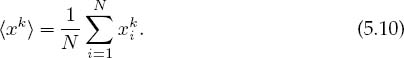
If the numbers are distributed uniformly, then (5.10) is approximately the moment of the distribution function P(x):

If (5.11) holds for your generator, then you know that the distribution is uni-√ form. If the deviation from (5.11) varies as 1/ N, then you also know that the distribution is random.
4. Another simple test determines the near-neighbor correlation in your random sequence by taking sums of products for small k:

If your random numbersxi andxi+k are distributed with the joint probability distribution P(xi,xi+k) and are independent and uniform, then (5.12) can be approximated as an integral:

If (5.13)holds for your random numbers,then you know that they are uniform and independent. If the deviation from (5.13) varies as 1/ N, then you also know that the distribution is random.
5. As we have seen, an effective test for randomness is performed by making a scatterplot of (xi = r2i, yi = r2i+1) for many i values. If your points have noticeable regularity, the sequence is not random. If the points are random, they should uniformly fill a square with no discernible pattern(a cloud) (Figure 5.1).
6. Test your random-number generator with (5.11) for k = 1,3,7 and N = 100, 10, 000, 100,000. In each case print out

to check that it is of order 1.
![]()
5.3 Unit II. Monte Carlo Applications
Now that we have an idea of how to use the computer to generate pseudorandom numbers, we build some confidence that we can use these numbers to incorporate the element of chance into a simulation. We do this first by simulating a random walk and then by simulating an atom decaying spontaneously. After that, we show how knowing the statistics of random numbers leads to the best way to evaluate multidimensional integrals.
5.4 A Random Walk (Problem)
Consider a perfume molecule released in the front of a classroom. It collides randomly with other molecules in the air and eventually reaches your nose even though you are hidden in the last row. The problem is to determine how many collisions, on the average, a perfume molecule makes in traveling a distance R. You are given the fact that a molecule travels an average (root-mean-square) distance rrms between collisions.
5.4.1 Random-Walk Simulation
There are a number of ways to simulate a random walk with (surprise, surprise) different assumptions yielding different physics. We will present the simplest approach for a 2-D walk, with a minimum of theory, and end up with a model for normal diffusion. The research literature is full of discussions of various versions of this problem. For example, Brownian motion corresponds to the limit in which the individual step lengths approach zero with no time delay between steps. Additional refinements include collisions within a moving medium (abnormal diffusion), including the velocities of the particles, or even pausing between steps. Models such as these are discussed in Chapter 13, “Fractals & Statistical Growth,” and demonstrated by some of the corresponding applets on the CD (available online: http://press.princeton.edu/landau_survey/).
![]()
In our random-walk simulation (Figure 5.3) an artificial walker takes sequential steps with the direction of each step independent of the direction of the previous step. For our model we start at the origin and take N steps in the xy plane of lengths (not coordinates)
Even though each step may be in a different direction, the distances along each Cartesian axis just add algebraically (aren’t vectors great?). Accordingly, the radial distance R from the starting point after N steps is


Figure 5.3 Some of the N steps in a random walk that end up a distance R from the origin. Notice how the Δx’s for each step add algebraically.
If the walk is random, the particle is equally likely to travel in any direction at each step. If we take the average of a large number of such random steps, all the cross terms in (5.16) will vanish and we will be left with

where rrms = J’(r2) is the root-mean-square step size.
To summarize, if the walk is random, then we expect that after a large number of steps the average vector distance from the origin will vanish:
![]()
However, (5.17) indicates that the average scalar distance from the origin is Nrrms, where each step is of average length rrms. In other words, the vector endpoint will be distributed uniformly in all quadrants, and so the displacement vector averages to zero, but the length of that vector does not. For large N values, Nr rms <C Nr rms but does not vanish. In our experience, practical simulations agree with this theory, but rarely perfectly, with the level of agreement depending upon the details of how the averages are taken and how the randomness is built into each step.
5.4.2 Implementation: Random Walk
The program Walk.java on the instructor’s CD (available online: http://press.princeton.edu/landau_survey/) is our random-walk simulation. It’s key element is random values for the x and y components of each step,


Figure 5.4 Left: A computer simulation of a random walk. Right: The distance covered in two simulated walks of N steps using different schemes for including randomness. The theoretical prediction (5.17) is the straight line.
Here we omit the scaling factor that normalizes each step to length 1. When using your computer to simulate a random walk, you should expect to obtain (5.17) only as the average displacement after many trials, not necessarily as the answer for each trial. You may get different answers depending on how you take your random steps (Figure 5.4 right).
Start at the origin and take a 2-D random walk with your computer.
1. To increase the amount of randomness, independently choose random values for Δx’ and Δy’ in the range [—1,1]. Then normalize them so that each step is of unit length

2. Use a plotting program to draw maps of several independent random walks, each of 1000 steps. Comment on whether these look like what you would expect of a random walk.
3. If you have your walker taking N steps in a single trial, then conduct a total number K ^/N of trials. Each trial should have N steps and start with a different seed.
4. Calculate the mean square distance R2 for each trial and then take the average of R2 for all your K trials:

5. Check the validity of the assumptions made in deriving the theoretical result (5.17) by checking how well
Do your checking for both a single (long) run and for the average over trials.
6. Plot the root-mean-square distance Rrms = ^/(R2(N)) as a function of yN. Values of N should start with a small number, where R N is not expected to be accurate, and end at a quite large value, where two or three places of accuracy should be expected on the average.
![]()
5.5 Radioactive Decay (Problem)
Your problem is to simulate how a small number N of radioactive particles decay3 In particular, you are to determine when radioactive decay looks like exponential decay and when it looks stochastic (containing elements of chance). Because the exponential decay law is a large-number approximation to a natural process that always ends with small numbers, our simulation should be closer to nature than is the exponential decay law (Figure 5.5). In fact, if you go to the CD (available online: http://press.princeton.edu/landau_survey/) and “listen” to the output of the decay simulation code, what you will hear sounds very much like a Geiger counter, a convincing demonstration of the realism of the simulation.
![]()
Spontaneous decay is a natural process in which a particle, with no external stimulation, decays into other particles. Even though the probability of decay of any one particle in any time interval is constant, just when it decays is a random event. Because the exact moment when any one particle decays is random, it does not matter how long the particle has been around or whether some other particles have decayed. In other words, the probability P of any one particle decaying per unit time interval is a constant, and when that particle decays, it is gone forever. Of course, as the total number of particles decreases with time, so will the number of decays, but the probability of any one particle decaying in some time interval is always the same constant as long as that particle exists.
5.5.1 Discrete Decay (Model)
Imagine having a sample of N(t) radioactive nuclei at time t (Figure 5.5 inset). Let ΔN be the number of particles that decay in some small time interval Δ t. We convert the statement “the probability P of any one particle decaying per unit time is a constant” into the equation

Figure 5.5 A sample containing N nuclei, each one of which has the same probability of decaying per unit time (circle). Semilog plots of the results from several decay simulations. Notice how the decay appears exponential (like a straight line) when the number of nuclei is large, but stochastic for log N ≤ 2.0.

where the constant λ is called the decay rate. Of course the real decay rate or activity is ΔN(t)/ Δt, which varies with time. In fact, because the total activity is proportional to the total number of particles still present, it too is stochastic with an exponential-like decay in time. [Actually, because the number of decays ΔN(t) is proportional to the difference in random numbers, its stochastic nature becomes evident before that of N(t).]
Equation (5.20) is a finite-difference equation in terms of the experimental measurables N(t), ΔN(t), and Δ t. Although it cannot be integrated the way a differential equation can, it can be solved numerically when we include the fact that the decay process is random. Because the process is random, we cannot predict a single value for ΔN(t), although we can predict the average number of decays when observations are made of many identical systems of N decaying particles.
5.5.2 Continuous Decay (Model)
When the number of particles N —> ∞ and the observation time interval Δ t —> 0, an approximate form of the radioactive decay law (5.20) results:
![]()
This can be integrated to obtain the time dependence of the total number of particles and of the total activity:

We see that in this limit we obtain exponential decay, which leads to the identification of the decay rate λ with the inverse lifetime:
![]()
So we see from its derivation that exponential decay is a good description of nature for a large number of particles where ΔN/N ![]() 0. The basic law of nature (5.19) is always valid, but as we will see in the simulation, exponential decay (5.23) becomes less and less accurate as the number of particles becomes smaller and smaller.
0. The basic law of nature (5.19) is always valid, but as we will see in the simulation, exponential decay (5.23) becomes less and less accurate as the number of particles becomes smaller and smaller.
5.5.3 Decay Simulation
A program for simulating radioactive decay is surprisingly simple but not without its subtleties. We increase time in discrete steps of Δ t, and for each time interval we count the number of nuclei that have decayed during that Δ t. The simulation quits when there are no nuclei left to decay. Such being the case, we have an outer loop over the time steps Δ t and an inner loop over the remaining nuclei for each time step. The pseudocode is simple:

When we pick a value for the decay rate λ = 1/τ to use in our simulation, we are setting the scale for times. If the actual decay rate is λ = 0.3 × 10⁶ s-1 and if we decide to measure times in units of 10-6 s, then we will choose random numbers 0 < ri < 1, which leads to λ values lying someplace near the middle of the range (e.g., λ ![]() 0.3). Alternatively, we can use a value of λ = 0.3 × 10⁶ s-1 in our simulation and then scale the random numbers to the range 0 < ri < 106. However, unless you plan to compare your simulation to experimental data, you do not have to worry about the scale for time but instead should focus on the physics behind the slopes and relative magnitudes of the graphs.
0.3). Alternatively, we can use a value of λ = 0.3 × 10⁶ s-1 in our simulation and then scale the random numbers to the range 0 < ri < 106. However, unless you plan to compare your simulation to experimental data, you do not have to worry about the scale for time but instead should focus on the physics behind the slopes and relative magnitudes of the graphs.

Listing 5.2 Decay.java simulates spontaneous decay in which a decay occurs if a random number is smaller than the decay parameter.
5.6 Decay Implementation and Visualization
Write a program to simulate radioactive decay using the simple program in Listing 5.2 as a guide. You should obtain results like those in Figure 5.5.
1. Plot the logarithm of the number left lnN(t) and the logarithm of the decay rate ln ΔN(t) versus time. Note that the simulation measures time in steps of Δt (generation number).
2. Check that you obtain what looks like exponential decay when you start with large values for N(0), but that the decay displays its stochastic nature for small N(0) [large N(0) values are also stochastic; they just don’t look like it].
3. Create two plots, one showing that the slopes of N(t) versus t are independent of N(0) and another showing that the slopes are proportional to λ.
4. Create a plot showing that within the expected statistical variations, ln N(t) and ln ΔN(t) are proportional.
5. Explain in your own words how a process that is spontaneous and random at its very heart can lead to exponential decay.
6. How does your simulation show that the decay is exponential-like and not a power law such as N = βt-α?
![]()
1 You may obtain the same result for the modulus operation by subtracting M until any further subtractions would leave a negative number; what remains is the remainder.
2 Unless you know how to do 48-bit arithmetic and how to input numbers in different bases, it may be better to enter large numbers like M = 112233 and a = 9999.
3 Spontaneous decay is also discussed in Chapter 8, “Solving Systems of Equations with Matrices; Data Fitting,” where we fit an exponential function to a decay spectrum.