
20
Integral Equations in Quantum Mechanics
The power and accessibility of high-speed computers have changed the view as to what kind of equations are soluble. In Chapter 9, “Differential Equation Applications,” and Chapter 12, “Discrete & Continuous Nonlinear Dynamics,” we saw how even nonlinear differential equations can be solved easily and can give new insight into the physical world. In this chapter we examine how the integral equations of quantum mechanics can be solved for both bound and scattering states. In Unit I we extend our treatment of the eigenvalue problem, solved as a coordinate-space differential equation in Chapter 9, to the equivalent integral-equation problem in momentum space. In Unit II we treat the singular integral equations for scattering, a more difficult problem. After studying this chapter, we hope that the reader will view both integral and differential equations as soluble.
20.1 Unit I. Bound States of Nonlocal Potentials
Problem: A particle undergoes a many-body interaction with a medium (Figure 20.1) that results in the particle experiencing an effective potential at r that depends on the wave function at the r’ values of the other particles [L 96]:

This type of interaction is called nonlocal and leads to a Schrödinger equation that is a combined integral and differential (“integrodifferential”) equation:

Your problem is to figure out how to find the bound-state energies E and wave functions ψ for the integral equation in (20.2).1
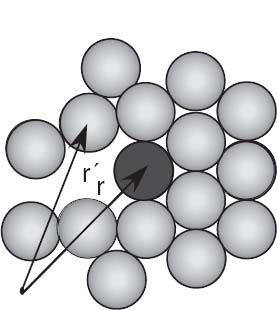
Figure 20.1 A dark particle moving in a dense multiparticle medium. The nonlocality of the potential felt by the dark particle at r arises from the particle interactions at all r’.
20.2 Momentum-Space Schrödinger Equation (Theory)
One way of dealing with equation (20.2) is by going to momentum space where it becomes the integral equation [L 96]

where we restrict our solution to l = 0 partial waves. In (20.3), V (k, p) is the momentum-space representation (double Fourier transform) of the potential,

and ψ(k) is the (unnormalized) momentum-space wave function (the probability amplitude for finding the particle with momentum k),

Equation (20.3) is an integral equation for ψ(k), in contrast to an integral representation of ψ(k), because the integral in it cannot be evaluated until ψ(p) is known. Although this may seem like an insurmountable barrier, we will transform this equation into a matrix equation that can be solved with the matrix techniques discussedin Chapter8,“ Solving Systems of Equations with Matrices; Data Fitting.”

Figure 20.2 The grid of momentum values on which the integral equation is solved.
20.2.1 Integral to Linear Equations (Method)
We approximate the integral over the potential as a weighted sum over N integration points (usually Gauss quadrature2) for p = kj, j = 1,N:

This converts the integral equation (20.3) to the algebraic equation

Equation (20.7) contains the N unknowns ψ(kj), the single unknown E, and the unknown function ψ(k). We eliminate the need to know the entire function ψ(k) by restricting the solution to the same values of ki as used to approximate the integral. This leads to a set of N coupled linear equations in (N +1) unknowns:

As a case in point, if N = 2, we would have the two simultaneous linear equations

We write our coupled dynamic equations in matrix form as

or as explicit matrices

Equation (20.9) is the matrix representation of the Schrödinger equation (20.3). The wave function ψ(k) on the grid is the N ×1 vector

The astute reader may be questioning the possibility of solving N equations for (N +1)unknowns. That reader is wise; only sometimes, and only for certain values of E (eigenvalues) will the computer be able to find solutions. To see how this arises, we try to apply the matrix inversion technique (which we will use successfully for scattering in Unit II). We rewrite (20.9) as
![]()
and multiply both sides by the inverse of [H -EI] to obtain the formal solution
![]()
This equation tells us that (1) if the inverse exists, then we have the trivial solution ψ ≡ 0, which is not very interesting, and (2) for a nontrivial solution to exist, our assumption that the inverse exists must be incorrect. Yet we know from the theory of linear equations that the inverse fails to exist when the determinant vanishes:
![]()
Equation (20.14) is the additional equation needed to find unique solutions to the eigenvalue problem. Nevertheless, there is no guarantee that solutions of (20.14) can always be found, but if they are found, they are the desired eigenvalues of (20.9).
20.2.2 Delta-Shell Potential (Model)
To keep things simple and tohavean analytic answer to compare with,weconsider the local delta-shell potential:

This would be a good model for an interaction that occurs in 3-D when two particles are predominantly a fixed distance b apart. We use (20.4) to determine its momentum-space representation:

Beware: We have chosen this potential because it is easy to evaluate the momentum-space matrix element of the potential. However, its singular nature in r space leads to a very slow falloff in k space, and this causes the integrals to converge so slowly that numerics are not as precise as we would like.
If the energy is parameterized in terms of a wave vector κ by E = -κ2/2µ, then for this potential there is, at most, one bound state and it satisfies the transcendental equation [Gott 66]
![]()
Note that bound states occur only for attractive potentials and only if the attraction is strong enough. For the present case this means that we must have λ < 0.
Exercise: Pick some values of b and λ and use them to verify with a hand calculation that (20.17) can be solved for κ.
20.2.3 Binding Energies Implementation
An actual computation may follow two paths. The first calls subroutines to evaluate the determinant of the [H – EI] matrix in (20.14) and then to search for those values of energy for which the computed determinant vanishes. This provides E, but not wave functions. The other approach calls an eigenproblem solver that may give some or all eigenvalues and eigenfunctions. In both cases the solution is obtained iteratively, and you may be required to guess starting values for both the eigenvalues and eigenvectors. In Listing 20.1 we present our solution of the integral equation for bound states of the delta-shell potential using the JAMA matrix library and the gauss method for Gaussian quadrature points and weights.

Listing 20.1 Bound.java solves the Lippmann–Schwinger integral equation for bound states within a delta-shell potential. The integral equations are converted to matrix equations using Gaussian grid points, and they are solved with JAMA.
1. Write your own program, or modify the code on the CD http://press.princeton.edu/landau_survey/), to solve the integral equation (20.9) for the delta-shell potential (20.16). Either evaluate the determinant of [H – EI] and then find the E for which the determinant vanishes or find the eigenvalues and eigenvectors for this H.
2. Set the scale by setting 2µ = 1 and b = 10.
3. Set up the potential and Hamiltonian matrices V (i, j)and H(i, j)for Gaussian quadrature integration with at least N = 16 grid points.
4. Adjust the value and sign of λ for bound states. A good approach is to start with a large negative value for λ and then make it less negative. You should find that the eigenvalue moves up in energy.
5. Try increasing the number of grid points in steps of 8, for example, 16, 24, 32, 64, …, and see how the energy changes.
6. Note: Your eigenenergy solver may return several eigenenergies. The true bound state will be at negative energy and will be stable as the number of grid points changes. The others are numerical artifacts.
7. Extract the best value for the bound-state energy and estimate its precision by seeing how it changes with the number of grid points.
8. Check your solution by comparing the RHS and LHS in the matrix multiplication [H][ψ] = E[ψ].
9. Verify that, regardless of the potential’s strength, there is only a single bound state and that it gets deeper as the magnitude of λ increases.
![]()
20.2.4 Wave Function (Exploration)
1. Determine the momentum-space wave function ψ(k). Does it fall off at k → ∞? Does it oscillate? Is it well behaved at the origin?
2. Determine the coordinate-space wave function via the Bessel transform

Does ψ0(r) fall off as you would expect for a bound state? Does it oscillate? Is it well behaved at the origin?
2. 3. Compare the r dependence of this ψ0(r) to the analytic wave function:
![]()

20.3 Unit II. Nonlocal Potential Scattering 
Problem: Again we have a particle interacting with the nonlocal potential discussed in Unit I (Figure 20.3 left), only now the particle has sufficiently high energy that it scatters rather than binds with the medium. Your problem is to determine the scattering cross section for scattering from a nonlocal potential.

Figure 20.3 Left: A projectile of momentum k (dark particle at r) scattering from a dense medium. Right: The same process viewed in the CM system, where the k’s are CM momenta.
20.4 Lippmann–Schwinger Equation (Theory)
Because experiments measure scattering amplitudes and not wave functions, it is more direct to have a theory dealing with amplitudes rather than wave functions. An integral form of the Schrödinger equation dealing with the reaction amplitude or R matrix is the Lippmann–Schwinger equation:

As in Unit I, the equations are for partial wave l = 0 and h=1. In (20.20) the momentum ko is related to the energy E and the reduced mass µ by

and the initial and final COM momenta k and k’ are the momentum-space variables. The experimental observable that results from a solution of (20.20) is the diagonal matrix element R(ko, k), which is related to the scattering phase shift δQ and thus the cross section:
![]()
Note that (20.20) is not just the evaluation of an integral; it is an integral equation in which R(p, k) is integrated over all p, yet since R(p, k) is unknown, the integral cannot be evaluated until after the equation is solved! The symbol P in (20.20) indicates the Cauchy principal-value prescription for avoiding the singularity arising from the zero of the denominator (we discuss how to do that next).

Figure 20.4 Three different paths in the complex k’ plane used to evaluate line integrals when there are singularities. Here the singularities are at k and -k, and the integration variable is k’.
20.4.1 Singular Integrals (Math)
A singular integral

is one in which the integrand g(k) is singular at a point k0 within the interval [a, b] and yet the integral G is still finite. (If the integral itself were infinite, we could not compute it.) Unfortunately, computers are notoriously bad at dealing with infinite numbers, and if an integration point gets too near the singularity, overwhelming subtractive cancellation or overflow may occur. Consequently, we apply some results from complex analysis before evaluating singular integrals numerically.3
In Figure 20.4 we show three ways in which the singularity of an integrand can be avoided. The paths in Figures 20.4A and 20.4B move the singularity slightly off the real k axis by giving the singularity a small imaginary part ±iε. The Cauchy principal-value prescription P (Figure 20.4C) is seen to follow a path that “pinches” both sides of the singularity at ko but does not to pass through it:

The preceding three prescriptions are related by the identity
![]()
which follows from Cauchy’s residue theorem.
20.4.2 Numerical Principal Values
A numerical evaluation of the principal value limit (20.24) is awkward because computers have limited precision. A better algorithm follows from the theorem

This equation says that the curve of 1/(k -k0) as a function of k has equal and opposite areas on both sides of the singular point k0. If we break the integral up into one over positive k and one over negative k, a change of variable k → −k permits us to rewrite (20.26) as

We observe that the principal-value exclusion of the singular point’s contribution to the integral is equivalent to a simple subtraction of the zero integral (20.27):

Notice that there is no P on the RHS of (20.28) because the integrand is no longer singular at k = k0 (it is proportional to the df/dk) and can therefore be evaluated numerically using the usual rules. The integral (20.28) is called the Hilbert transform of f and also arises in inverse problems.
20.4.3 Reducing Integral Equations to Matrix Equations (Algorithm)
Now that we can handle singular integrals, we can go about reducing the integral equation (20.20) to a set of linear equations that can be solved with matrix methods. We start by rewriting the principal-value prescription as a definite integral [H&T 70]:

We convert this integral equation to linear equations by approximating the integral as a sum over N integration points (usually Gaussian) kj with weights wj:

We note that the last term in (20.30) implements the principal-value prescription and cancels the singular behavior of the previous term. Equation (20.30) contains the (N +1) unknowns R(kj,k0) for j = 0,N. We turn it into (N +1) simultaneous equations by evaluating it for (N + 1) k values on a grid (Figure 20.2) consisting of the observable momentum k0 and the integration points:

There are now (N +1) linear equations for (N +1) unknowns Ri ≡ R(ki,k0):

We express these equations in matrix form by combining the denominators and weights into a single denominator vector D:

The linear equations (20.32) now assume that the matrix form
![]()
where R and V are column vectors of length N + 1:

We call the matrix [1-DV ] in (20.34) the wave matrix F and write the integral equation as the matrix equation
![]()
With R the unknown vector, (20.36) is in the standard form AX = B, which can be solved by the mathematical subroutine libraries discussed in Chapter 8, “Solving Systems of Equations with Matrices; Data Fitting.”
20.4.4 Solution via Inversion or Elimination
An elegant (but alas not efficient) solution to (20.36) is by matrix inversion:
![]()

Listing 20.2 Scatt.java solves the Lippmann–Schwinger integral equation for scattering from a delta-shell potential. The singular integral equations are regularized by a subtraction, converted to matrix equations using Gaussian grid points,and then solved with JAMA.
Because the inversion of even complex matrices is a standard routine in mathematical libraries, (20.37) is a direct solution for the R matrix. Unless you need the inverse for other purposes (like calculating wave functions), a more efficient approach is to use Gaussian elimination to find an [R] that solves [F][R] = [V] without computing the inverse.
20.4.5 Scattering Implementation
For the scattering problem, we use the same delta-shell potential (20.16) discussed in §20.2.2 for bound states:
This is one of the few potentials for which the Lippmann–Schwinger equation (20.20) has an analytic solution [Gott 66] with which to check:
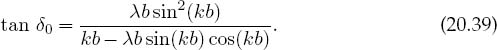
Our results were obtained with 2µ = 1, λb = 15, and b = 10, the same as in [Gott 66]. In Figure 20.5 we give a plot of sin δ0 versus kb, which is proportional to the scattering cross section arising from the l = 0 phase shift. It is seen to reach its maximum values at energies corresponding to resonances. In Listing 20.2 we present our program for solving the scattering integral equation using the JAMA matrix library and the gauss method for quadrature points. For your implementation:
1. Set up the matrices V[], D[], and F[][].Use at least N = 16 Gaussian quadrature points for your grid.
2. Calculate the matrix F-1 using a library subroutine.
3. Calculate the vector R by matrix multiplication R = F-1V.
4. Deduce the phase shift δ from the i = 0 element of R:
![]()
5. Estimate the precision of your solution by increasing the number of grid point in steps of two (we found the best answer for N = 26). If your phase shift changes in the second or third decimal place, you probably have that much precision.
6. Plot sin2 δ versus energy E = k 02/2µ starting at zero energy and ending at energies where the phase shift is again small. Your results should be similar to those in Figure 20.5. Note that a resonance occurs when δι increases rapidly through π/2, that is, when sin δ 0 = 1.
7. Check your answer against the analytic results (20.39).
![]()

Figure 20.5 The energy dependence of the cross section for l = 0 scattering from an attractive delta-shell potential with λ b = 15. The dashed curve is the analytic solution (20.39), and the solid curve results from numerically solving the integral Schrödinger equation, either via direct matrix inversion or via LU decomposition.
20.4.6 Scattering Wave Function (Exploration)
1. The F-1 matrix that occurred in our solution to the integral equation

is actually quite useful. In scattering theory it is known as the wave matrix because it is used in expansion of the wave function:
![]()
Here N0 is a normalization constant and the R matrix gives standing-wave boundary conditions. Plot u(r) and compare it to a free wave.
![]()
1 We use natural units in which ¯h ≡ 1 and omit the traditional bound-state subscript n on E and ψ in order to keep the notation simpler.
2 See Chapter 6, “Integration,” for a discussion of numerical integration.
3 [S&T 93] describe a different approach using Maple and Mathematica.