15

Thermodynamic Simulations & Feynman Quantum Path Integration

In Unit I of this chapter we describe how magnetic materials are simulated by using the Metropolis algorithm to solve the Ising model. This extends the techniques studied in Chapter 5, “Monte Carlo Simulations,” to thermodynamics. Not only do thermo-dynamic simulations have important practical applications, but they also give us insight into what is “dynamic” in thermodynamics. In Unit II we describe a new Monte Carlo algorithm known as Wang–Landau sampling that in the last few years has shown itself to be far more efficient than the 50-year-old Metropolis algorithm. Wang–Landau sampling is an active subject in present research, and it is nice to see it fitting well into an elementary textbook. Unit III applies the Metropolis algorithm to Feynman’s path integral formulation of quantum mechanics [F&H 65]. The theory, while the most advanced to be found in this book, forms the basis for field-theoretic calculations of quantum chromodynamics, some of the most fundamental and most time-consuming computations in existence. Basic discussions can be found in [Mann 83, MacK 85, M&N 87], with a recent review in [Potv 93].

15.1 Unit I. Magnets via the Metropolis Algorithm

Ferromagnets contain finite-size domains in which the spins of all the atoms point in the same direction. When an external magnetic field is applied to these materials, the different domains align and the materials become “magnetized.” Yet as the temperature is raised, the total magnetism decreases, and at the Curie temperature the system goes through a phasetransition beyond which all magnetizationvanishes. Your problem is to explain the thermal behavior of ferromagnets.

15.2 An Ising Chain (Model)

As our model we consider N magnetic dipoles fixed in place on the links of a linear chain (Figure 15.1). (It is a straightforward generalization to handle 2-D and 3-D lattices.) Because the particles are fixed, their positions and momenta are not dynamic variables, and we need worry only about their spins. We assume that the particle at site i has spin s_i, which is either up or down:

Figure 15.1 A 1-D lattice of N spins. The interaction energy V= ±J between nearest-neighbor pairs is shown for aligned and opposing spins.

Each configuration of the N particles is described by a quantum state vector

Because the spin of each particle can assume any one of two values, there are 2^N different possible states for the N particles in the system. Since fixed particles cannot be interchanged, we do not need to concern ourselves with the symmetry of the wave function.

The energy of the system arises from the interaction of the spins with each other and with the external magnetic field B. We know from quantum mechanics that an electron’s spin and magnetic moment are proportional to each other, so a magnetic dipole-dipole interaction is equivalent to a spin-spin interaction. We assume that each dipole interacts with the external magnetic field and with its nearest neighbor through the potential:

Here the constant J is called the exchange energy and is a measure of the strength of the spin-spin interaction. The constant g is the gyromagnetic ratio, that is, the proportionality constant between a particle’s angular momentum and magnetic moment. The constant µb = e/(2m_ec) is the Bohr magneton, the basic measure for magnetic moments.

Even for small numbers of particles, the 2^N possible spin configurations gets to be very large (2²⁰ > 10⁶), and it is expensive for the computer to examine them all. Realistic samples with ~10²³ particles are beyond imagination. Consequently, statistical approaches are usually assumed, even for moderate values of N. Just how large N must be for this to be accurate is one of the things we want you to explore with your simulations.

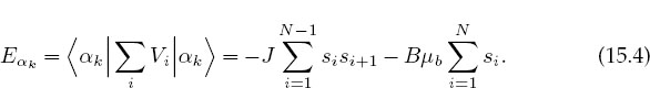
The energy of this system in state α_k is the expectation value of the sum of the potential V over the spins of the particles:

An apparent paradox in the Ising model occurs when we turn off the external magnetic field and thereby eliminate a preferred direction in space. This means that the average magnetization should vanish even though the lowest energy state would have all spins aligned. The answer to this paradox is that the system with B = 0 is unstable. Even if all the spins are aligned, there is nothing to stop their spontaneous reversal. Indeed, natural magnetic materials have multiple finite domains with all the spins aligned, but with the different domains pointing in different directions. The instabilities in which domains change direction are called Bloch-wall transitions. For simplicity we assume B = 0, which means that the spins interact just with each other. However, be cognizant of the fact that this means there is no preferred direction in space, and so you may have to be careful how you calculate observables. For example, you may need to take an absolute value of the total spin when calculating the magnetization, that is, to calculate <|Σi si|> rather than (Σi si).

The equilibrium alignment of the spins depends critically on the sign of the exchange energy J. If J > 0, the lowest energy state will tend to have neighboring spins aligned. If the temperature is low enough, the ground state will be aferro-magnet with all the spins aligned. If J < 0, the lowest energy state will tend to have neighbors with opposite spins. If the temperature is low enough, the ground state will be a antiferromagnet with alternating spins.

The simple 1-D Ising model has its limitations. Although the model is accurate in describing a system in thermal equilibrium, it is not accurate in describing the approach to thermal equilibrium (nonequilibrium thermodynamics is a difficult subject for which the theory is not complete). Second, as part of our algorithm we postulate that only one spin is flipped at a time, while real magnetic materials tend to flip many spins at a time. Other limitations are straightforward to improve, for example, the addition of longer-range interactions, the motion of the centers, higher-multiplicity spin states, and two and three dimensions.

A fascinating aspect of magnetic materials is the existence of a critical temperature, the Curie temperature, above which the gross magnetization essentially vanishes. Below the Curie temperature the quantum state of the material has long-range order extending over macroscopic dimensions; above the Curie temperature there is only short-range order extending over atomic dimensions. Even though the 1-D Ising model predicts realistic temperature dependences for the thermodynamic quantities, the model is too simple to support a phase transition. However, the 2-D and 3-D Ising models do support the Curie temperature phase transition.

15.3 Statistical Mechanics (Theory)

Statistical mechanics starts with the elementary interactions among a system’s particles and constructs the macroscopic thermodynamic properties such as specific heats. The essential assumption is that all configurations of the system consistent with the constraints are possible. In some simulations, such as the molecular dynamics ones in Chapter 16, “Simulating Matter with Molecular Dynamics,” the problem is set up such that the energy of the system is fixed. The states of this type of system are described by what is called a microcanonical ensemble. In contrast, for the thermodynamic simulations we study in this chapter, the temperature, volume, and number of particles remain fixed, and so we have what is called a canonical ensemble.

When we say that an object is at temperature T, we mean that the object’s atoms are in thermodynamic equilibrium at temperature T such that each atom has an average energy proportional to T. Although this may be an equilibrium state, it is a dynamic one in which the object’s energy fluctuates as it exchanges energy with its environment (it is thermo dynamics after all). Indeed, one of the most illuminating aspects of the simulation we shall develop is its visualization of the continual and random interchange of energy that occurs at equilibrium.

The energy E_αj of state α_j in a canonical ensemble is not constant but is distributed with probabilities P(α_j) given by the Boltzmann distribution:

Here k is Boltzmann’s constant, T is the temperature, and Z(T) is the partition function, a weighted sum over states. Note that the sums in (15.5) are over the individual states or configurations of the system. Another formulation, such as the Wang–Landau algorithm in Unit II, sums over the energies of the statesof the system and includes a density-of-states factor g(E_i) to account for degenerate states with the same energy. While the present sum over states is a simpler way to express the problem (one less function), we shall see that the sum over energies is more efficient numerically. In fact, in this unit we even ignore the partition function Z(T) because it cancels out when dealing with the ratio of probabilities.

15.3.1 Analytic Solutions

For very large numbers of particles, the thermodynamic properties of the 1-D Ising model can be solved analytically and determine [P&B 94]

The analytic results for the specific heat per particle and the magnetization are

The 2-D Ising model has an analytic solution, butitwas not easytoderive [Yang 52, Huang 87]. Whereas the internal energy and heat capacity are expressed in terms of elliptic integrals, the spontaneous magnetization per particle has the rather simple form

where the temperature is measured in units of the Curie temperature Tc.

15.4 Metropolis Algorithm

In trying to devise an algorithm that simulates thermal equilibrium, it is important to understand that the Boltzmann distribution (15.5) does not require a system to remain in the state of lowest energy but says that it is less likely for the system to be found in a higher-energy state than in a lower-energy one. Of course, as T → 0, only the lowest energy state will be populated. For finite temperatures we expect the energy to fluctuate by approximately k_BT about the equilibrium value.

In their simulation of neutron transmission through matter, Metropolis, Rosenbluth, Teller, and Teller [Metp 53] invented an algorithm to improve the Monte Carlo calculation of averages. This Metropolis algorithm is now a cornerstone of computational physics. The sequence of configurations it produces (a Markov chain) accurately simulates the fluctuations that occur during thermal equilibrium. The algorithm randomly changes the individual spins such that, on the average, the probability of a configuration occurring follows a Boltzmann distribution. (We do not find the proof of this trivial or particularly illuminating.)

The Metropolis algorithm is a combination of the variance reduction technique discussed in §6.7.1 and the von Neumann rejection technique discussed in §6.7.3. There we showed how to make Monte Carlo integration more efficient by sampling random points predominantly where the integrand is large and how to generate random points with an arbitrary probability distribution. Now we would like to havespinsfliprandomly, haveasystem thatcanreach anyenergyinafinite number of steps (ergodic sampling), have a distribution of energies described by a Boltz-mann distribution, yet have systems that equilibrate quickly enough to compute in reasonable times.

The Metropolis algorithm is implemented via a number of steps. We start with a fixed temperature and an initial spin configuration and apply the algorithm until a thermal equilibrium is reached (equilibration). Continued application of the algorithm generates the statistical fluctuations about equilibrium from which we deduce the thermodynamic quantities such as the magnetization M(T). Then the temperature is changed, and the whole process is repeated in order to deduce the T dependence of the thermodynamic quantities. The accuracy of the deduced temperature dependences provides convincing evidence for the validity of the algorithm. Because the possible 2^N configurations of N particles can be a very large number, the amount of computer time needed can be very long. Typically, a small number of iterations 10N is adequate for equilibration.

The explicit steps of the Metropolis algorithm are as follows.

The heartofthis algorithmisits generationofarandom spin configuration α_j (15.2) with probability

The technique is a variation of von Neumann rejection (stone throwing in §6.5) in which a random trial configuration is either accepted or rejected depending upon the value of the Boltzmann factor. Explicitly, the ratio of probabilities for a trial configuration of energy E_t to that of an initial configuration of energy E_i is

Figure 15.2 A 1-D lattice of 100 spins aligned along the ordinate. Up spins are indicated by circles,and down spins by blank spaces. The iteration number (“time”) dependence of the spins is shown along the abscissa. Even though the system starts with all up spins (a“cold” start), the system is seen to form domains as it equilibrates.

If the trial configuration has a lower energy (ΔE ≤ 0), the relative probability will be greater than 1 and we will accept the trial configuration as the new initial configuration without further ado. However, if the trial configuration has a higher energy (ΔE > 0), we will not reject it out of hand but instead accept it with relative probability R = exp(— Δ E/k_BT) < 1. To accept a configuration with a probability we pick a uniform random number between 0 and 1, and if the probability is greater than this number, we accept the trial configuration; if the probability is smaller than the chosen random number, we reject it. (You can remember which way this goes by letting Eα_tr → ∞, in which case P → 0 and nothing is accepted.) When the trial configuration is rejected, the next configuration is identical to the preceding one.

How do you start? One possibility is to start with random values of the spins (a “hot” start). Another possibility (Figure 15.2) is a “cold” start in which you start with all spins parallel (J > 0) or antiparallel (J < 0). In general, one tries to remove the importance of the starting configuration by letting the calculation run a while (10N rearrangements) before calculating the equilibrium thermodynamic quantities. You should get similar results for hot, cold, or arbitrary starts, and by taking their average you remove some of the statistical fluctuations.

15.4.1 Metropolis Algorithm Implementation

15.4.2 Equilibration, Thermodynamic Properties (Assessment)

Listing 15.1 Ising.java implements the Metropolis algorithm for a 1-D Ising chain.

Thermodynamic Properties: For a given spin configuration α_j, the energy and magnetization are given by

The internal energy U(T) is just the average value of the energy,

where the average is taken over a system in equilibrium. At high temperatures we expect a random assortment of spins and so a vanishing magnetization. At low temperatures when all the spins are aligned, we expect M to approach N/2. Although the specific heat can be computed from the elementary definition

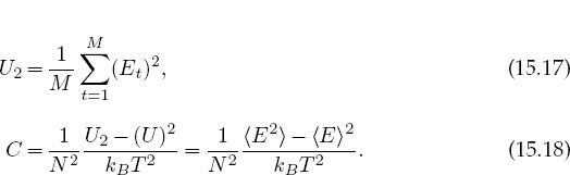
the numerical differentiation may be inaccurate since U has statistical fluctuations. A better way to calculate the specific heat is to first calculate the fluctuations in energy occurring during M trials and then determine the specific heat from the fluctuations:

Figure 15.3 Simulation results for the energy, specific heat, and magnetization of a 1-D lattice of 100 spins as a function of temperature.

15.4.3 Beyond Nearest Neighbors and 1-D (Exploration)

Exercise: Three fixed spin-½ particles interact with each other at temperature T = 1/k_b such that the energy of the system is

The system starts in the configuration ↑↓↑. Do a simulation by hand that uses the Metropolis algorithm and the series of random numbers 0.5, 0.1, 0.9, 0.3 to determine the results of just two thermal fluctuations of these three spins.

15.5 Unit II. Magnets via Wang–Landau Sampling

In Unit I we used a Boltzmann distribution to simulate the thermal properties of an Ising model. There we described the probabilities for explicit spin states α with energy E_α for a system at temperature T and summed over various configurations. An equivalent formulation describes the probability that the system will have the explicit energy E at temperature T:

Figure 15.4 The energy, specific heat,and magnetization as a function of temperature for a 2-D lattice with 40,000 spins. The values of C and E have been scaled to fit on the same plot as M. (Courtesy of J. Wetzel.)

Here k_B is Boltzmann’s constant, T is the temperature, g(E_i) is the number of states of energy E_i (i = 1,…, M), Z(T) is the partition function, and the sum is still over all M states of the system but now with states of the same energy entering just once owing to g(E_i) accounting for their degeneracy. Because we again apply the theory to the Ising model with its discrete spin states, the energy also assumes only discrete values. If the physical system had an energy that varied continuously, then the number of states in the interval E → E +dE would be given by g(E)dE and g(E) would be called the density of states. As a matter of convenience, we call g(E_i) the density of states even when dealing with discrete systems, although the term “degeneracy factor” may be more precise.

Even as the Metropolis algorithm has been providing excellent service for more than 50 years, recent literature shows increasing use of Wang–Landau sampling (WLS) [WL 04, Clark]. Because WLS determines the density of states and the associated partition function, it is not a direct substitute for the Metropolis algorithm and its simulation of thermal fluctuations. However, we will see that WLS provides an equivalent simulation for the Ising model.² Nevertheless, there are cases where the Metropolis algorithm can be used but WLS cannot, computation of the ground-state function of the harmonic oscillator (Unit III) being an example.

The advantages of WLS is that it requires much shorter simulation times than the Metropolis algorithm and provides a direct determination of g(Ei). For these reasons it has shown itself to be particularly useful for first-order phase transitions where systems spend long times trapped in metastable states, as well as in areas as diverse as spin systems, fluids, liquid crystals, polymers, and proteins. The time required for a simulation becomes crucial when large systems are modeled. Even a spin lattice as small as 8 × 8 has 2⁶⁴ 1.84 × 10¹⁹ configurations, and it would be too expensive to visit them all.

In Unit I we ignored the partition function when employing the Metropolis algorithm. Now we focus on the partition function Z(T) and the density-of-states function g(E). Because g(E) is a function of energy but not temperature, once it has been deduced, Z(T) and all thermodynamic quantities can be calculated from it without having to repeat the simulation for each temperature. For example, the internal energy and the entropy are calculated directly as

The density of states g(E_i) will be determined by taking the equivalent of a random walk in energy space. We flip a randomly chosen spin, record the energy of the new configuration, and then keep walking by flipping more spins to change the energy. The table H(E_i) of the number of times each energy E_i is attained is called the energy histogram (an example of why it is called a histogram is given in Figure 15.5 on the right). If the walk were continued for a very long time, the histogram H(E_i) would converge to the density of states g(E_i). Yet with 10¹⁹–10³⁰ steps required even for small systems, this direct approach is unrealistically inefficient because the walk would rarely ever get away from the most probable energies.

Clever idea number 1 behind the Wang–Landau algorithm is to explore more of the energy space by increasing the likelihood of walking into less probable configurations. This is done by increasing the acceptance of less likely configurations while simultaneously decreasing the acceptance of more likely ones. In other words, we want to accept more states for which the density g(E_i) is small and reject more states for which g(E_i) is large (fret not these words, the equations are simple). To accomplish this trick, we accept a new energy E_i with a probability inversely proportional to the (initially unknown) density of states,

Figure 15.5 Left: Logarithm of the density of states log g(E) ∝ S versus the energy per particle for a 2-D Ising model on an 8×8 lattice. Right: The histogram H(E) showing the number of states visited as a function of the energy per particle. The aim of WLS is to make this function flat.

and then build up a histogram of visited states via a random walk.

The problem with clever idea number 1 is that g(E_i) is unknown. WLS’s clever idea 2 is to determine the unknown g(E_i) simultaneously with the construction of the random walk. This is accomplished by improving the value of g(E_i) via the multiplication g(E_i) → f g(E_i), where f > 1 is an empirical factor. When this works, the resulting histogram H(E_i) becomes “flatter” because making the small g(E_i) values larger makes it more likely to reach states with small g(E_i) values. As the histogram gets flatter, we keep decreasing the multiplicative factor f until it is satisfactory close to 1. At that point we have a flat histogram and a determination of g(E_i).

At this point you may be asking yourself, “Why does a flat histogram mean that we have determined g(E_i)?” Flat means that all energies are visited equally, in contrast to the peaked histogram that would be obtained normally without the 1/g(E_i) weighting factor. Thus, if by including this weighting factor we produce a flat histogram, then we have perfectly counteracted the actual peaking in g(E_i), which means that we have arrived at the correct g(E_i).

15.6 Wang–Landau Sampling

The steps in WLS are similar to those in the Metropolis algorithm, but now with use of the density-of-states function g(E_i) rather than a Boltzmann factor:

Figure 15.6 The numbering scheme used for our 8×8 2-D lattice of spins.

15.6.1 WLS Ising Model Implementation

We assume an Ising model with spin–spin interactions between nearest neighbors located in an L×L lattice (Figure 15.6). To keep the notation simple, we set J = 1 so that

where ↔ indicates nearest neighbors. Rather than recalculate the energy each time a spin is flipped, only the difference in energy is computed. For example, for eight spins in a 1-D array,

where the 0–7 interaction arises because we assume periodic boundary conditions. If spin 5 is flipped, the new energy is

and the difference in energy is

This is cheaper to compute than calculating and then subtracting two energies.

When we advance to two dimensions with the 8 × 8 lattice in Figure 15.6, the change in energy when spin σi,j flips is

which can assume the values -8,-4,0,4, and 8. There are two states of minimum energy -2N for a 2-D system with N spins, and they correspond to all spins pointing in the same direction (either up or down). The maximum energy is +2N, and it corresponds to alternating spin directions on neighboring sites. Each spin flip on the lattice changes the energy by four units between these limits, and so the values of the energies are

These energies can be stored in a uniform 1-D array via the simple mapping

Listing 15.2 displays our implementation of Wang–Landau sampling to calculate the density of states and internal energy U(T) (15.20). We used it to obtain the entropy S(T) and the energy histogram H(E_i) illustrated in Figure 15.5. Other thermodynamic functions can be obtained by replacing the E in (15.20) with the appropriate variable. The results look like those in Figure 15.4.Aproblem that may be encountered when calculating these variables is that the sums in (15.20) can become large enough to cause overflows, even though the ratio would not. You work around that by factoring out a common large factor; for example,

where λ is the largest value of ln g(E_i)-Ei/k_BT at each temperature. The factor eλ does not actually need to be included in the calculation of the variable because it is present in both the numerator and denominator and so cancels out.

Listing 15.2 WangLandau.java simulates the 2-D Ising model using Wang–Landau sampling to compute the density of states and from that the internal energy.

15.6.2 WLS Ising Model Assessment

Repeat the assessment conducted in §15.4.2 for the thermodynamic properties of the Ising model but use WLS in place of the Metropolis algorithm.

15.7 Unit III. Feynman Path Integrals

Problem: As is well known, a classical particle attached to a linear spring undergoes simple harmonic motion with a position in space as a function of time given by x(t) = A sin(ω_ot + φ). Your problem is to take this classical space-time trajectory x(t) and use it to generate the quantum wave function ψ(x, t) for a particle bound in a harmonic oscillator potential.

15.8 Feynman’s Space-Time Propagation (Theory)

Feynman was looking for a formulation of quantum mechanics that gave a more direct connection to classical mechanics than does Schrödinger theory and that made the statistical nature of quantum mechanics evident from the start. He followed a suggestion by Dirac that Hamilton’s principle of least action, which can be used to derive classical mechanics, may be the → 0 limit of a quantum least-action principle. Seeing that Hamilton’s principle deals with the paths of particles through space-time, Feynman posultated that the quantum wave function describing the propagation of a free particle from the space-time point a = (x_a,t_a) to the point b = (x_b, t_b) can expressed as [F&H 65]

where G is the Green’s function or propagator

Equation (15.39) is a form of Huygens’s wavelet principle in which each point on the wavefront ψ(x_a,t_a) emits a spherical wavelet G(b;a) that propagates forward in space and time. It states that a new wavefront ψ(x_b,t_b) is created by summation over and interference with all the other wavelets.

Feynman imagined that another way of interpreting (15.39) is as a form of Hamilton’s principle in which the probability amplitude (wave function ψ) for a particle to be at B is equal to the sum over all paths through space-time originating at time A and ending at B (Figure 15.7). This view incorporates the statistical nature of quantum mechanics by having different probabilities for travel along the different paths. All paths are possible, but some are more likely than others. (When you realize that Schrödinger theory solves for wave functions and considers paths a classical concept, you can appreciate how different it is from Feynman’s view.) The values for the probabilities of the paths derive from Hamilton’s classical principle of least action:

Figure 15.7 A collection of paths connecting the initial space-time point A to the final point B. The solid line is the trajectory followed by a classical particle, while the dashed lines are additional paths sampled by a quantum particle. A classical particle somehow “knows” ahead of time that travel along the classical trajectory minimizes the action S.

The most general motion of a physical particle moving along the classical trajectory x(t) from time ta to tb is along a path such that the action S[x ¯(t)] is an extremum:

with the paths constrained to pass through the endpoints:

This formulation of classical mechanics, which is based on the calculus of variations, is equivalent to Newton’s differential equations if the action S is taken as the line integral of the Lagrangian along the path:

Here T is the kinetic energy, V is the potential energy, = dx/dt, and square brackets indicate a functional³ of the function x(t) and (t).

Feynman observed that the classical action for a free particle (V = 0),

is related to the free-particle propagator (15.40) by

This is the much sought connection between quantum mechanics and Hamilton’s principle. Feynman then postulated a reformulation of quantum mechanics that incorporated its statistical aspects by expressing G(b, a) as the weighted sum over all paths connecting a to b,

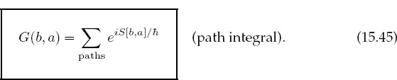
Here the classical action S (15.42) is evaluated along different paths (Figure 15.7), and the exponential of the action is summed over paths. The sum (15.45) is called a path integral because it sums over actions S[b, a], each of which is an integral (on the computer an integral and a sum are the same anyway). The essential connection between classical and quantum mechanics is the realization that in units of 10-³⁴ Js, the action is a very large number, S/ ≥ 10²⁰, and so even though all paths enter into the sum (15.45), the main contributions come from those paths adjacent to the classical trajectory x. In fact, because S is an extremum for the classical trajectory, it is a constant to first order in the variation of paths, and so nearby paths have phases that vary smoothly and relatively slowly. In contrast, paths far from the classical trajectory are weighted by a rapidly oscillating exp(iS/), and when many are included, they tend to cancel each other out. In the classical limit, → 0, only the single classical trajectory contributes and (15.45) becomes Hamilton’s principle of least action! In Figure 15.8 we show an example of a trajectory used in path-integral calculations.

Figure 15.8 Left: The probability distribution for the harmonic oscillator ground state as determined with a path-integral calculation (the classical result has maxima at the two turning points). Right: A space-time trajectory used as a quantum path.

15.8.1 Bound-State Wave Function (Theory)

Although you may be thinking that you have already seen enough expressions for the Green’s function, there is yet another one we need for our computation. Let us assume that the Hamiltonian H supports a spectrum of eigenfunctions,

each labeled by the index n. Because H is Hermitian, the solutions form a complete orthonormal set in which we may expand a general solution:

where the value for the expansion coefficients c_n follows from the orthonormality of the ψ_n’s. If we substitute this c_n back into the wave function expansion (15.46), we obtain the identity

Comparison with (15.39) yields the eigenfunction expansion for G:

We relate this to the bound-state wave function (recall that our problem is to calculate that) by (1) requiring all paths to start and end at the space position x₀ = x, (2) by taking t₀ = 0, and (3) by making an analytic continuation of (15.48) to negative imaginary time (permissable for analytic functions):

The limit here corresponds to long imaginary times τ, after which the parts of ψ with higher energies decay more quickly, leaving only the ground state ψ₀.

Equation (15.49) provides a closed-form solution for the ground-statewave function directly in terms of the propagator G. Although we will soon describe how to compute this equation, look now at Figure 15.8 showing some resultsof a computation. Although we start with a probability distribution that peaks near the classical turning points at the edges of the well, after a large number of iterations we end up with a distribution that resembles the expected Gaussian. On the right we see a trajectory that has been generated via statistical variations about the classical trajectory x(t) = A sin(ω₀t + ø).

15.8.2 Lattice Path Integration (Algorithm)

Because both time and space are integrated over when evaluating a path integral, we set up a lattice of discrete points in space-time and visualize a particle’s trajectory as a series of straight lines connecting one time to the next (Figure 15.9). We divide the time between points A and B into N equal steps of size ε and label them with the index j:

Although it is more precise to use the actual positions x(t_j) of the trajectory at the times t_j to determine the x_js (as in Figure 15.9), in practice we discretize space uniformly and have the links end at the nearest regular points. Once we have a lattice, it is easy to evaluate derivatives or integrals on a link⁴:

where we have assumed that the Lagrangian is constant over each link.

Figure 15.9 Left: A path through the space-time lattice that starts and ends at x_a = x_b. The action is an integral over this path, while the path integral is a sum of integrals over all paths. The dotted path BD is a transposed replica of path AC. Right: The dashed path joins the initial and final times in two equal time steps; the solid curve uses N steps each of size ε. The position of the curve at time t_j defines the position x_j.

Lattice path integration is based on the composition theorem for propagators:

where we have added the actions since line integrals combine as S[b, j]+ S[j, a] = S[b, a]. For the N-linked path in Figure 15.9, equation (15.53) becomes

where S_j is the value of the action for link j. At this point the integral over the single path shown in Figure 15.9 has become an N-term sum that becomes an infinite sum as the time step ε approaches zero.

To summarize, Feynman’s path-integral postulate (15.45) means that we sum over all paths connecting A to B to obtain Green’s function G(b, a). This means that we must sum not only over the links in one path but also over all the different paths in order to produce the variation in paths required by Hamilton’s principle. The sum is constrained such that paths must pass through A and B and cannot double back on themselves (causality requires that particles move only forward in time). This is the essence of path integration. Because we are integrating over functions as well as along paths, the technique is also known as functional integration.

The propagator (15.45) is the sum over all paths connecting A to B, with each path weighted by the exponential of the action along that path, explicitly:

where L(x_j, _j) is the average value of the Lagrangian on link j at time t = jε. The computation is made simpler by assuming that the potential V (x) is independent of velocity and does not depend on other x values (local potential). Next we observe that G is evaluated with a negative imaginary time in the expression (15.49) for the ground-state wave function. Accordingly, we evaluate the Lagrangian with t = —iτ:

We see that the reversal of the sign of the kinetic energy in L means that L now equals the negative of the Hamiltonian evaluated at a real positive time t = τ:

In this way we rewrite the t-path integral of L as a τ-path integral of H and so express the action and Green’s function in terms of the Hamiltonian:

where the line integral of H is over an entire trajectory. Next we express the path integral in terms of the average energy of the particle on each link, Ej = Tj +Vj, and then sum over links⁵ to obtain the summed energy ε:

In (15.65) we have approximated each path link as a straight line, used Euler’s derivative rule to obtain the velocity, and evaluated the potential at the midpoint of each link. We now substitute this G into our solution (15.49) for the ground-state wave function in which the initial and final points in space are the same:

The similarity of these expressions to thermodynamics, even with a partition function Z, is no accident; by making the time parameter of quantum mechanics imaginary, we have converted the time-dependent Schrödinger equation to the heat diffusion equation:

It is not surprising then that the sum over paths in Green’s function has each path weighted by the Boltzmann factor usually associated with thermodynamics. We make the connection complete by identifying the temperature with the inverse time step:

Consequently, the ε → 0 limit, which makes time continuous, is a “high-temperature” limit. The τ → ∞ limit, which is required to project the ground-state wave function, means that we must integrate over a path that is long in imaginary time, that is, long compared to a typical time / ΔE. Just as our simulation of the Ising model in Unit I required us to wait a long time while the system equilibrated, so the present simulation requires us to wait a long time so that all but the ground-state wave function has decayed. Alas, this is the solution to our problem of finding the ground-state wave function.

To summarize, we have expressed the Green’s function as a path integral that requires integration of the Hamiltonian along paths and a summation over all the paths (15.66). We evaluate this path integral as the sum over all the trajectories in a space-time lattice. Each trial path occurs with a probability based on its action, and we use the Metropolis algorithm to include statistical fluctuation in the links, as if they are in thermal equilibrium. This is similar to our work with the Ising model in Unit I, however now, rather than reject or accept a flip in spin based on the change in energy, we reject or accept a change in a link based on the change in energy. The more iterations we let the algorithm run for, the more time the deduced wave function has to equilibrate to the ground state.

In general, Monte Carlo Green’s function techniques work best if we start with a good guess at the correct answer and have the algorithm calculate variations on our guess. For the present problem this means that if we start with a path in space-time close to the classical trajectory, the algorithm may be expected to do a good job at simulating the quantum fluctuations about the classical trajectory. However, it does not appear to be good at finding the classical trajectory from arbitrary locations in space-time. We suspect that the latter arises from δS/ being so large that the weighting factor exp(δS/) fluctuates wildly (essentially averaging out to zero) and so loses its sensitivity.

15.8.2.1 A TIME-SAVING TRICK

As we have formulated the computation, we pick a value of x and perform an expensive computation of line integrals over all space and time to obtain |ψ₀(x)| at one x. To obtain the wave function at another x, the entire simulation must be repeated from scratch. Rather than go through all that trouble again and again, we will compute the entire x dependence of the wave function in one fell swoop. The trick is to insert a delta function into the probability integral (15.66), thereby fixing the initial position to be x₀, and then to integrate over all values for x₀:

This equation expresses the wave function as an average of a delta function over all paths, a procedure that might appear totally inappropriate for numerical computation because there is tremendous error in representing a singular function on a finite-word-length computer. Yet when we simulate the sum over all paths with (15.71), there will always be some x value for which the integral is nonzero, and we need to accumulate only the solution for various (discrete) x values to determine |ψο(x) |² for allx.

To understand how this works in practice, consider path AB in Figure 15.9 for which we have just calculated the summed energy. We form a new path by having one point on the chain jump to point C (which changes two links). If we replicate section AC and use it as the extension AD to form the top path, we see that the path CBD has the same summed energy (action) as path ACB and in this way can be used to determine |ψ₀(x’)|^2. That being the case, once the system is equilibrated, we determine new values of the wave function at new locations x’j by flipping links to new values and calculating new actions. The more frequently some x_j is accepted, the greater the wave function at that point.

15.8.3 Lattice Implementation

The program QMC.java in Listing 15.3 evaluates the integral (15.45) by finding the average of the integrand δ(x₀ – x) with paths distributed according to the weighting function exp[-εε(x₀, x₁,…, x_N)]. The physics enters via (15.73), the calculation of the summed energy ε(x₀,x₁,…, x_N). We evaluate the action integral for the harmonic oscillator potential

and for a particle of mass m = 1. Using a convenient set of natural units, we measure lengths in Correspondingly, the oscillator has a period Τ = 2π. Figure 15.8 shows results from an application of the Metropolis algorithm. In this computation we started with an initial path close to the classical trajectory and then examined _½ million variations about this path. All paths are constrained to begin and end at x = 1 (which turns out to be somewhat less than the maximum amplitude of the classical oscillation).

When the time difference t_b – t_a equals a short time like 2T, the system has not had enough time to equilibrate to its ground state and the wave function looks like the probability distribution of an excited state (nearly classical with the probability highest for the particle to be near its turning points where its velocity vanishes). However, when t_b – t_a equals the longer time 20T, the system has had enough time to decay to its ground state and the wave function looks like the expected Gaussian distribution. In either case (Figure 15.8 right), the trajectory through space-time fluctuates about the classical trajectory. This fluctuation is a consequence of the Metropolis algorithm occasionally going uphill in its search; if you modify the program so that searches go only downhill, the space-time trajectory will be a very smooth trigonometric function (the classical trajectory), but the wave function, which is a measure of the fluctuations about the classical trajectory, will vanish! The explicit steps of the calculation are

Listing 15.3 QMC.java solves for the ground-state probability distribution via a Feynman path integration using the Metropolis algorithm to simulate variations about the classical trajectory.

15.8.4 Assessment and Exploration

15.9 Exploration: Quantum Bouncer’s Paths

Another problem for which the classical trajectory is well known is that of a quantum bouncer. Here we have a particle dropped in a uniform gravitational field, hitting a hard floor, and then bouncing. When treated quantum mechanically, quantized levels for the particle result [Gibbs 75, Good 92, Whine 92, Bana 99, Vall 00]. In 2002 an experiment to discern this gravitational effect at the quantum level was performed by Nesvizhevsky et al. [Nes 02] and described in [Schw 02]. It consisted of dropping ultracold neutrons from a height of 14 µm unto a neutron mirror and watching them bounce. It found a neutron ground state at 1.4 peV.

We start by determining the analytic solution to this problem for stationary states and then generalize it to include time dependence.⁶ The time-independent Schrödinger equation for a particle in a uniform gravitation potential is

The boundary condition (15.75)is a consequence of the hard floor at x = 0. A change of variables converts (15.74) to a dimensionless form,

This equation has an analytic solution in terms of Airy functions Ai(z) [L 96]:

Figure 15.10 The Airy function squared (continuous line) and the Quantum Monte Carlo solution |ψ₀(q)|² (dashed line) after a million trajectories.

where N_n is a normalization constant and z_E is the scaled value of the energy. The boundary condition ψ(0) = 0 implies that

which means that the allowed energies of the system are discrete and correspond to the zeros z_n of the Airy functions [Pres 00] at negative argument. To simplify the calculation, we take = 1, g = 2, and m = ½, which leads to z = x and z_E = E.

The time-dependent solution for the quantum bouncer is constructed by forming the infinite sum over all the discrete eigenstates, each with a time dependence appropriate to its energy:

where the Cn’s are constants.

Figure 15.10 shows the results of solving for the quantum bouncer’s ground-state probability |ψ ₀(z)|² using Feynman’s path integration. The time increment dt and the total time t were selected by trial and error in such away as to make |ψ(0)|² 0 (the boundary condition). To account for the fact that the potential is infinite for negative x values, we selected trajectories that have positive x values over all their links. This incorporates the fact that the particle can never penetrate the floor. Our program is given in Listing 15.4, and it yields the results in Figure 15.10 after using 10⁶ trajectories and a time step ε = dτ = 0.05. Both results were normalized via a trapezoid integration. As can be seen, the agreement between the analytic result and the path integration is satisfactory.

Listing 15.4 QMCbouncer.java uses Feynman path integration to compute the path of a quantum particle in a gravitational field.

1 Large-scale, practical computations make a full sweep in which every spin is updated once and then use this as the new trial configuration. This is found to be more efficient and useful in removing some autocorrelations. (We thank G. Schneider for this observation.)

2 We thank Oscar A. Restrepo of the Universidad de Antioquia for letting us use some of his material here.

3 Afunctional is a number whose value depends on the complete behavior of some function and not just on its behavior at one point. For example, the derivative f’(x) depends on the value of f at x, yet the integral depends on the entire function and is therefore a functional of f.

4 Even though Euler’s rule has a large error, it is often use in lattice calculations because of its simplicity. However, if the Lagrangian contains second derivatives, you should use the more precise central-difference method to avoid singularities.

5 In some cases, such as for an infinite square well, this can cause problems if the trial link causes the energy to be infinite. In that case, one can modify the algorithm to use the potential at the beginning of a link

6 Oscar A. Restrepo assisted in the preparation of this section.