11 Mapping and Multimode Radars

11.1 INTRODUCTION

Airborne ground-mapping radars were originally developed in World War II as a means of bombing through clouds and weather—and at night, when the bombing-aircraft operator could not see his target visually. These radars performed two navigation functions. First, they permitted the aircraft to find its way over enemy terrain, without ground navigation aids or sight of the ground, to the threshold of the bombing run. Second, the radar then provided precise navigation during the bombing run by use of cursors set on the target point in a display. Later, a “beacon” mode was added to enable the radar to make fixes on beacon transponders placed at known ground positions in friendly territory and coded to establish their identity. This permitted much easier and more precise navigation by radar during the early phases of the inbound leg to the target and, more important, on return. It was also found that the radar could be used to see intense storms and navigate around them during times of darkness or flight through clouds.

These early radars illustrate the major themes that have concerned navigation radar designers ever since, namely, general navigation; precision navigation for landing, weapon delivery, air drop of personnel and material; and beacon navigation.

Radar-navigation economics also remain much the same. First, a ground-mapping radar is heavier, more expensive, and complex compared to navigation equipment aided by either ground-based systems, such as VOR, Loran, and Omega, or spaced-based equipment, such as GPS. Second, it is uneconomical in comparison with specialized self-contained navigation equipment, such as dedicated Doppler-navigation radars and inertial sensors. However, in regions like the Arctic and Antarctic, where there are few ground aids, wilderness areas, and hostile terrain in combat zones, radars may be the only source of accurate navigation data. Radar navigation became economically attractive with the advent of high-speed, programmable signal and data processors. Then a single radar could perform a multitude of functions solely through additions to software. For example, weather avoidance or weather penetration modes, which are direct descendants of the storm-detection functions of the World War II radars, can be performed by the multimode radar. Other navigation modes implemented through software in multimode radars are terrain avoidance (TA) and terrain following (TF) for low-level flight by military aircraft operation in hostile territory, determination of altitude (AGR), and determination of speed and drift (PVU) for improved dead reckoning.

A less obvious economic factor that is at work in favor of multimode radars is the steady increase in the size and expense of transport aircraft. The great cost of these aircraft and the large number of people they carry makes it imperative that very great safety of operation be obtained. This may make it attractive to add navigation landing-aid modes to the pure weather radars used by commercial airlines.

Another factor at work is the rapid improvement in the reliability and maintainability of current radars. The techniques for producing high reliability by proper design and manufacturing methods have become highly developed in recent years. Radar mean-time-between-failure (MTBF) has risen from tens to hundreds of hours over a very short time span. In addition, analog and digital circuit miniaturization has allowed fault detection and isolation technology to be incorporated down to the most critical complex component. Circuits cards perform self-tests as a background task and report the results to the system's built-in-test (BIT) function when requested. Thus, when the radar does fail, isolation to and identification of the failed complex component is instantaneous. The repair philosophy is to replace the failed module with a spare module. A remote repair facility utilizes the stored BIT codes to select a failed complex component for replacement. Thus, on-site repair work is reduced to a task requiring little skill, and the necessity of keeping highly skilled radar technicians at every airport along each route—an economic impossibility—is eliminated.

11.2 RADAR PILOTAGE

The most common method of position fixing by radar navigation is completely analogous to aircraft pilotage by visual reference. The pilot corrects his heading by observing the terrain around him as a maplike image on the radar display. However, the scale of usable reference points in radar is different. Visually, roads, lakes, parks, railroads, and rivers are most useful for reference when they are within 10 mi of the aircraft. Since radars have narrow antenna beamwidths, typically, 3 to 6 deg, they do not have the eye's field of view and cannot find as many reference points instantaneously. Thus, a sequence of radar modes is employed. Figure 11.1 illustrates the progressive magnification of terrain. First, the radar utilizes the real beam ground map (RBGM) modes to scan a large angular and range sector from a great distance with coarse resolution to find suitable large reference points for initial acquisition. Second, the radar employs the Doppler beam sharpening (DBS) mode to decrease its field of view about the selected ground point, magnify the radar image with moderate resolution, and refine the acquisition. Third, a fine resolution image with narrow field of view is generated using the synthetic array radar (SAR) mode and utilized for final designation and position update. The initial acquisition scan has resolution such that towns, cities, lakes, and rivers can be recognized at distances as great as 160 nmi from the aircraft. Subsequent, finer resolution radar images have resolution such that individual streets within a city or specific terrain features, such as road intersections, can be recognized at ranges as large as 50 nmi. Radar resolution required to identify terrain and cultural features is summarized in Table 11.1.

Figure 11.1 RBGM, DBS, SAR coverage shown on RBGM display.

In the use of references points, radar has an advantage because in visual pilotage the distance to an object and its angular position with respect to the aircraft must be estimated. This can be done with adequate accuracy at low altitudes: however, at high altitudes, distances are very difficult to judge with visual pilotage, even in clear weather. With radar pilotage, accurate range and angle measurements can be made by superimposing range and azimuth markers on the radar image feature selected for the update point and instructing the radar to compute the aircraft position vector relative to the update point.

TABLE 11.1 Radar image resolution requirements

The radar display format used for initial acquisition is the plan-position-indicator (PPI) format. A large azimuth angular region, typically 120 deg, about the aircraft velocity vector is scanned, and the radar collects a few pulses of noncoherent radar return over a large range interval, 20 to 160 nmi dependent upon the range scale chosen, at each antenna beam position. RBGM images are formed in the radar signal processor and stored digitally in its memory as an amplitude, range bin, azimuth angle matrix. To display these data to the pilot in a geometrically correct format, the range bin amplitudes for each antenna beam position, or range trace, are read sequentially from the processor memory and “painted” on the display along a radial sweep with azimuth angle corresponding to the antenna's position relative to a display reference angle, typically North up or aircraft velocity vector up, at the time of data collection. The range trace starts at a range slightly larger than the range corresponding to the width of the transmitted pulse, or “main bang,” and proceeds to a range corresponding to the maximum number of range bins that are processed.

Typically, radars collect 256 to 512 range samples of data from each radar pulse and vary the range bin width to provide range scales from 20 to 160 nmi. Once the first range trace of data is displayed, the radar retrieves the second range trace of data and “paints” it on the display along a radial corresponding to the azimuth angle of the antenna when that data were collected. This retrieval and display “painting” process continues until all data collected during the scan are displayed. Then, the next scan of data is retrieved and displayed. To the pilot, this process has the appearance of a display “painting” the raw radar returns on the display in synchronism with the scan of the antenna as it sweeps back and forth across the aircraft's velocity vector.

Radars form images in angle and range coordinates, rather than azimuth and elevation angle coordinates, as in a visual image. Despite this, the radar image bears a direct resemblance to the topographical features of the terrain it represents—perhaps because it resembles a visual image of the terrain as seen from a great height above the terrain. The correlation between the radar image and the actual terrain varies with the characteristics of the radar, type of terrain, aircraft altitude, and viewing direction. The interpretation of the presentation is easy in most cases; in other cases, it requires experience and knowledge of how radar reflections build an image. Just as in visual pilotage, operators must be trained to read and interpret the radar presentation by study and practice, including prebriefing the pilot about the appearance of the radar images along his route.

The most striking and most easily identified RBGM terrain feature is a land-water boundary. The smooth surface of the water reflects most of the incident energy away from the radar, whereas the rougher land causes energy to be scattered in all directions, including the direction from which it originated (backscatter). As a consequence, a larger portion of the energy incident on land gets back to the radar antenna than that which returns from water, and land areas appear much brighter in the radar image than water areas.

Since radar returns from very short range and very long range must be processed each antenna beam position, a large amplitude dynamic range must be accommodated even for terrain with uniform reflectivity. When urban areas and cities are prominent features of RBGM images, amplitude dynamic range management can be difficult and result in problems of image interpretation. Signal processing was effectively performed “manually” on the display of World War II era radars. The pilot managed signal levels by adjusting the display gain. As a result, amplitude adjustments for land-water contrast saturated all land-area signals, and individual land features would appear to be of uniform brightness even though urban areas have much more radar reflectivity than the surrounding countryside. A skilled pilot surmounted this difficulty by adjusting display gain up and down to bring out differentiation of terrain features at widely different intensity levels. Modern radars are designed to accommodate the large amplitude dynamic range of the radar ground return and form a quality RBGM image. First, the antenna elevation pattern is designed proportional to , where is the elevation angle. This allows the radar to illuminate the large RBGM range interval, or swath, with an energy profile that partially compensates for radar return variation with range. Second, sensitivity time control (STC), which is a preset variation in radar receiver gain with time delay, is used to reduce further the more intense short-range returns' amplitude. After STC has reduced the amplitude dynamic range of all range bins in the swath to a nearly constant level, assuming uniform terrain reflectivity, automatic gain control (AGC), measures the average intensity across all range bins and azimuth angles to compute a gain setting for the radar's receiver. Typically, receiver gain is adjusted such that the average intensity is 12 dB below a full-scale analog-to-digital converter (ADC). This gain setting will minimize radar-processing distortions. Prior tc display, radar images are compensated for the display's amplitude nonlinearities.

Moderate resolution radar images are formed using a Doppler beam-sharpening (DBS) mode and fine resolution radar images are formed using a synthetic aperture radar (SAR) mode. Since radar display resolution and processor memory are limited, radar coverage must be sacrificed for improved resolution. Airborne radar displays have approximately 5 × 5 in of viewing area. Approximately 256 azimuth by 256 range cells of radar data can be displayed in a geometrically correct format in the data area of this display. Modern airborne radar processors contain approximately one million words of data memory. When the radar's memory is utilized to store the total radar image prior to display, only one complete radar image and one partial radar image (the one currently being generated) can be accommodated. Thus, each time the pilot selects a finer resolution radar imaging mode, the displayed data will be an image with greater magnification, but smaller coverage.

A DBS image is formed by generating resolution cells with constant azimuth angular resolution and constant range linear resolution. DBS offers from 4:1 to about 70:1 azimuth angular resolution improvement when compared to RBGM. Azimuth coverage is typically between 12 and 40 deg with range coverage matched to the azimuth linear extent at the DBS map center. For example, if a DBS map was formed with 12-deg azimuth angular coverage and 50-nmi map center range, the range coverage would be chosen equal to 10 nmi. Coherent processing is utilized to form several DBS range traces simultaneously. The DBS image is displayed in correct geometric format, a truncated PPI scan, centered about the RGBM designation point and with proper azimuth orientation relative to the display reference.

Synthetic aperture radar images are formed about the DBS designation point to magnify further the acquisition area for final designation and position update. A SAR image is formed by generating resolution cells with equal range and cross-range (azimuth) resolution. For example, a SAR resolution cell might have 20 × 20-ft dimensions. SAR radars are designed to provide resolution that is independent of the map center range. Thus, SAR offers an azimuth angular resolution improvement ratio relative to RBGM that is range variable. Since SAR images provide the finest resolution possible, designation error will be minimum. SAR images appear geometrically correct as squares on the pilot's display but rotated in azimuth to the proper aspect between display reference and mapping angle.

The physics of radar reflectivity causes radar images to have anomalies when compared to visual images. Urban areas are very effective in redirecting radar energy back toward its source and are brighter than rural areas. Towns become steadily more reflective than open country as range increases, because radar energy strikes the ground close to the grazing angle at long ranges and little energy from open country is scattered back. Conversely, the vertical sides of buildings become more effective backscatterers, because radar energy hits them at normal incidence at great ranges. As a result, cities are brighter than surrounding terrain at short ranges and stand out alone at long ranges. The difference between the brightness of urban and rural areas is most pronounced when the city is approached on the compass points, because most buildings are oriented to face the compass points and make better reflectors when their walls are viewed square on.

Mountainous terrain imagery is heavily impacted by radar shadowing. In SAR images mountains appear to be illuminated by a brilliant light originating from the aircraft position. Dark shadow areas appear behind hill crests, so far slopes, not illuminated by the radar, are dark. The near slopes are more brilliant than level ground due to more normal incidence of radar energy. Shadow orientation and length change with aircraft altitude and position relative to the mountains being illuminated, making position fixing from the image sometimes difficult, although any isolated peaks may be quite usable references.

The strong directional reflectivity of man-made ground features, motion of terrain shadows, and target scintillation due to the vectorial addition of the returns from the many scatterers within each resolution cell, make the technique of identifying SAR checkpoints somewhat different from that used in visual identification. In visual identification, a single, well-defined terrain feature is typically utilized for an update point. When the point is not visible, there is a good possibility that one is lost and is forcing terrain features to coincide with the chart terrain features when, in fact, they do not. Conversely, only a small number of terrain features need be checked against the chart in order to ensure reliable identification. With radar, the failure to find quite a few terrain features at any moment is almost certain, due to radar reflectivity variability. Several features within the scene must be checked against the chart to ascertain position. Fortunately, this is more easily done with radar than in the visual case, because, due to the maplike nature of the image, the navigation chart can be electrically superimposed directly on the radar image by any one of various alignment correlation algorithms within the processor and the fit between digital navigation data base and radar image at many points can be easily measured.

11.3 SEMIAUTOMATIC POSITION FIXING

Semiautomatic navigational position updating is performed on most aircraft today. Here, the pilot identifies the reference point in the radar image. Predicted aircraft range and azimuth angle to a predetermined ground identification point are generated and the radar is commanded to form a SAR image centered on the identification point (IP). An in-video cursor is displayed at the map center along with the radar image. If accumulated navigation errors result in a difference between predicted and actual identification point range and azimuth angle so that the identification point is not at the center of the radar image, the pilot can slew the cursor over the actual identification point, and command a position update. Then the radar processor computes the range and cross-range difference between the predicted and actual identification points locations. This position error vector is added to the original aircraft-to-IP position vector to determine the aircraft's actual position relative to the IP. A block diagram of this navigational update mechanization is given in Figure 11.2.

In general, a complete SAR image cannot be formed during a single coherent processing interval due to illumination limitations of the real airborne antenna. Typically the 3-dB beam width of airborne antennas ranges from 3 to 6 deg. Furthermore, a SAR radar processes less than the 3-dB beam width of the antenna each coherent processing interval to minimize amplitude modulation of the radar return by the real antenna pattern, the so-called SAR scalloping phenomenon. Thus, a radar might be commanded to form only 2-deg-wide SAR segments, called SAR patches, each coherent processing interval. If a 40-deg-wide map is commanded, the SAR radar would form 20 sequential SAR patches to generate the entire image.

The antenna scan sequence for a SAR image is ground stabilized so that aircraft maneuvers will not cause map distortion. Scan sequence construction is illustrated in Figure 11.3. The initial vector from the aircraft to the map center p_c(t₀) is chosen as the difference between current aircraft position and commanded position (IP latitude and longitude) for the SAR map scan center. Then the SAR map apex is constructed to be on the current aircraft flight path and at a distance D from the current aircraft position equal to one-half the product of estimated scan time and aircraft velocity. The vector from SAR map apex to SAR map center R_c is generated, and an arc normal to R_c is constructed. SAR patch centers separated by the desired fractional antenna beam width are laid out along the arc to determine ground coordinates for each SAR coherent array. For each coherent array a vector D(j) from map enter to the corresponding jth patch center is computed and stored in processor memory.

Figure 11.2 Semiautomatic position fixing by radar.

During SAR image generation, the vector P_c(t_j) from present aircraft position to the fixed map center is computed, for each processor computation cycle using inertial navigation system (INS) velocity data that have been compensated for the relative motion between antenna and INS locations. (Ideally, the INS would be located coincident with the antenna phase center.) Motion compensation during a coherent array time is based on the antenna-to-patch center vector, P_AS, which equals the summation to P_c(t_j) and D(j).

Figure 11.3 SAR map being ground stabilized.

The radar processor stores all P_AS, D(j), and velocity vectors used to generate the SAR image. Therefore, when a particular range/Doppler cell is designated to perform a navigation update, the radar processor can construct the exact position vector from the aircraft's present position to the designated ground point. Some radars also provide monopulse measurement data to ground points each patch. In that case, the real antenna azimuth and elevation monopulse gradient vectors are stored for each patch for later retrieval to compute the monopulse angles to any designated SAR image cell. Thus, the radar can construct very accurate position, Doppler, and angle measurements to designated ground points. Even areas of low reflectivity, such as road intersections, can be utilized as IP's for navigation Kalman filter update.

The operating RF wavelength that best balances the conflicting requirements of resolution and weather-penetration ability is probability shorter than that used in radars searching for airborne targets. For one thing, resolution is more important in the ground-mapping case than in air-to-air detection. No matter how great the radar resolution becomes, there are always more terrain features of interest that could be seen if more resolution were available. It is rare that point targets, such as aircraft or missiles, are so closely spaced that distinction of the targets as separate objects becomes the overriding consideration in design.

Also, the radar-range equation is more favorable for mapping than for point target acquisition and tracking. In the basic point target radar-range equation, target return decreases inversely as the fourth power of the range to the target. In ground mapping, the resolvable element of terrain increases in width directly with range, because the element width is Rθ_HP, where R is the range and θ_HP is the azimuthal beam width. This effect causes the terrain-return signal to decrease as 1/R³, rather than 1/R⁴, as in the point-target case. This, coupled with the fact that the terrain element usually has a greater radar cross section than interesting point targets have, results in less emphasis on power in the design of ground-mapping radar than in the design of search/track radars. Details of the calculation of radar range in both the search and mapping cases, as well as the effects of weather, are treated in many texts on radar [5, 6].

11.4 SEMIAUTOMATIC POSITION FIXING WITH SYNTHETIC APERTURE RADARS

Since general descriptions of the operation of synthetic aperture radars are given in various references [1, 2, 3, 4, 5, 6], a detailed description of SAR theory will not be given here. However, the fundamental principles of synthetic aperture radars will be discussed in order to treat their unique properties as navigational radars. Synthetic aperture radar image formation can be explained utilizing either antenna theory or Doppler-filtering theory. Antenna theory will be employed to disclose the basic principle of synthetic aperture radar image formation.

In forming a SAR image, the real antenna on the aircraft serves only as a single radiation element in a long linear synthetic array, as shown in Figure 11.4. The synthetic array itself is generated by motion of the aircraft as it flies by the ground area being imaged. As the aircraft moves forward, the radar antenna is pointed at the ground area, radar transmission pulses are scheduled for the time interval required to achieve the desired azimuth resolution, and radar return range samples for the total range swath are collected and stored, still correctly resolved in range. Image formation is accomplished only after all the data are collected.

At the end of each data collection time, called the SAR array time, the radar return samples from each resolvable element in range are retrieved from processor memory and analyzed together. In order that these returns may contain a record of the pulse-to-pulse change in phase of the echoes from that range element, the radar must be coherent. A coherent radar “remembers” the phase and frequency of each transmission by means of an internal oscillator phased to the carrier of the pulse. The radar return signals are heterodyned with this reference signal in a synchronous demodulator. The detector output, called coherent video, has an amplitude proportional to the product of the echo amplitude and the cosine of the echo-carrier phase angle with respect to the reference signal. The coherent addition of the pulse returns from a given range, accumulated during the SAR array time, forms the synthetic array beam for each range bin. This process is completely analogous to the addition of radar returns collected by the individual radiation elements of a real phased array occupying the space defined by the aircraft flight path.

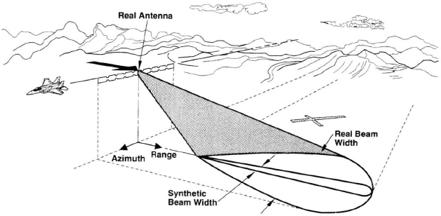
Figure 11.4 SAR image formation explained using antenna theory.

Synthetic array azimuth resolution is twice that of a real array with the same aperture length. A real array has both a one-way and a two-way radiation pattern. The one-way pattern is formed upon transmission as a result of the progressive difference in the distances from successive array elements to any point off the boresight line. This pattern has a sin x/x shape when amplitude weighting is not utilized. The two-way pattern is formed upon reception, through the same mechanism. Since the phase shifts are the same for both transmission and reception, the two-way pattern is essentially a compounding of the one-way pattern and therefore has a (sin x/x)² shape. A synthetic array, on the other hand, has only a two-way pattern because the array is synthesized out of the returns received by the real antenna, which sequentially assumes the role of successive array elements. Since each element receives only the returns from its own transmissions, the element-to-element phase shifts in the returns received from a given point off the boresight line correspond to the differences in the round-trip distances from the individual elements to the point and back. This is equivalent to saying that the two-way pattern of the synthetic array has the same shape as the one-way pattern of the real array of twice the length, sin 2x/2x. Since antenna beam width is inversely proportional to array length, the synthetic array azimuth resolution is twice that of the real array.

In practice, SAR azimuth linear resolution d_A, is very often limited by fluctuations in aircraft velocity. These fluctuations cause errors in the placement of the radiator at its successive positions where radar transmission occurs as the array is generated synthetically. These errors constitute a deterioration of the synthetic antenna pattern; that is, they introduce random phase errors in the array gradient. This is exactly analogous to phase errors in real arrays due to errors in location of the array elements or the phases of the signals fed to them. Just as with a real array, the larger the synthetic aperture, the larger the phase-gradient errors—and the more difficult they are to control. Another practical limitation is the stability of the atmosphere between the array and the targets. Turbulence in the atmosphere introduces optical path difference fluctuations between the target and the aircraft antenna at its successive array positions; this produces errors in the phase gradient of the array. Again, these errors increase in a random-walk manner with increasing aperture length, and impose a limit on the maximum useful aperture length.

Aside from these practical limits to synthetic aperture length, there are theoretical limits to the azimuth resolution that can be obtained. Doppler frequency-filtering theory is useful in explaining unfocused SAR and focused SAR resolutions. First, observe that if the SAR radar is carried on an aircraft that has constant velocity, radar return from each angular direction, on each side of the velocity vector, will have a unique Doppler frequency shift. If a narrow bandpass filter is used to process the ground return, only reflections from scatterers within a narrow angular increment in azimuth will contribute to the output. Thus, the SAR radar acts as if it had a very narrow beam-width antenna pointing in a direction corresponding to targets with Doppler shift equal to the frequency of the band center of the bandpass filter. Second, by moving the filter band center frequency from zero Doppler frequency shift to maximum positive and negative Doppler shifts, the synthetic antenna beam can be scanned over a 180° arc on one side of the ground track. (See also Doppler theory in Chapter 10.) By repeating the process on the other side of the ground track, it is possible to look in all azimuth directions. Third, by using a bank of narrow-bandpass filters, one can get the equivalent of a simultaneous array of contiguous azimuth antenna beams that create a complete high-resolution image of a ground range bin without scanning. Forming simultaneous Doppler filter banks for several contiguous range bins creates the complete SAR image.

Synthetic aperture radars are characterized as either focused or unfocused systems. If the SAR Doppler filter banks are not tuned to the Doppler filter frequency of the desired imaging ground area continuously throughout the SAR array time, the system is said to be unfocused. When the SAR Doppler filter banks are continuously tuned, the system is focused. The process of tuning is called SAR motion compensation.

11.4.1 Unfocused Systems

The azimuth and range resolutions of an unfocused system are determined by the length of time a ground point's radar return remains in a range/Doppler resolution cell. Consider azimuth resolution first. If a strong ground target's radar return drifts from one Doppler filter to another due to its changing Doppler frequency during the SAR array time, part of its energy will be processed in one Doppler filter and part in another. Thus, the SAR image will show a bright spot in two contiguous Doppler filters and SAR azimuth resolution will be degraded. Thus, unfocused SAR azimuth resolution is defined by the change in Doppler frequency to the desired ground point during the SAR array time.

As an aircraft moves, the Doppler frequency shift of a given ground point P_T is not constant since its azimuth angle changes. During a time period ΔT_A, the azimuth angle to ground point P_T will change by Δθ due to the aircraft motion. The time required for the azimuth angle to a ground point at range R to change by Δθ degrees is

where V is the aircraft velocity and θ is the azimuth angle between the aircraft velocity vector and the line-of-sight vector to the ground point P_T.

The corresponding Doppler-frequency change is

where λ is the radar transmission wavelength.

The SAR Doppler filter bank passbands must have Δf_d Hz width if the ground point's return is to stay in their passband during coherent integration. The SAR array time T_A is the reciprocal of the Doppler filter passband Δf_d. Therefore, the array time is

To a first order, a good radar image will be formed as long as the ground return stays in a single Doppler filter during the coherent integration time. Thus, ΔT_A must equal T_A. Equating 11.1 and 11.3 and solving for Δθ obtains

for the azimuth angular resolution. The linear azimuth resolution is obtained by multiplying Δθ by R. This yields

for the linear azimuth resolution.

So far, our definition of azimuth resolution has been coarse. A refined definition of azimuth resolution is the linear extent of the SAR Doppler filter's 3-dB frequency width when the coherent integration time is chosen to maximize the radar return energy in a resolution cell. This optimal SAR array time is

and the resolution corresponding to this array length is approximately

Now, consider range resolution of an unfocused SAR radar. Unless compensated, aircraft motion toward the imaged ground point P_T will cause the radar return to move from one range cell to another. The time ΔT_r required for a ground element to move one SAR range bin of width d_r is

This restricts the maximum length of the synthetic array to

and the minimum synthetic array beam width to

Modern SAR radars compensate for this range-walk phenomenon. One implementation progressively delays the start of analog-to-digital converter (ADC) range sampling from pulse to pulse by a time delay amount equal to the product of line-of-sight velocity divided by PRF.

Early SAR systems were employed to generate synthetic aperture strip maps for the reconnaissance mission. The radar antenna beam was pointed orthogonal to the flight path as shown in Figure 11.4, and the aircraft was required to fly straight and level during data collection. Radar returns were stored in a tape recorder and processed on the ground by an optical correlator to create an unfocused SAR strip map image [1]. Range walk was not compensated.

11.4.2 Focused Systems

If the center frequency of a Doppler filter is shifted to track the changing Doppler frequency of a ground point P_T, a focused SAR image is created. SAR array time is limited only by the time the target is in the antenna beam of the physical antenna carried by the aircraft. The maximum length of the synthetic aperture D_SAR is then

where D is the physical (real) length of the aircraft antenna and θ_HP is its physical (real) beam width. Then the azimuth angular resolution of the focused radar is

and the linear azimuthal resolution at range R

This result asserts that the linear azimuthal resolution of a focused synthetic aperture radar is not a function of operating wavelength, range to the identification point, or the angle to the identification point with respect to the velocity vector. Furthermore, in order to increase resolution, the aircraft antenna must be made smaller. Of course, in practice, there are limitations imposed by the problems of keeping the synthetic antenna “straight” and by atmospheric “seeing” conditions.

Another limitation is the motion of the target element out of its original range bin, just as in an unfocused system. This occurs when

or

When this occurs, one reverts to Equation 11.8 to find Δθ:

Again, modern SAR radars compensate for this range-walk phenomenon.

The limiting resolutions set by Equations 11.12 and 11.15 are much more likely to be reached in a focused system than in an unfocused one, because d_r must be made quite small to equal the linear azimuthal resolution developed in the first case. Relative to antenna theory, the operation of focusing is equivalent to physically bending the synthetic array aperture so that its focal length is equal to the range to the identification point—hence the name. The theory of focused antennas is well developed [8].

The azimuth resolutions realized by a real beam (RBGM) radar, an unfocused SAR radar, and a focused SAR radar are compared in Figure 11.5. Each radar is assumed to transmit a 0.1-ft wavelength (X-band) pulse train through a 10-ft long real antenna aperture. Note that the azimuth resolutions of the RBGM and unfocused SAR radars are range variable, while the focused SAR resolution is constant. This very desirable resolution property is achieved through motion compensation.

Figure 11.5 Real beam, unfocused SAR, and focused SAR azimuth resolution comparison.

11.4.3 Motion Compensation

Modern synthetic array radars employ motion compensation techniques to create focused radar images during times of aircraft maneuver. SAR beams are focused relative to fixed ground points illuminated by the real antenna beam by subtracting the phase shift due to antenna phase center spatial motion with respect to the fixed ground point from each complex-valued sample of radar return. Each range/Doppler cell has a different Doppler frequency history since the line-of-sight angles to each cell are unique. Thus, the optimum motion compensation approach is to compute and apply a unique phase correction history for each resolution cell. However, this mechanization would be prohibitive to implement from a required processor throughput point of view. Fortunately, several cells, termed the depth of focus, can use a common phase correction history.

Two signal-processing formats have been created to generate SAR images: rectangular and polar. The rectangular format is based upon the assumption that the loci of points of constant range on the ground are orthogonal to the loci of points of constant Doppler frequency on the ground. In this case, geometric distortion caused by SAR image creation in the range/Doppler domain is minimal.

The polar format is based upon the assumption that radar returns are actually collected at equally spaced angle increments from a constant range. First, stored radar returns must be resampled to convert from polar format to rectangular format. Then two-dimensional fast Fourier transforms (FFTs) are formed to generate the SAR image. Due to its added complexity, polar format is utilized only for very fine resolution SAR image applications where geometric distortion in rectangular format is severe. For the remainder of this chapter, the rectangular format will be assumed.

Two methods of motion compensation have also been developed. Originally, motion compensation was performed entirely based on on-board inertial sensors that measured the antenna's spatial motion during the SAR coherent processing interval. The radar data processor utilized INS acceleration and attitude vector measurements to compute the line-of-sight phase history for SAR motion compensation. Then, the stored raw radar return was retrieved and the phase history subtracted from the radar return on a pulse-to-pulse basis. Finally, range bin and Doppler filter FFT's were formed sequentially to generate the SAR image.

In the early 1980s, INS technology could not provide the velocity and angular accuracies needed for motion compensation of very fine resolution SAR images. Therefore, the idea of utilizing the actual radar return to compute motion compensation phase histories was explored. This adaptive process has been termed autofocus. Algorithms to focus fine resolution SAR images both with prominent discrete radar returns and with only diffuse terrain have now been successfully developed. Autofocus is based on a three step logic: First, the radar forms one or more coarse resolution SAR images utilizing motion compensation data generated from the aircraft's master INS, which may be very remote from the antenna phase center. During this step, the original unprocessed radar returns are not destroyed but are stored in radar processor memory for the final processing step. Extra processor memory is required to store the results of the first step. Second, the coarse image(s) are analyzed to either select a prominent point target, whose stored phase history will be utilized to compute a motion compensation vernier, or to compute the Doppler frequency drift of a visible geometric formation from image to image. Third, the raw radar return data are retrieved, a refined motion compensation correction is applied, and the final SAR image is formed. A generic autofocus functional diagram is given in Figure 11.6.

Since most multimode radars utilized rectangular format to create SAR images, SAR signal-processing will be illustrated for this format. Synthesis of a signal-processing architecture for generating minimum-time SAR images during aircraft maneuvers involves a division of the radar ground return into range/Doppler cells that can be focused by a single-point motion compensation correction. For the range dimension, it is convenient to divide the range swath into zones, whose widths are fixed at a value less than the smallest expected range depth of focus. Signal-processing time will not be adversely affected by a conservative choice for range zone width, say, 16 range bins. The cross-range swath illuminated by the antenna is divided into zones whose widths are less than the computed azimuth depth of focus. Since signal-processing time will increase in direct proportion to the number of azimuth zones, azimuth depth of focus will be computed each array to select the minimum number of required azimuth zones.

Figure 11.6 Autofocus motion compensation utilizing radar return.

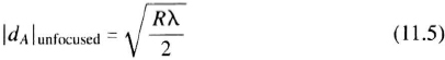
The signal-processing steps required to form a SAR image are shown in Figure 11.7. The signal processor compensates the phase of the nth radar return pulse, kth range zone after the Nth INS measurement by a correction ϕ(n, k) that is the sum of the patch center correction, and a range-dependent vernier correction.

The patch center correction is computed using a second-order Taylor series approximation of the patch center phase history. Line-of-sight velocity and acceleration values derived from INS data form the Taylor series coefficients. The range-dependent vernier correction is computed using a first-order gradient vector of Doppler frequency with respect to slant range vector.

After range-dependent phase correction, the radar return is processed through an azimuth prefilter and range compressed. Processing is performed in real time up to this stage. Range-compressed data are stored in processor memory until all the pulses required to form the SAR azimuth resolution cell have been collected. During the data collection period, an azimuth-dependent vernier correction is computed using a second-order Taylor series approximation of patch center phase history. Line-of-sight velocity and acceleration values derived from INS data are used as the Taylor series coefficients. Motion compensation data are stored in processor memory.

When all the radar pulses have been collected, the azimuth depth-of-focus is computed, and the number of azimuth zones with a constant motion compensation correction N_AZ are determined. Then the azimuth-dependent phase correction, azimuth compression, and subpatch selection functions are exercised N_AZ times. During the jth iteration, an azimuth-dependent phase correction q_A(j) will be applied to the range compressed data. The azimuth cells that are focused by q_A(j) will be selected after azimuth compression and magnitude detection will be performed. Then multilook image integration and the formatting for the display are accomplished.

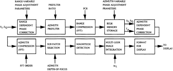
Figure 11.7 Signal-processing functional diagram.

TABLE 11.2 Motion compensation error budget

The ability of this motion compensation scheme to form focused SAR images is directly dependent on the quality and timeliness of INS data. Typically, the motion compensation design criterion is less than 90 deg (0.25 wavelengths) of quadratic phase error during a SAR array time. This criterion results in less than 10% broadening of the Doppler filter width (azimuth resolution degradation). Table 11.2 is a motion compensation error budget example. Phase error is computed for a 1.8 sec SAR array time (T_A).

11.5 PRECISION VELOCITY UPDATE

Determination of ownship velocity is obviously an important concern in the navigation of any airborne vehicle. For military aircraft, especially those employing radar air-to-ground modes, precise determination of ownship velocity often makes the difference between mission success and failure. For example, SAR images of the ground are often de-focused by ownship velocity error, and shifted in a way that can destroy their utility as targeting tools; Doppler-based techniques to estimate the velocity of ground-moving vehicles are rendered futile if the error in knowledge of the radar velocity vector is comparable to the speeds of the vehicles being tracked; miss-distances of ballistic munitions are enlarged by velocity error at the time of weapon release. Fortunately, air-to-ground radars, using the precision velocity update (PVU) mode, can measure the error in the vehicle's estimate of its own velocity and, thus, enhance their own performance. Typically, radar-derived corrections to the velocity vector, supplied by the inertial navigation system, are fed back to the integrators within that device. If velocity error feedback to the INS is not an option, a feed-forward mechanization, in which the radar accumulates velocity vector corrections over time, may be used.

Radar measurements of aircraft velocity exploit the Doppler principle to obtain projections of the velocity vector on chosen lines of sight (See Chapter 10, section 10.1.2). Using boresight directions that span 3-dimensional space and intersect the ground, one can solve for the components of the velocity vector in some reference axis set, e.g., a local-level North-East-Down frame. Since the Doppler frequency shift on an electromagnetic pulse that is sent and received by an emitter, and reflected from a stationary reflector, is (2/λ) times the radial velocity of the emitter in the direction of the reflection point, the relationship of aircraft velocity to Doppler measurements can be written:

The vector V is the unknown aircraft velocity vector, the vector L is an arbitrarily chosen unit line of sight (LOS) intersecting the ground, and the scalar f_D is the ground clutter Doppler measurement. If three independent lines of sight are chosen and the measurements are made so rapidly that the velocity vector is effectively constant during that time, then it is possible to solve for the three components of the velocity vector by inverting the matrix equation

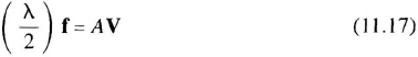
in which f is a triplet (f₁, f₂, f₃) of ground clutter Doppler measurements and the 3 × 3 matrix A has as its jth row (j = 1, 2, 3) the unit boresight line of sight (referred to the same axis set as V) associated with the jth Doppler measurement. Given the independence of the rows of A, the components of V are obtained by inverting A:

11.5.1 PVU Mechanization

Unlike the dedicated Doppler radars described in Chapter 10, where a bottom-mounted antenna is used to provide the measurement of the Doppler shifts, along three or four forward- and rearward-looking (Janus) and typically fixed beams, a multimode radar, either nose- or side-mounted, can be commanded to generate beams along almost any desired directions. In nose-mounted radars, these beams will, of course, be pointed only in the forward direction (non-Janus). The Janus and non-Janus effects on Doppler velocity accuracy are discussed in Section 10.1.2.

In the PVU mode of a multimode radar, the quantity measured is the difference between the Doppler shift predicted by use of the velocity vector supplied by the on-board INS and that associated with the true aircraft velocity. This difference, together with the line-of-sight information, is then sent to a navigation Kalman filter, usually residing in the INS, for estimation of the error in the velocity vector supplied by the INS. Instead of processing a triplet of measurements at a time, updates are performed, in turn, for each commanded line of sight. This approach obviates the need for rapidity in making the sequence of measurements along three lines of sight; V can change appreciably between measurements. The technique is based on the usually well-founded assumption that the velocity error vector is slowly varying. Figure 11.8 shows the functional mechanization of a typical PVU mode of a multimode radar.

The mechanization commits to hardware the task of referencing the radar returns to a frequency equal to the sum of the carrier frequency and a Doppler shift that is consistent with the current aircraft velocity and a commanded antenna LOS. The radar's variable frequency oscillator (VFO) is set to the frequency value given by 2/λ times the projection of the INS velocity estimate on the commanded antenna LOS. Radar processing is such that, if the INS velocity is exact, and the commanded LOS is achieved exactly by the antenna boresight, then the radar return from the groundpoint where the boresight intersects the ground will have been shifted to zero Hz. Any departure from this value is evidence of error in the INS velocity, the achieved antenna beam boresight, or both.

An essential feature of PVU radar data processing is that it determines the range/Doppler cell corresponding to the antenna beam boresight direction that was actually achieved (as opposed to the one commanded). Typically, this is done in a sequential manner. First, using main/guard sum channel data, a coarse estimate of beam boresight range is obtained by a sliding-window technique that finds the contiguous region containing the strongest returns; this estimate is then refined by averaging the values of elevation null returned by monopulse discriminants in a set of range-bins surrounding the coarse range estimate. Then, in a narrow swath surrounding the range associated with the newly found elevation boresight, the achieved azimuth is determined by averaging the values of azimuth null delivered by azimuth monopulse discriminants; the PVU measurement is taken to be the Doppler value associated with that cell. Discriminant techniques based on difference-to-sum ratios have the virtue that they are relatively immune to reflectivity differences in the area illuminated by the beam.

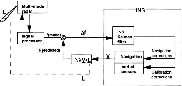
Figure 11.8 Block diagram of PVU mode.

Since the Doppler observations are inevitably noisy, a method of filtering is needed. Typically, at each beam position, the Doppler measurement is taken to be the average of N, approximately 6, independent measurements taken in quick succession. In the absence of information regarding the slope and nonuniformity of the terrain, the clutter return is regarded as coming from the intersection of the radar beam and a horizontal surface. The shape of the clutter spectrum (intensity versus Doppler) is a function of the illumination pattern delivered by the radar beam.

11.5.2 PVU Measurement Errors

The quantity measured by the radar in the PVU mode is the difference Δf between anticipated and measured Doppler frequency along a commanded antenna line of sight:

where f_true is the actual Doppler frequency of the radar return along the antenna beam boresight, and f_VFO is the Doppler value set in the VFO. Those quantities are related to velocity and line of sight through

The difference between the anticipated Doppler value (f_VFO) and the Doppler actually measured (f_true) is related to the following system error vectors: (1) the current error (ΔV) in the INS velocity vector and (2) the error (ΔL) in the achieved line of sight (i.e., the difference between the commanded LOS, whose calculation was based on estimates of heading, pitch, and roll supplied by the INS, and the LOS actually achieved by the antenna boresight):

where

Equation 11.22 shows that the measured Doppler difference contains not only the desired projection of the current velocity error on a chosen line of sight but also contains a term given by the projection of the full INS velocity vector on the boresight pointing error.

Failure to take explicit account of the last term (V_INS · ΔL) in equation 11.22 leads to a biased estimate of the actual velocity error; as an example, for an aircraft traveling at 300 meters/sec, every milliradian of boresight pointing error contributes an unmodeled velocity error of 0.3 meter/sec. Military aircraft often rely on velocity estimation accuracy of 0.2 meter/sec or better. Boresight pointing errors arise from several sources, including (1) INS attitude, (2) knowledge of the relative orientation of the INS case and the radar antenna base, (3) antenna gimbal readout errors affecting the antenna control algorithm, (4) electrical boresight, and (5) compensation for radome refraction. The dominant errors can usually be modeled as biases in some coordinate frame, and are thus well-suited to Kalman filter estimation. PVU-derived velocity estimation accuracy better than 0.25 meter/sec (1-sigma) is typical for some tactical aircraft equipped with medium-accuracy navigators whose unaided performance is 0.8 meter/sec (1-sigma), approximately. Achieving this at speeds approaching Mach 1 calls for antenna pointing error calibration accuracy considerably better than 1 mrad.

Equation 11.22 can be rewritten to show explicitly the dependence of the PVU measurement on the contributors to antenna beam-pointing errors listed above. The error ΔL can be written in the form of a vector cross product:

where Δθ is some triplet of small angle errors, and for brevity L_c is used to denote L_commanded. Equation 11.22 can then be made to read

or

The vector quantity Δθ can be written as a sum of angle errors resident in different frames; for example,

where Δϕ_INS is the vector of small errors (referred to the navigation frame) in the INS estimate of its own attitude; Δϕ_B is the triplet of small-angle errors (referred to the aircraft body frame) describing the uncompensated misalignment of the antenna base with respect to the INS case; Δϕ_A denotes the three small errors in the antenna gimbal readouts (roll, elevation, azimuth, in some sequence).

C_NB and C_BA are 3 × 3 orthogonal matrices; C_NB transforms vectors defined in the aircraft body frame into their representations in the navigation (INS) frame, while C_BA transforms Δϕ_A elements to the aircraft body frame. C_NB appears in the output message of the INS or can be constructed from the heading, pitch and roll angles in that message. The matrix C_BA is constructed from the antenna roll, elevation, and azimuth angles that are commanded in order to achieve the two conditions: (1) alignment of the antenna face normal with the commanded line of sight and (2) having the elevation monopulse axis horizontal (the azimuth axis then lies in the vertical plane containing the line of sight).

11.5.3 PVU Kalman Filter

The inner products appearing in Equations 11.26 and 11.27 allow immediate writing of the Kalman filter measurement equation; it is

where the scalar Δf is the measured Doppler difference described above, x is the state vector in the INS Kalman filter, and H is the single-row measurement matrix. It is standard practice in INS software to use a formulation of the Kalman filter that has the vector of estimation errors (estimated whole value minus true) as the state vector. If the elements of x are ordered so that INS velocity errors ΔV, INS attitude errors Δϕ_INS, antenna-to-body misalignments Δϕ_B, and antenna gimbal angle errors Δϕ_A occupy the first 12 locations as follows:

where superscript T denotes transpose, then measurement sensitivities to the errors in x are given by the row-matrix H, where

with zeros in the locations beyond 12. Each of the items separated by commas in the preceding two equations is a three-element row vector.

The evolution of the estimation errors appearing in Equation 11.30 is defined through the transition matrix definition. ΔV and Δϕ_INS are propagated via standard navigation error differential equations. Δϕ_B is treated as a random bias, namely, as an unknown vector that is constant in the body frame. In the formulation described above, Δϕ_A is also treated as a random bias, a constant vector in the antenna face frame. Thus, only constant errors (readout errors that are independent of the actual value of the commanded angles) can be treated with this approach. Other antenna-resident errors can be pursued (e.g., angle-proportional or scale-factor errors) but only at the cost of introducing further complexity.

The noise term in Equation 11.29 can be regarded as being equivalent to a random angle jitter. Thus,

where ΔΘ_R is a random vector that includes the contributions of any and all noise sources in the data collection and processing; it would include I/Q calibration errors, numerical round-off errors, residual postcompensation radome correction errors, and many others. It is worth noting that the magnitude of the measurement noise varies with aircraft speed | V |. In practice, it would be modeled as a zero-mean process with standard deviation given by

where σ_jitter is a value (measured or assumed) for the standard deviation of the effective jitter.

When the antenna is electronically scanned, the mounting error Δϕ_B remains in the measurement equation; the gimbal readout errors disappear, of course. Electrical pointing errors specific to an ESA are so small that they can be ignored. The PVU measurement model is simpler. However, beam broadening, especially for large angles off the antenna face normal, often leads to reduced measurement accuracy, which can affect the rate of estimation convergence. Otherwise, the operation of the mode is the same as for the mechanically scanned antenna.

11.5.4 PVU Mode Observability Concerns

The PVU measurement model (Equations 11.26 and 11.27) assumes the Doppler difference measurement is a weighted sum of velocity and angle errors. The weights are functions of antenna line of sight, aircraft velocity vector, aircraft body attitude, and antenna face attitude with respect to aircraft body. To estimate and calibrate the individual errors, PVU measurements should be collected in such a way that those weights do not appear in fixed ratios; this avoids the condition in which certain errors appear in fixed combinations with others, with the result that isolation of individual errors becomes impossible. For example, if straight and level flying conditions are maintained during a sequence of PVU measurements, then the INS attitude error Δϕ_INS and the antenna mounting error Δϕ_B appear through their sum; that is the ratio of their weightings is 1:1, regardless of the chosen line of sight. Thus, some departures from level flight must be made in the course of forming measurements along various lines of sight. These maneuvers need not be severe; changes of 10° to 20° in pitch and roll are adequate. Similarly, in order to distinguish velocity error from angle errors, the relative values of the weights arising from inner products with L_c (velocity error) and V × L_c (angle errors) must be made to change during the PVU measurement sequence. This can be done, for instance, by changing V, either through acceleration along track or by maneuvering. Similar concerns apply to ensuring observability of the antenna-resident errors Δϕ_A.

From a practical standpoint the decision to augment the state-vector of an INS Kalman filter with radar-specific states (e.g., Δϕ_B and ΔΦ_A above) is often problematic. The INS software design may not allow for easy insertion of new states or for the extra processing demands entailed. There is operational consolation in the fact that, if estimation of antenna-pointing errors is to work at all, it will converge in the first few minutes of the mission (over land) if the radar is dedicated to PVU operation during that time. The newly estimated antenna calibration corrections can then be stored for use in the antenna control function during the rest of the mission, and the angle-error states in the INS Kalman filter can be ignored.

11.6 TERRAIN FOLLOWING AND AVOIDANCE

The term terrain following refers to an aircraft maintaining a fixed height relative to the terrain immediately beneath it. Terrain avoidance and terrain clearance are related techniques, wherein terrain avoidance is performed for turn rates exceeding those normally performed during terrain following.

Figure 11.9 illustrates the geometry of the terrain-following process. The terrain-following system, comprised of airframe, flight control system, radar forward-looking sensor, radar altimeter, and pilot fail-safe monitoring, maintains the aircraft at the desired terrain following height, h₀. The forward-looking sensor measures the range R and angle β to the terrain. Angle β is measured relative to the radar antenna boresight, which in turn points at an angle α relative to horizontal during a terrain measurement interval. The terrain range and angle are then used to compute pitch (Γ, as defined in the figure) inputs to the flight control system that modify the aircraft trajectory to clear terrain at the desired clearance height h₀.

Figure 11.9 Terrain-following geometry.

The motivation for terrain following (TF) is based on terrain masking, reducing aircraft exposure to ground-based and airborne air defense systems. The degree of exposure reduction is a function of achieved terrain following height, terrain roughness, and system lookdown capability. Early applications of terrain following started in the 1960s with the U.S. Air Force F-lll and Navy A-6. Both the U.S. B-l A and B-1B aircraft support TF, with the latter being accomplished with a multimode radar interleaving other radar modes in between TF profile measurement intervals.

Figure 11.10 is a functional block diagram of a modern terrain following system. Starting from the left, terrain is sensed by the forward-looking radar, with enough range and angle coverage to clear the highest expected terrain at the desired clearance height. The radar processor generates a terrain profile consisting of elevation versus range, which forms the input to the pitch-command processor. The flight control system (FCS) accepts pitch commands and modifies the control surface positions. The system loop is closed when the radar collects a new terrain profile, which then generates a new set of pitch commands, different from the previous commands, since the aircraft is at a different position relative to the terrain. The altimeter acts as a check by comparing the distance of the terrain beneath the aircraft with the corresponding radar measurements. The forward looking infrared (FLIR) sensor provides backup data on the presence of wires, with the radar providing height information designed to fly over the tops of towers, thus avoiding the wires. The pilot's interface consists of the display, flight controls, and TF vertical acceleration switch for choosing smooth, medium, or hard ride quality. Pilot work load is intensive, with the requirement to perform a positive-pitch “pull-up” maneuver the instant an unsafe flight condition occurs.

Figure 11.10 Terrain-following functional block diagram.

Flight safety is the primary system design parameter being maximized, while minimizing radar on-time and power level. The latter is important for a low-observable aircraft. Flight safety requires embedding fail-safe features into system hardware, software, and interfaces such that the probability of an unsafe failure going undetected in an hour of TF flight is very small, 10⁻⁸ being a typical specification requirement.

11.6.1 Radar Mode and Scan Pattern Implementation

A TF sensor encounters a wide range of terrain backscatter values during routine operation. A flight profile over snow, desert, and military installations can easily encounter a dynamic range of 30 dB, as indicated in Chapter 10. In addition, discretes targets as large as 10⁴ meters² cross section may exist due to man-made structures acting as corner reflectors, or high radar-cross-section reflectors deployed as a countermeasure.

A terrain-following radar supports safe flight by scanning a volume containing the projection of the aircraft velocity vector onto the horizontal plane, defined as the ground track vector. Figure 11.11 depicts a nominal scan volume for level flight, with scan coverage equally split between the left and right sides of the ground track vector. The required extent of the scan volume in the horizontal dimension increases with uncertainty in either the velocity of the air mass or the aircraft with respect to an inertial navigation reference. The upper scan limit is a function of the expected highest terrain elevation, and the distance that elevation must be sensed for safe clearance, as indicated in Equation 11.34.

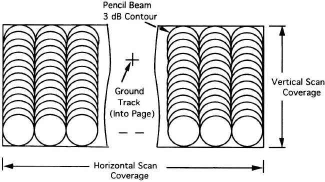
Figure 11.11 Terrain-following level flight scan coverage.

where

θu	is the elevation scan uplook
ΔZ	is the terrain clearance height above current altitude
VH	is the horizontal component of aircraft velocity
Tw	is the minimum time required to safely clear maximum terrain height

The aircraft flight time from the instant of sensing to the time the aircraft passes over the highest terrain point is defined as the warning time, T_W. As described later, during terrain-following operation, the aircraft flight control law is based on maintaining a constant horizontal velocity, and either a positive or negative vertical acceleration causing consecutive pull-up or push-over parabolic trajectories. Safe flight requires that pull-up and push-over trajectories intersect at no more than one point in space, where the slopes of the two parabolas are equal. Combining the equality of slopes with the definition of warning time results in a relationship between maximum terrain elevation ΔZ, warning time T_w, and the two vertical accelerations, as shown in Equation 11.35.

where

Ap	is the positive vertical acceleration
AN	is the negative vertical acceleration

Substituting this result for ΔZ in Equation 11.34 leads to a requirement for the upper elevation scan limit, θ_U.

A terrain-following radar performs terrain data collection over the scan volume appropriate for either level or turning flight. Scan implementation is a function of antenna beam width. For the case of a pencil beam, scanning is performed in vertical bars such that consecutive beam pointing angles within a bar have overlapping 3-dB contours, as indicated in Figure 11.11. This overlapping provides smoothed estimates of terrain SNR and height as a function of beam position. The beam selection logic then uses these data to select which beam positions to use within a range cell for final height estimates. This beam selection logic ensures safely measuring the tops of towers, and reduces upward biasing of rain, as indicated in Figures 11.12 and 11.13.

Figure 11.12 Beam selection logic for towers.

11.6.2 Terrain Measurement

Figure 11.14 depicts radar height estimate formation for a single-beam-pointing angle. The radar's video sampling interval and system bandwidth define the range cell.

The term centroid defines the angle, as observed from the radar and measured in a vertical plane, from the antenna boresight to the center of the range cell. The extent defines the angular width of the terrain within the range cell, measured in a vertical plane from the radar. If the extent were a fraction of a milliradian, then the terrain return due to a coherent radar pulse can be treated as being from a point target, and mutual interference from multiple scattering sources within the range cell, described by the term scintillation, would have negligible effect on centroid measurement. This point target assumption is invalid for most terrain conditions and practical range sampling intervals. Assuming an aircraft height of 200 ft, and 150-ft range cells, results in flat-terrain extents of 7.0 mr at 2000-ft slant range. In the worst case, scintillation could eliminate the effective radar cross section of all but the near-range scatterers within the range cell, causing an unsafe underestimation of terrain elevation by several milliradians. The effect is more pronounced (and unsafe) for terrain features with great vertical height, such as cliffs and towers. To obtain maximum radar illumination across the full elevation extent, the radar transmits over a wide bandwidth, either with sequential pulses at different frequencies or a single wideband pulse, whose returns are filtered independently using a digital or analog filter bank. Centroid and extent estimates are then made from these wideband radar returns.

Figure 11.13 Beam selection logic for terrain to avoid bias due to rain.

Figure 11.14 Terrain height measurement based on centroid and extent.

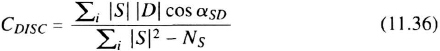
Elevation centroid and extent processing has been successfully applied in several terrain-following systems. The radar return from each range cell is processed using in-phase (I) and quadrature-phase (Q) samples from both sum and difference monopulse channels. Equation 11.36 shows the processing of sum and difference video signals to form a centroid discriminant, C_DISC, and Equation 11.37 shows the corresponding processing to form the extent discriminant, E_DISC.

where

|S|	is the magnitude of complex-valued sum channel video signal for ith frequency
|D|	is the magnitude of complex-valued difference channel video signal for ith frequency
αSD	is the phase angle between complex-valued sum and difference signals for ith frequency
Ns	is the sum channel noise power estimate
i	is the transmitted frequency channel number

where N_D is the difference channel noise power estimate.

These discriminants (C_DISC and E_DISC) are based on maximum-likelihood estimation, assuming a Swirling II fluctuation [18] model for terrain returns, and a Gaussian radar receiver noise model. As shown in Figure 11.15, the centroid and extent discriminants are coupled, deterministic functions of the ideal centroid and extent, due to the effective integration of sum and difference patterns across the terrain extent and the location of the terrain centroid relative to the difference channel null. A look-up table indexed on centroid and extent discriminant inputs performs the required inverse mapping. The final terrain elevation is formed by summing the centroid and half of the extent.

11.6.3 Aircraft Control

The terrain-following height control algorithm meets three basic requirements. First, the aircraft should clear terrain with negligible vertical velocity. Second, the autopilot should issue either a constant positive or constant negative vertical acceleration, relative to 1g, depending on terrain measurements. Third, the horizontal velocity should remain constant. As indicated in Figure 11.16, the combination of these requirements leads to the aircraft executing either a pull-up parabolic trajectory (corresponding to a positive vertical acceleration implemented by pitch-plane control surfaces) or a push-over parabolic trajectory (corresponding to a negative vertical acceleration).

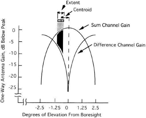
Figure 11.15 Terrain projected onto sum and difference gain patterns.

For a final step in terrain height measurement, the processing places pushover parabolas over each of the terrain profile range and elevation pairs. Whenever the aircraft is higher than the desired terrain following height, the control law continues to command a push-over maneuver, until the pull-up parabola is tangent to one of these push-over parabolas. Note that both pull-up and pushover parabolas are augmented by airframe-dependent climb and dive limits.

Figure 11.16 TF aircraft height control based on terrain heights.

11.7 MULTIMODE RADARS

Multimode radars perform a variety of functions using common hardware. The most prevalent examples are for military applications. Life-cycle cost economics has forced the military services to abandon their traditional approach of developing single mission aircraft, such as the F-14 and A-6, and concentrate instead on multimission aircraft, such as the F/A-18. A multimission aircraft radar's mode suite includes range-while-search, track-while-scan, single-target track, weapon support, weather avoidance, RBGM, SAR, fixed-target track, ground-moving target track, and terrain-following modes. In the multimission application, the radar is designed to provide the best balanced performance for all missions.

Traditionally, air-to-ground radar designers prefer high RF frequencies (Ku-band) that provide finer antenna azimuth resolution, given a fixed length aperture, and shorter SAR integration periods, given fixed range, speed, azimuth angle, and azimuth resolution. Low PRF wave forms are employed to yield range-unambiguous measurement of ground target location. In contrast, air-to-air radar designers select lower RF frequencies (X-band) to minimize atmospheric losses. High PRF wave forms are utilized to maximize average radiated energy and to provide velocity-unambiguous coverage. Ground return and approaching airborne targets, which are the most threatening, are separated in Doppler frequency when this wave form is employed. Medium PRF is also utilized to acquire and track airborne targets in a look-down engagement. Multimode radar designers must balance these two design preferences.

Multimode radars comprise an antenna, transmitter, receiver/exciter, and processor units. Power supply modules may be distributed among the functional units or packaged in their own unit. Antenna, transmitter, and exciter RF frequency choice is a compromise between the air-to-air and air-to-ground performance benefits gained at different extremes of the RF spectrum. Typically, a RF frequency band in the X-band regime is chosen. However, RF hardware technology advancements are focused on increasing RF bandwidth. In the twenty-first century multimode radars may possess RF bandwidths covering suitable portions of the X-band and Ku-band spectrums.

Air-to-air radar antennas are designed to yield maximum antenna gain, minimum beam width, and negligible sidelobe level. A “pencil” beam width is desired. Colocated guard horns are sometimes utilized for RFI elimination and ECCM purposes. Air-to-ground radar antennas are designed to provide uniform illumination of large ground swath over a range of depression angles. Typically, a large cosecant-squared elevation beam is employed. Sidelobe level is not as critical a design parameter. Monopulse or interferometer techniques are used to obtain azimuth target location information. A multimode radar antenna must possess all the properties of both designs. Basically, the multimode radar antenna is designed for the more stringent air-to-air application and has provisions to spoil its elevation beam when required for air-to-ground applications. Antenna elevation beam width has two values selectable by the radar processor.

Multimode radar transmitters and exciters must provide a large range of RF frequencies, pulse widths, and PRFs. Transition from one set of operating parameters to another must be rapid. The radiated RF wave form must be completely “programmable” by the radar processor. Power management of the transmitted energy is also desirable.

The receiver function must be “programmable” as well. A narrow bandwidth, large dynamic range receiver is required to support air-to-air modes, while a wide bandwidth, low dynamic range receiver is needed to support air-to-ground modes. The receiver must provide matched filtering for a variety of signal pulsewidths and PRF's. The analog-to-digital covnerter's precision and number of range samples taken each pulse repetition interval (PRI) must be selectable.

A multimode radar processor performs four functions, specifically, signal processing, data processing, radar units control, and system input/output management. All functions are completely defined and managed by software. A typical multimode radar software program comprises 100,000 to 200,000 instructions. Higher-order languages, such as JOVIAL and Ada, are employed for data processing, radar units control, and system input/output. Signal processing is accomplished through a structured software language. The hardware architecture comprises a cluster of signal-processing elements acting on radar return data in parallel, a cluster of data-processing elements partitioned to accomplish data processing, radar unit control, or system input/output, a large radar return data memory, and a large program memory. The number of processor modules depends on application.

11.8 SIGNAL PROCESSING

High-speed, software programmable signal processors are key to the implementation of multimode radars. Radar weight would be prohibitive, and aircraft power and cooling services could not support radar functioning if most radar signal conditioning and processing were not performed in a compact, lightweight special-purpose computer. SAR signal processing, which is illustrated in Figure 11.7, extracts radar imagery from the radar ground return. PVU signal processing, which is described in Section 11.5, extracts velocity vector error estimates from ground return. Terrain-following signal processing, which is defined in Equations 11.28 and 11.29, produces a terrain elevation angle profile versus range and isolates elevated point targets. Moving-target signal processing, which is discussed here, extracts target location information from the radar target return. These four signal-processing algorithms examine different portions of the radar Doppler frequency spectrum to perform their tasks.

Figure 11.17 is a generic functional block diagram for airborne or ground-moving target detection and location signal processing. This entire sequence of functions is implemented in software that is executed by parallel, “pipeline” processors. The execution of software modules is divided into three time-critical levels, namely, those computations that must be performed during a pulse repetition interval (PRI), those computations that must be performed during a coherent processing interval (CPI), and those computations that must be performed during an antenna dwell.

During a PRI, signal processing must compensate the range samples of azimuth difference channel and sum channel radar return for RF front-end imbalances, such as sum/difference phase/gain imbalance, and perform pulse compression. Each PRI pulse compressed range sample is stored in memory for later processing.

During a CPI, a fast Fourier transform (FFT) is utilized to form a Doppler filter bank spanning the PRF interval for each range bin and each radar channel of data. The resulting sum channel data grid is scanned to detect moving targets. A constant false alarm rate detector (CFAR) adapted to a noise probability density function (PDF) estimate is utilized to detect moving targets. Preliminary estimates of target range, Doppler frequency, and azimuth angle are formed for each potential detection and stored in processor memory.

If the radar wave forms are range and Doppler ambiguous, each potential target's range/Doppler measurement from each CPI must be expanded into the set of all possible unambiguous range/Doppler coordinates for the target on each CPI. The sets from all CPI's are compared during an antenna dwell to determine an unambiguous range/Doppler measurement.

11.9 AIRBORNE WEATHER RADAR

Any enterprise involving travel or navigation has to take account of the potentially catastrophic impact of adverse weather. Airborne radar is in some senses unique in its ability not only to make measurements (of ownship position, velocity and heading, etc.) that aid the navigation function but also to detect the presence and the features of weather formations. The radar observations involved in a weather mode are (1) magnitude detection of reflections from clouds and precipitation and (2) Doppler measurements of the motion of particles within a weather formation. Magnitude detection, accompanied by use of sophisticated reflectivity models, allows determination of particle type (rain, snow, hail, etc.) and precipitation rate. Doppler measurements, usually achieved by pulse-pair processing, can be made to yield estimates of turbulence intensity and wind speed. Reliable determination by airborne radar, of the presence and severity of the phenomenon known as wind shear, has been an important area of study in recent years.

Dedicated weather radars and multimode radars with a weather mode are usually nose mounted, and they include a weather display. Avoidance of hazardous weather conditions is the intent; however, in tactical aircraft the output of the weather mode is often used to adjust radiated power levels and processing thresholds for the presence of precipitation in the region between the radar and the target or area of interest. Typically, a real-beam map mode is employed, using a single value for elevation angle and scanning in azimuth. Radar returns are range gated and indexed by beam boresight angles. Processing is similar to that in which ground maps are formed but no attenuation is applied to the radar return, because of the relatively low reflectivity of clouds. The resulting display often shows weather formations in range (out to 100 km, approximately) and angle with respect to the aircraft nose, with indications of precipitation and hazard levels.

Figure 11.17 Generic moving target detection signal processing.

11.9.1 Radar Reflectivity of Weather Formations

The radar reflectivity of weather formations depends strongly on the precipitation type (rain, snow, hail, etc.), on the precipitation rate, and on the carrier wavelength. The radar cross section (RCS) of an individual droplet is well approximated by [19]

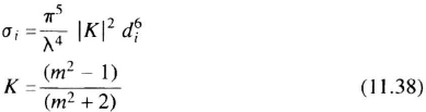
where d_i is the diameter of the droplet and m is the complex index of refraction. For microwave radar wavelengths, |K|² has the value 0.93 for raindrops and 0.2 for ice crystals and snow [19]. Summation of the σ_i over a unit volume of the cloud gives the RCS (per unit volume) for the precipitation:

Knowing the distribution of particle sizes for a given precipitation type and rate allows calculation of reflectivity after determining the value Z of the summation in Equation 11.39. Z has been determined experimentally for many conditions; Figure 11.18 shows a log–log plot of RCS (m² per cubic meter) versus precipitation rate (mm per hour), for rain and snow, with carrier wavelength as parameter. Most airborne weather radars operate in either C- or X-band. The λ⁻⁴ dependence of reflectivity on carrier wavelength favors X-band radars for this task.

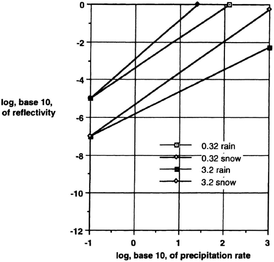
Figure 11.18 Log–log plot of reflectivity (meter²/meter³) versus precipitation rate (mm/hr).

11.9.2 Weather Radar Processing

Figure 11.19 depicts the processing stages involved in using radar data to detect weather formations and to measure precipitation rates and air-movement conditions. Frequency agility is used to minimize range ambiguities. The sequence (upper path in the figure) by which the presence of a given weather state is inferred from the magnitude of the radar return is (1) use the radar range equation to solve for the RCS η, after accounting for range and for parameters specific to the radar set (transmit power, antenna gain, etc.), (2) choose a value for |K|² that is consistent with some precipitation type (e.g., snow) and solve for Z, (3) knowing Z, use a look-up table or formula to infer the precipitation rate, (4) repeat (2) and (3) for any other precipitation types that may be present.

Determination of wind speeds within a weather formation has considerable safety value. Doppler-based processing can detect the presence of turbulence and provide a warning to the pilot if a pre-set safety level for wind speeds is exceeded. Even clear-air turbulence can be detected, despite the absence of a large mass of water molecules, if the sensitivity and transmit power are sufficient to deal with the low reflectivity levels provided by dust at low levels and sparsely distributed ice crystals at high altitude.

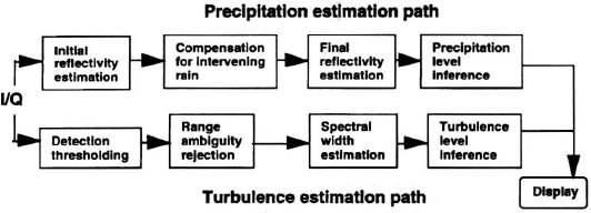
Figure 11.19 Weather mode radar processing for each range bin.

The lower path in Figure 11.19 shows the processing associated with measurement of air motion within a given volume. The pulse repetition frequency (PRF) is higher than that used in the upper path, in order to span the spectral width needed to represent faithfully the Doppler shifts of the radar returns. The spread of radial velocities within the air mass of interest is then calculated from the measured spectral width. Comparison with pre-stored values allows calculation of a safety index; for example, 5 meters/sec is often regarded as a threshold beyond which a turbulent air mass is regarded as posing a hazard for navigation. The mean velocity of mass within a given range-angle cell cannot easily be calculated without a moving target indicator (MTI) mode and accurate ownship velocity.

11.9.3 Radar Detection of Microburst and Wind Shear

Detection of microburst-induced wind shear has been a very active area of study in recent years. This phenomenon, involving strong downdrafts and high-velocity, horizontal airflow at low altitudes, is extremely hazardous to aircraft during landing and takeoff. Microbursts usually contain rain. The rapid transitions in lift conditions (see Figure 11.20) can confront the pilot with a life-or-death situation without enough reaction time to prevent disaster. As the aircraft approaches the center of the microburst, the outflow acts as a headwind. The pilot, after responding to an apparent condition of excessive lift, may suddenly find that there is not enough time or altitude in which to avert disaster in the reduced-lift conditions that rapidly occur, for the microburst outflow becomes a tailwind once the aircraft has passed through the center. There are plans to install radar wind-shear detection capability on all commercial airliners in the next few years.

Methods for radar detection of microbursts are based on recognition of air movement through Doppler processing. Some approaches attempt to detect the low-altitude, radial, horizontal airflow that accompanies them. Others key on detection of the fast downward movement of the vertical column of air and precipitation that characterizes a microburst. All have the objective of detecting those dangerous conditions at a range that allows enough time for evasive action.

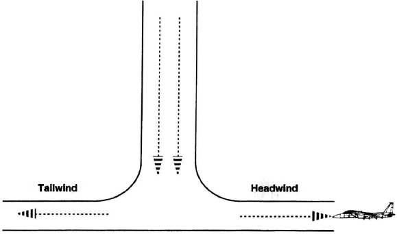
Figure 11.20 Microburst-induced wind shear which poses a hazard to aircraft at landing and takeoff by creating adjacent regions of opposite wind directions.

Devising a radar mode for wind-shear detection presents the designer with numerous trade-offs. For example, a high-carrier frequency is desirable in order to maximize radar reflectivity, which is proportional to λ⁻⁴; however, this choice (e.g., K_u-band) may reduce the performance of the long-range weather mode through increased atmopsheric attenuation. Another example relates to waveform selection. While medium PRF is best suited to detection of motion with velocities found in microbursts, range ambiguities with this wave form allow reflections from ground-moving vehicles (GMVs) to appear in the range bins of interest; this complicates the task of estimating air-mass velocities. Selection of a low PRF, such as 2 kHz, gives rejection of GMV returns through removal of range ambiguity but requires careful beam management in order to ensure that ground returns do not appear in the range interval of interest. Pulse compression selection poses another design decision—improved signal-to-noise ratio versus unwanted sidelobes.

11.10 FUTURE TRENDS

The first fifty years of radar history have witnessed dramatic technology advancements. Yet, greater advances are forecast for the future. The trend is toward a truly digital radar. Figure 11.21 illustrates the radar's progression from analog to digital technology. In the 1960s, radars employed analog technology almost exclusively. Analog-to-digital conversion (ADC) took place at the output of an analog crystal filter bank (after Doppler signal processing and target detection). Only elementary mode control logic, target tracking, and display formating were performed digitally. In the early 1980s, digital, programmable signal processors were introduced. The ADC function took place after receiver down conversion to an intermediate frequency, and all signal and data processing was performed digitally. The focus of the 1990s and in later years will be large-scale application of electronic scanned arrays, which will enable further progress toward a digital radar.

11.10.1 Electronic Scanned Arrays

A fundamental limitation in military radars is situation awareness. Mechanically scanned arrays are limited by inertia and cannot collect radar returns over several separated, spatial volumes quickly enough to provide current, accurate information to the pilot. This limitation is overcome by electronic scanned arrays (ESA's). In these, the antenna's beam is moved electronically by setting the phase angles of phase shifters located at each radiating element to provide a linear phase taper across the array surface. The slope of the phase taper determines the direction in which the antenna's beam will be pointed. Since the antenna's phase shifter settings can be changed in a few microseconds, an ESA's beam can be repositioned almost instantaneously. In addition, antenna reliability is dramatically improved, since ESA's have no mechanically moving parts, such as antenna gimbals, potentiometers, rotary joints, or hydraulic/electronic motors.

Two ESA technologies are being pursued. Active ESA's contain active components, such as transmission amplifiers, while passive ESA's do not. Active ESA's will be populated with radiation elements that contain individual transmitters and first stage receivers in addition to phase shifters. Gallium arsenide circuit technology will be utilized. The traditional single transmitter and a single mechanically scanned antenna unit will be replaced by a single active array antenna populated with thousands of small transmit/receive (T/R) modules. A typical airborne active array antenna could contain 1000 to 2000 T/R modules, each capable of transmitting 5 to 20 watts of power. Obviously, an active array radar will solve many of the reliability and maintainability problems experienced in conventional single transmitter radars due to TWT and power supply failures. 4 to 6% of the T/R modules could fail without noticeable degradation in antenna performance. Also, a new radar system control variable is introduced. Since the gain of each T/R module is controllable, active array radars will adaptively alter their transmit and/or receive antenna patterns to maximize system performance. No longer will a mechanical switch be required to provide a cosecant “fan” beam for air-to-ground operation. In the future, any number of antenna beam patterns will be generated and altered instantaneously. Active ESA's will inherently provide the radar with a digital front-end.

Figure 11.21 (a) 1960s radar functional diagram; (b) 1990s radar functional diagram; (c) 2000s digital radar functional diagram.

11.10.2 Radar Processing

In the early 1980s, high-speed, programmable processors with architectures optimized for the complex-valued signal processing required by radars were introduced. Airborne radars possessed 128 to 256 thousand words of memory, performed signal processing with 2 to 6 million complex operations per second throughput, and accomplished data processing with 300 to 600 thousand instructions per second throughput. As a result, a full spectrum of air-to-air and air-to-ground radar modes employed in multimode operation could be implemented cost-effectively in a single radar through software. Dramatic improvements in the packaging density, throughput, and memory of radar processors was achieved between 1985 and 1995. In 1996, it was not uncommon for production radars to possess 4 to 16 million words of memory, perform signal processing with 40 to 60 million complex operations per second (MCOPS) throughput, and accomplish data processing with 2 to 16 million instructions per second (MIPS) throughput. Sixteen-bit processor precision was standard. While computer capacity has been increasing, circuit packaging advances, such as multi-chip modules (MCM's), have allowed the processor's physical size to decrease. By the year 2000, processor memory capacity, signal processing throughput, and data processing throughput will increase by a factor of ten. Gallium arsenide circuit technology may be utilized to achieve throughput goals. Thirty two-bit or higher processor precision will become the industry standard. Fiber-optic interconnects among circuit packages on a module will offer a promising solution to the pin fanout problem attendant with advances in circuit dense packaging.

With the great computation power and memory capacity of future radars, adaptive signal- and data-processing algorithms will be implemented. For example, current airborne radars cancel ground return by computing its expected Doppler spread and range extent using INS and antenna pointing information, and blanking the appropriate range/Doppler cells. Each filter in a Doppler filter bank has the same frequency domain transfer function, which is selected a priori as the best balanced design for all missions. In the future, radars will have the capability to select adaptively, based on the radar return, the frequency domain transfer function of each Doppler filter to optimize performance relative to its position in the range/Doppler grid at the current instant in time. Thus, Doppler filters close to main-lobe clutter will have asymmetric transfer functions adaptively chosen to minimize clutter feedthrough, while Doppler filters in the “clear” region will have symmetric transfer functions adaptively chosen to minimize thermal noise feedthrough.

11.10.3 Radar Receiver/Exciter Function

In the next century, analog receiver and exciter functions will be replaced with digital equivalents to achieve a totally digital radar. With the rapid evolution toward very fast ADCs, it is possible that by that time, ADCs will be fast enough to sample RF signals above the Nyquist rate, though with low precision. Then it will be possible to incorporate ADCs in each active array T/R module, or sub-groupings of T/R modules. Thus, the radar system will reduce to two units: a “digital” active array antenna and a very high speed digital computer. The digital active array antenna will transmit the selected radar wave form in the desired spatial direction. Each T/R module will amplify the radar return it receives and convert the result into a digital format. The very high speed digital computer will receive the digital outputs from the T/R modules and synthesize digital antenna patterns, such as the classical sum channel, azimuth difference channel, elevation difference channel, and guard channel, each stabilized for aircraft motion. RF and IF signal shaping and filtering will be accomplished digitally. Finally, the very high speed digital computer will generate the transmission wave form and antenna pointing commands, detect targets and determine their locations, track targets, generate synthetic aperture radar (SAR) images, format them for display, perform navigation functions, and execute periodic built-in test (BIT).

One advantage of the digital implementation is that segments of the active array aperture can be controlled independently. Thus, a digital radar will be able to search several separate volumes of space with different RF wave forms simultaneously, though with less overall transmitted power and larger antenna beam width, since the subaperture sizes are smaller. Air-to-ground and air-to-air radar modes will run simultaneously.

11.10.4 Interfaces and Packaging

In the future, fiber optics will be a basic ingredient of the digital radar. High-speed, large bandwidth busses will be required to connect the very high speed computer with the digital radar's active array antenna (see also Chapter 15). Noise immunity (as well as weight) will be critical. Fiber optics appears to offer the best solution to this problem. An active array with a fiber-optics feed network will provide true time delay signal collection so that high-performance SAR resolution will not be degraded at large azimuth angles.

Smart skins is a future radar packaging concept that envisions radar components being a component of the aircraft structure. In the future, the conventional physical design using SEM-E modules housed in individual units will give way to conformal sheets of electronics that are “wall papered” to the back side of the aircraft's skin or onto a bulkhead.

11.10.5 Displays

Radar information will be displayed on color flat-panel displays in the future. Liquid-crystal display (LCD) technology is expected to dominate this application. Nevertheless, electroluminescent, plasma, and field-emitter display technologies are being pursued for possible future use.

PROBLEMS

11.1. Calculate the width of the Doppler spectrum of the coherent terrain return detected by a radar with a beamwidth of 0.05 rad, a beam direction of 30 deg with respect to the velocity vector, having a carrier frequency of 10 GHz, and moving 90 meter/sec parallel to the terrain.

Ans.: 150 Hz.

11.2. An airplane traveling at 100 meters/sec velocity parallel to the Earth commands its radar to form a SAR image of terrain at 100-km slant range and 60-deg azimuth angle relative to the velocity vector. The radar has 10-GHz carrier frequency and a 1-meter diameter antenna. What is the smallest unfocused azimuth resolution that can be achieved? If motion compensation is applied, what azimuth resolution will be realized?

Ans.: 60 meters, unfocused 0.5 meter, focused.

11.3. How long will a X-band radar traveling at 100 meter/sec velocity parallel to the Earth collect radar ground returns to form a 10-meter resolution SAR image of the terrain at 100-km slant range and 45-deg azimuth angle relative to the velocity vector?

Ans.: 7 sec.

11.4. Find the angular protusion of a hill through the clearance plane of a terrain avoidance radar when the linear protrusion of the hill through the clearance plane is 600 ft, the slant range to the hill is 3000 ft, and the radar measures an angle of 30 deg between the antenna boresight axis and the hill.

Ans.: 13 deg.

11.5. What is the aircraft clearance in Problem 11.4? Assume that the antenna boresight axis is horizontal.

Ans.: 2100 ft.

11.6. How much error will result if the slant range to a navigation fix point of 10 nmi is used as the ground range when the aircraft altitude is 30,400 ft?

Ans.: −1.8 nmi.