
10 Doppler and Altimeter Radars
10.1 DOPPLER RADARS
10.1.1 Functions and Applications
The primary function of a Doppler radar is to continuously determine the velocity vector of an aircraft with respect to the ground. If the measurement is made in, or has been converted to, an Earth-referenced coordinate frame and resolved about north and east, the velocity components can be integrated into distance traveled from a known point of departure and the aircraft's geodetic present position and course and distance to destination can be calculated. Thus, a Doppler radar can be the primary sensor of a dead reckoning navigation system or one of the sensors in a multisensor system. The velocity is determined by measuring the Doppler shift of microwave signals transmitted from the aircraft in several narrow beams pointed toward the surface at relatively steep angles, backscattered by the surface and received by the Doppler radar receiver.
A Doppler radar has the following advantages over other methods of velocity measurement or dead reckoning navigation:
- Velocity is measured with respect to the Earth's surface. This is in contrast to air data systems which measure velocity with respect to the air mass and to most terrestrial radio navigation systems in which velocity measurement is based on differencing of successive position measurements.
- It is self-contained, that is, it requires no ground-based stations or satellite transmitters.
- The airborne transmitter power requirements are extremely small, which leads to low weight, size and cost of equipment.
- Its radar beams are narrow and pointed toward the ground at steep angles, which leads to extremely low detectability.
- It is an all-weather systems, except in extreme conditions of rain.
- It operates over both land terrain and water (except for completely smooth water surfaces).
- Its average velocity information is extremely accurate.
- It is particularly suitable for the measurement of three-dimensional velocity and at low velocities, as required for helicopter navigation and hovering.
- International agreements are not required, since ground equipment is not needed.
- Pre-flight alignment and warm-up are not required.
The disadvantages of a Doppler radar are the following:
- For autonomous dead reckoning navigation, it requires an external airborne source of heading information, such as a gyro-magnetic compass, an attitude-heading reference system (AHRS), or an inertial platform.
- It requires either internal or external vertical reference information for conversion of its velocity information into an earth referenced coordinate frame; however, this vertical information need not be of high quality.
- Position information derived from Doppler radar dead reckoning degrades as the distance traveled increases.
- The instantaneous or short-term velocity information is not as accurate as the average or smoothed velocity. This difference is not significant for general navigation but may be significant for other applications.
- For over-water operation, accuracy is somewhat degraded due to backscattering characteristics and water motion.
The techniques of Doppler radar velocity measurement and navigation evolved from airborne radar development, notably airborne moving target indication, and from automatic dead reckoning navigation systems using airspeed meters. The earliest applications of Doppler radar were in military aircraft for dead reckoning navigation and weapon delivery. These systems have been installed in thousands of military aircraft of all major nations. Typical examples in the United States are the B-52, F-111, B-l A, E3A, P2V, P3V, S3A, E2A, and many thousands of helicopters. In the 1960s, the world's international commercial airlines began using Doppler radar systems for dead-reckoning navigation, primarily for over-ocean operations. These were interfaced with gyro-magnetic heading references and course line computers. In 1996, inertial and inertial-radio systems had replaced Doppler radars for that application.
Doppler radars have been used for the velocity measurement required for the soft landing of planetary and lunar space vehicles, such as the Surveyor and the Apollo Lunar Excursion Module (LEM).
In 1996, the most important wide use of Doppler radars was in various types of military helicopters, for such applications as navigation, hovering, sonar dropping, target handover for weapon delivery, and search and rescue. They have also been used on unmanned aerial vehicles (UAVs) and drones, as well as on military fixed-wing aircraft. By 1996, about 40,000 Doppler radars had been produced and deployed on aircraft worldwide.
In many aircraft, Doppler radars are employed in conjunction with inertial platforms, wherein the velocity data from the Doppler radar are used for damping of the inertial navigation system's Schuler oscillations (Sections 7.6.3 and 3.4). The difference in the characteristics of the velocity data from these two sensors, such as the small long-term velocity error of the Doppler radar and the small short-term velocity error of the inertial system, has lead to the desirability of combining the data from these two sensors in some form of optimum estimation filter (Chapter 3). Similarly, in some configurations Doppler radar velocity data are mixed with data from a position sensor, such as the Global Positioning System (GPS) receiver (Sections 10.1.5 and 3.8).
The Doppler radar velocity measurement function has been incorporated into coherent forward looking search and tracking radars for precision velocity update of the aircraft's inertial system: in 1996 this approach was used widely on high performance military aircraft (Section 11.5).
To accomplish dead-reckoning navigation by Doppler radar, a complete Doppler system needs to contain the functions shown in Figure 10.1. The Doppler radar measures the aircraft velocity with respect to its antenna frame coordinates. The heading reference and vertical reference, or a combined attitude and heading reference system (AHRS), or an inertial reference unit (Chapter 7) determines the direction of the aircraft antenna with respect to the horizontal plane and north. The navigation computer then resolves the aircraft velocity components obtained from the Doppler radar about the vertical and true north and continuously integrates the horizontal velocity components into distance traveled from the point of departure. The resulting present position can then be compared with destination coordinates to provide other desired navigational quantities, such as bearing and distance to destination, Figure 10.1.
10.1.2 Doppler Radar Principles and Design Approaches
The Doppler Effect Operation of a Doppler radar is based on the Doppler effect which was predicted in 1842 by the Austrian scientist Christian Doppler in connection with sound waves and was later found also to be exhibited by electromagnetic waves. The Doppler effect can be described as the change in observed frequency when there is relative motion between a transmitter and a receiver. Furthermore, this change in frequency, called the Doppler shift, is directly proportional to the relative speed between transmitter and receiver. In the case of electromagnetic waves (unlike the case of sound waves), it makes no difference in the proportionality relationship whether the transmitter, the receiver, or both, are moving. If the relative velocity of the transmitter and receiver is much smaller than the speed of light (as in the case of aircraft), the Doppler shift is expressed by
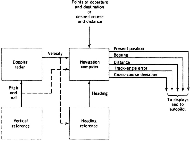
Figure 10.1 Doppler navigation system.
where
| v | is the Doppler shift |
| f | is the frequency of the transmission |
| c | is the speed of light |
| VR | is the relative velocity between transmitter and receiver |
| λ = c/f | is the wavelength of transmission |
From Equation 10.1 it is seen that, if the value of λ is known and v is measured, the relative velocity can be determined.
To measure the aircraft's velocity, a radar transmitter-receiver is mounted on the aircraft and radiates electromagnetic energy toward the Earth's surface by means of several beams, one of which is shown in Figure 10.2. Some of the energy is backscattered by the Earth and is received by the radar receiver on the aircraft. If the aircraft is moving with a total velocity V, the beam measures VR:
where γ is the angle between the direction of the velocity vector V and the direction of the beam centroid, and b is the unit vector along the beam centroid. VR is the component of relative aircraft velocity along the beam centroid. The factor 2 appears in Equation 10.2, since both the transmitter and the receiver are moving with respect to the Earth, from which the energy is backscattered. When Equation 10.2 is substituted into Equation 10.1, the following expression results:

Figure 10.2 Basic Doppler radar beam geometry.
Equation 10.3 is the fundamental expression for the measurement of velocity by means of a Doppler radar. It is also the basis for the operation of the synthetic aperture, Doppler beam sharpening, and precision velocity update (PVU) modes of airborne radars (Chapter 11). It states that each Doppler radar beam measures the component along the beam of the aircraft's velocity with respect to the Earth. Two faulty arguments have been advanced in the past which question whether proper operation of Doppler radar is possible—the smooth Earth paradox and the mountain paradox. The first paradox argues (falsely) that as an aircraft moves parallel to flat terrain at constant altitude, the range to the ground does not change and since there is no rate of closure (range rate) there can be no Doppler shift and Doppler radar operation is not possible at all. The second paradox argues (falsely) that if an aircraft is flying horizontally above upsloping terrain, its range to the ground along the beam continuously decreases and this range rate, with respect to the surface, gives rise to a significant error in velocity measurement. Both arguments are incorrect for essentially the same reason: the radar backscattering is produced by the discrete and irregular objects on the ground (pebbles, leaves, etc.) and there is indeed relative motion between the aircraft and each of these scatterers. If the surface were perfectly smooth, reflection at the surface would be specular and no reflected energy would reach the aircraft. Hence, if the scattering medium is sufficiently rough to give rise to a signal at the receiver, the signal will exhibit a Doppler shift according to Equation 10.3. Also, there is absolutely no error due to upsloping terrain (mountain paradox), since the backscattered signal comes from the individual, discrete, stationary objects on the ground and it therefore experiences the correct Doppler shift ([4] [40] [41]).
Since the three orthogonal components of velocity are of interest, a minimum of three noncoplanar beams are required to measure the three components. A beam configuration designed to accomplish this is shown in Figure 10.3. Since such a beam configuration has both forward- and rearward-looking beams, it is called a Janus configuration after the Roman god who had the ability to look backward as well as forward. In a Janus system, the Doppler shift obtained with, say, the right-forward beam can be subtracted from that obtained with the right-rearward beam in order to determine the heading velocity component VH. Since the forward-looking beam (beam 2 in Figure 10.3) gives rise to an increase in frequency (positive Doppler shift), and the rearward-looking beam (beam 1) gives rise to a decrease in frequency (negative Doppler shift), the subtraction process of the two Doppler shifts actually results in an addition process. For a condition of no drift, roll, or pitch, wherein the forward and rearward Doppler shifts are equal, the equation for the total Doppler shift from such a forward-rearward (Janus) pair of beams takes the form v = (4V/λ)cos γ. In typical microwave Doppler radars, the value of this Doppler shift is on the order of 30 Hz per knot of speed.
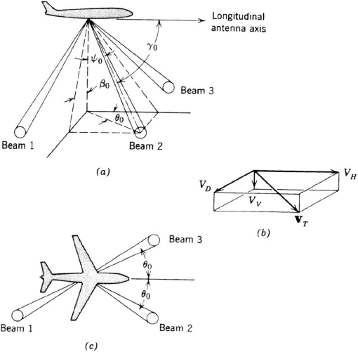
Figure 10.3 Three-beam lambda Doppler radar configuration.
The configuration shown in Figure 10.3 has been called a lambda-configuration, since the plan view of the beams has the form of the Greek letter λ, as seen from Figure 10.3c. The Doppler frequency in each of the beams is proportional to the algebraic sum of the projections of the three orthogonal velocity components along the beam. The mathematical expressions for the computation of the three orthogonal velocity components in aircraft coordinates are obtained from the beam direction cosines between the velocity components and the beam centroids and the addition or subtraction of the beam Doppler frequencies. For this particular (lambda-) configuration the beam Doppler frequencies are given by

where

From the above expressions the three orthogonal velocity components are

where
| is the along-heading velocity component, in aircraft coordinates | |
| is the cross-heading (drift) velocity component, in aircraft coordinates | |
| is the vertical velocity component, in aircraft coordinates | |
| vn | is the Doppler shift in beam n |
| α0 | is the depression angle of the beam centroids from the plane of the antenna, assumed equal for the three beams, ψ0 = 90° – α0 (Figure 10.3) |
| θ0 | is the azimuth angle of the antenna beams, that is, the acute angle between the projections of the longitudinal axis of the antenna and the antenna beam centroids on a ground plane parallel to the plane of the antenna, assumed equal for the three beams (Figure 10.3); the relationship among γ0, ϕ0, and θ0 is cos γ0 = sin ϕ0 cos θ0 |
| γH, γD, γv | are the angles between |
Although only three beams are required to provide the three components of velocity, most modern Doppler radars employ four beams, because planar array antennas naturally generate four such beams. The Doppler frequency of the fourth beam (v4) can be combined with v3 to obtain another estimate of ![]() (replace v2 and v1 in (10.4) and v3 and v4, respectively). The two estimates of
(replace v2 and v1 in (10.4) and v3 and v4, respectively). The two estimates of ![]() can then be averaged to obtain a more accurate value of this component. The difference of the two estimates of
can then be averaged to obtain a more accurate value of this component. The difference of the two estimates of ![]() should be very small; a large difference indicates that there is an error in the measurement of the Doppler frequency and hence that the Doppler velocity data are suspect and should not be used until the cause of this difference is corrected. This technique is used as part of the BITE (built-in-test equipment) of many Doppler radars. Similarly v4 can be combined with v1 to form another estimate of
should be very small; a large difference indicates that there is an error in the measurement of the Doppler frequency and hence that the Doppler velocity data are suspect and should not be used until the cause of this difference is corrected. This technique is used as part of the BITE (built-in-test equipment) of many Doppler radars. Similarly v4 can be combined with v1 to form another estimate of ![]() by replacing v2 and v3 in Equation 10.5 with and v1 and v4, respectively. Finally, v4 can be combined with v2 in Equation 10.6 (replace v1 and v3 with v2 and v4) to form a second estimate of
by replacing v2 and v3 in Equation 10.5 with and v1 and v4, respectively. Finally, v4 can be combined with v2 in Equation 10.6 (replace v1 and v3 with v2 and v4) to form a second estimate of ![]() . In each case the two estimates are averaged to obtain more accurate values of the respective velocity component. The fourth beam is thus redundent, since only three beams are needed to form a complete solution, as shown by Equations 10.4 to 10.6.)
. In each case the two estimates are averaged to obtain more accurate values of the respective velocity component. The fourth beam is thus redundent, since only three beams are needed to form a complete solution, as shown by Equations 10.4 to 10.6.)
In a fixed-antenna system, after ![]() ,
, ![]() , and
, and ![]() have been obtained, they must then be combined with pitch and roll information in order to generate the aircraft velocity components in Earth coordinates, VH, VD, and VV (as described later in this section). The total velocity vector magnitude V is the resultant of the three orthogonal components (Figure 10.3b). Hence, a Doppler radar with either a three- or four-beam configuration is capable of measuring the three velocity components and their sense of direciton.
have been obtained, they must then be combined with pitch and roll information in order to generate the aircraft velocity components in Earth coordinates, VH, VD, and VV (as described later in this section). The total velocity vector magnitude V is the resultant of the three orthogonal components (Figure 10.3b). Hence, a Doppler radar with either a three- or four-beam configuration is capable of measuring the three velocity components and their sense of direciton.
A variety of beam configurations have been used for Doppler radars, including Janus (two-way looking) and non-Janus (one-way looking) configurations. The Janus configuration has a very important advantage over a non-Janus configuration, namely a much lower sensitivity of velocity error to knowledge of the vertical attitude of the aircraft. Specifically, the expressions for the velocity error as a function of error in pitch angle for Janus and non-Janus systems, for a condition of no pitch, no drift, and no vertical velocity are as follows:
where
| εv | is the fractional horizontal velocity error |
| δV | is the absolute horizontal velocity error |
| δP | is the error in pitch angle |
Based on the conditions cited above, Equations 10.7 and 10.8 are equally applicable to fixed and physically stabilized antenna systems. From Equations 10.7 and 10.8, for a non-Janus system having a γ-angle of 70°, which is a reasonable value, the horizontal velocity error is 4.7% per degree of error in pitch angle, whereas for a Janus system the horizontal velocity error is only 0.014% per degree of error in pitch angle. Because of these considerations, all modern dedicated Doppler radar designs use some form of Janus configuration. However, when Doppler velocity is extracted from forward-looking search and mapping radars, a non-Janus configuration results (Chapter 11.5).
The choice of γ0 (nominal angle between antenna longitudinal axis and central beam direction) for a typical Doppler system represents a compromise between (1) high sensitivity to velocity (Hertz per knot) and overwater accuracy, which increases with smaller γ0-angles, and (2) high signal return over water, which increases for larger γ0-angles. Most equipments use a γ0 of somewhere between 65° and 80°. The choice of β0-angle depends on the desired sensitivity to drift (Hertz per degree), which tends to increase with increasing β0.
There are two different basic types of Doppler radar mechanizations that can be used for drift angle measurement. These are the fixed-antenna system, which is used in most modern systems, and the track-stabilized (drift-angle-stabilized) antenna system (Figure 10.4). Zero pitch and roll angles are assumed for the example in Figure 10.4. Figure 10.4a depicts a condition of no-drift angle (δ = 0) and no-climb angle so that the velocity vector V is located along the intersection of the local horizontal plane and the local vertical plane through the longitudinal axis of the aircraft. In other words, the aircraft flight is horizontal and the aircraft's ground track (or track) is the same as the aircraft heading. The hyperbolas in Figure 10.4, marked va, vb, vc, v−a, etc., are lines of constant Doppler shift, the positive subscripts representing positive Doppler shifts and the negative subscripts representing negative Doppler shifts. These hyperbolas, called isodops, are generated by the intersections of constant Doppler cones with an assumed flat Earth. In Figure 10.4a, it is clear that subtraction of the Doppler shifts from beams 1 and 2 will provide a measure of the along-heading velocity VH as given by Equation 10.4. Subtraction of the Doppler shifts from beams 2 and 3, as in Equation 10.5, will indicate a zero cross-heading-velocity component VD or a zero drift angle (since vb − vb = 0). Similarly, addition of the Doppler shifts of beams 2 and 3 will indicate a vertical velocity of zero. All of the ground intersections of the beams are located on the same equivalent isodops. Under drift conditions, as indicated in Figure 10.4b and 10.4c, the aircraft track direction is no longer coincident with the aircraft heading direction. If the antenna is fixed to the aircraft, a case depicted in Figure 10.4b, the beams will move with the aircraft, and the ground intersections of beams 1, 2, and 3 will be located on different isodops. Thus, subtraction of the Doppler shifts from beams 3 and 2 will indicate a nonzero cross-heading velocity as given by Equation 10.5; and subtraction of the Doppler shifts of beams 1 and 2 will determine the along-heading-velocity component, as given by Equation 10.4.
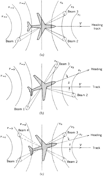
Figure 10.4 Comparison of fixed (heading-stabilized) and track-stabilized Doppler systems.
Operation of the track-stabilized antenna system concept, as used in earlier designs, is depicted in Figure 10.4c. In such a system, the difference between the Doppler shifts from beam pairs 1–3 and 2–A is used to drive a servo, which turns the antenna in azimuth until this difference is nulled. This occurs when the ground intersections of these beam pairs lie on the same isodop, thereby placing the antenna axis along the aircraft track. In these systems, Doppler signals from beam pairs 1–3 and 2–4 are typically obtained on a sequential basis and compared, thereby allowing the time sharing of receiving equipment. The drift angle can be read out directly as the angle between the antenna axis and the aircraft center line (e.g., from a synchro mounted on the antenna), and the ground speed can be obtained directly by averaging the Janus Doppler shifts from beam pairs 1–3 and 2–4. Since track angle is defined as heading angle plus drift angle, this system is also called a drift-angle-stabilized antenna system.
With regard to horizontal stabilization, two generic design approaches are possible (Figure 10.5). One uses an antenna fixed to the vehicle frame (Figure 10.5a) and the other uses a gimballed antenna that is physically stabilized to the local horizontal (Figure 10.5b). In 1996, the majority of dedicated Doppler radars configurations used the fixed-antenna approach. In this configuration, if the aircraft pitches or rolls, the antenna and hence the Doppler beam cluster center line will move with the vehicle, as shown by the dashed line in Figure 10.5a. To convert the velocity components from airframe coordinates ![]() ,
, ![]() , and
, and ![]() to the Earth-referenced coordinates needed for navigation, the former must be resolved about aircraft pitch angle P and roll angle R obtained from a vertical reference sensor (vertical gyro, AHRS, or INS). The conversion is given by
to the Earth-referenced coordinates needed for navigation, the former must be resolved about aircraft pitch angle P and roll angle R obtained from a vertical reference sensor (vertical gyro, AHRS, or INS). The conversion is given by

Figure 10.5 Doppler radar antenna geometry for fixed and attitude stabilized antennas.
where the velocity components are those defined in Figure 10.3.
The second type of Doppler radar is one whose antenna is continuously slaved to the local horizontal by means of the information from a vertical sensor. Although only a few Doppler radar designs employed this technique in 1996, it was used widely in previous years. Having computed VH, VD, and VV, from Equations 10.9–10.11, the drift angle can be obtained from the arctan (VD/VH) and the ground speed Vg from the magnitude of Vg:
The Doppler Spectrum Since each Doppler-radar antenna beam (Figures 10.2 and 10.3) has a finite beam width in the γ-direction, the return signal associated with the beam comes from a spread of γ-angles. Furthermore, the backscattering medium (the Earth) is composed of a multitude of randomly situated scattering centers, and the return signals from each have, in general, different amplitudes and different phases. In view of the frequency spread and randomness of the amplitude and phase of the scattering centers, the Doppler signal associated with each beam is in the form of a noiselike frequency spectrum (Figure 10.6). The spectrum is equivalent to band limited noise, the primary Doppler spectrum being superimposed on a substantially flat (uniform power spectral density) background noise. The shape of this spectrum is related to the antenna beam shape and is roughly Gaussian. The amplitude is a function of the radar parameters and the terrain backscattering coefficient in the radar-range equation discussed in Section 10.1.3. The amplitude modulation and the frequency modulation due to the scattering centers in the beam affect the shape and width of the spectrum. It is shown in the next section that amplitude effects are small, except at very low altitudes. The frequency characteristics will be considered further in the present discussion. The small spectra on each side of the main spectrum in Figure 10.6 represent energy returned by way of antenna side lobes. In typical systems, their level is so low that they are not sensed by the Doppler acquisition circuits; they are outside the frequency passband during Doppler tracking and therefore do not affect system performance.

Figure 10.6 Typical Doppler spectrum.
The Doppler frequency of interest, which is proportional to the velocity component along the particular beam centroid, is the mean or center of area of the Doppler frequency spectrum. It is this center of spectral power that defines the beam centroid for the velocity measurement.
The Doppler spectrum width is obtained, to a first approximation, by differentiation of Equation 10.3 with respect to γ and is given by the expression
where Δv is the half-power Doppler spectrum width and Δγ is the half-power two-way beam width of the antenna in the γ-direction. The approximations involved in the above expression for the spectrum width involve ignoring the differential effect of the inverse square law of the radar-range equation between the near and far regions of the illuminated area and assuming a constant backscattering coefficient of the target area. The former is a valid approximation for all practical Doppler radars, those using narrow two-way γ-beam widths, typically near 4 degrees. The latter is a good approximation for operation over typical land terrain. However, the scattering properties of water cause a change in the shape and average frequency of the spectrum, giving rise to an overwater calibration-shift error (see Section 10.1.4).
The relative (fractional) spectrum width is frequently of interest and is found by dividing Equation 10.13 by Equation 10.3; namely,
For typical practical Doppler radars. Δv/v ranges between 15% and 25%.
Because of the appreciable spectrum width, the instantaneous central frequency of the Doppler signal is subject to random fluctuations about its mean value, giving rise to a noise (or fluctuation) error in tracking the centroid and, hence, in velocity and distance measurement. A certain amount of smoothing time is therefore required to determine the velocity to a desired accuracy; that is, the accuracy of measurement increases with smoothing time. In general, it is necessary to select a velocity smoothing time whose value represents a compromise between velocity accuracy and the data rate required on the basis of system dynamics (e.g., the maximum acceleration of the vehicle). If too large a velocity smoothing time constant is selected, the Doppler radar will follow the vehicle accelerations with too great a lag. For the navigation problem the effective smoothing time for the average velocity or distance measurement is the total time flown. Hence, for the typical Doppler navigation problem, the fluctuation error due to this noiselike nature of the information is completely overshadowed by other errors after only a few miles of flight. (A quantitative discussion of this error is given in Section 10.1.4.) In multisensor navigation systems, such as Doppler-inertial systems (Chapter 3), the Doppler-radar information may be intentionally smoothed further, since the high-frequency information is supplied by the inertial sensor. It is the function of the frequency tracker to determine the mean or center of power of the Doppler spectrum, that is, to determine the single-frequency v that is proportional to the desired velocity component.
The Doppler correlation time τv is proportioanl to the reciprocal of the spectrum width Δv(τv ≈ 2/Δv). This is based on the fact that the power spectrum and the autocorrelation function are Fourier transforms of each other. The Doppler correlation time is the period during which the frequency and phase of the signal are invariant or predictable. At the end of this period the signal is nearly uncorrelated. This means that an independent Doppler measurement is made during each correlation time.
Scanning Noise At very low altitudes, there is a small amount of spectrum broadening due to amplitude modulation effects, over and above the basic spectrum width discussed above. This spectrum broadening has been called scanning noise, and the additional spectrum width is therefore called scanning noise spectrum. It will be shown that the effect is quite small in conventional Doppler radars, even at relatively low altitudes.
The time required for one set of scatterers that is illuminated by the entire beam intersection to be replaced by a new set is the scanning-noise correlation time of the signal τs. Twice the reciprocal of this time is approximately its frequency spectrum width Δvs. From the geometry of Figure 10.2, this correlation time τs is given by

where L is the diameter of the beam intersection and h is the altitude. Hence, the scanning noise spectrum width Δvs, is given by

The ratio of the scanning noise spectrum width and the basic spectrum width R is found to be

Substitution of practical values for the parameters shows that Δvs is insignificant except at very low altitudes. Because in an actual antenna the beam diameter in the near field (range is less than D2/λ, where D is antenna diameter) does not continue to decrease to a “point,” the scanning noise spectrum width does not continue to increase for altitudes below the extent of the near field. On the basis of conventional near-field antenna considerations, the scanning noise spectrum width will be just equal to twice the basic spectrum width at the altitude at which the antenna near field begins. This means that, in typical Doppler radars, R is never larger than 2 and that the total spectrum width is never larger than ![]() , even at extremely low altitudes.
, even at extremely low altitudes.
Operating Frequency In 1996, Doppler radars transmitted at a center frequency of 13.325 GHz in the internationally authorized band of 13.25 to 13.4 GHz. This frequency represents a good compromise between too low a frequency, resulting in low-velocity sensitivity (Hertz per knot) and large aircraft antenna sizes and beam widths, and too high a frequency, resulting in excessive absorption and backscattering effects of the atmosphere and precipitation. (Earlier Doppler radars operated in two somewhat lower frequency bands, i.e., centered at 8.8 and 9.8 GHz, respectively, but, in 1996, these bands were no longer used for stand-alone Doppler radars.)
Polarization The two types of polarization that have been used for Doppler radars are linear and circular odd (opposite rotation received). The latter has the advantage of efficient duplexing techniques. While circular even (same rotation received) has well-known rain discrimination characteristics, it suffers from an appreciable backscattering loss over water. In 1996, linear polarization was used.
Doppler Radar Functions A typical dedicated Doppler radar contains four major functions: the antenna, transmitter, receiver, and frequency tracker (Figure 10.7). The transmitter generates the signal to be radiated via the antenna system toward the ground; the signal is backscattered by the ground, intercepted by the antenna system (either by the same antenna as that which transmitted the signal or by a separate receiving antenna), and fed to the radar receiver. The received signal is mixed (heterodyned) with the transmitted signal or a local-oscillator signal and the resulting Doppler shift difference signal is amplified in the radar receiver. The latter produces Doppler spectra from the various beams, of the form discussed previously. These are fed to the frequency tracker, which determines the mean frequencies of the Doppler spectra and hence the velocity components represented by them. The data converter converts the frequencies into the proper form of outputs, such as orthogonal velocity components or ground speed and drift angle.
Types of Transmission Perhaps the most important design characteristic of a Doppler radar is the type of transmission or modulation used. The two types of transmission generally used for modern dedicated Doppler radars are continuous wave (CW) and frequency modulated–continuous wave (FM-CW). Non-coherent (self-coherent) pulse and coherent pulse modulations were widely used in earlier designs. The former is no longer used in modern systems because of its signal inefficiency. The latter is only rarely used. The so-called self-coherent systems represented an innovative solution to the problem of how to achieve a Doppler frequency measurement with a noncoherent pulse radar whose transmitter was not phase coherent from pulse to pulse, such as a magnetron. This was achieved by directly heterodyning the signals backscattered in the forward-looking beams with those of the rearward-looking beams, which originated from the same pulses and were therefore phase coherent with each other. Hence, a stable Doppler frequency was obtainable from such a noncoherent radar. Many thousands of these systems were developed and installed in aircraft. When coherent pulse transmitters became available, dedicated coherent pulse Doppler radar systems were implemented and are still used in some Doppler radar designs. Since the modulation used in these systems has very high duty cycle, they are also called interrupted continuous wave (ICW) systems. The complexity of these systems is somewhat greater than that of pure continuous wave (CW) and frequency modulated–continuous wave (FM–CW) systems described in the remainder of this section.

Figure 10.7 Functional diagram of Doppler radar.
Continuous Wave Transmission Pure continuous wave transmission is inherently the simplest and most efficient type of transmission. No modulators of any kind are required, the spectrum-utilization efficiency is essently 100%, and no altitude holes exist. However, pure continuous wave transmission systems are faced with the difficulty of transmitter-receiver isolation, as well as an inherent lack of discrimination against echoes from nearby objects and from the aircraft structure itself. Lack of isolation can result in large undesirable carrier and noise leakage signals, which can lower the gain of the receiver and increase the total effective noise level, thus reducing the signal-to-noise ratio, particularly at the lower Doppler frequencies, near zero beam velocity. Pure continuous wave systems may be limited by the signal-to-leakage ratio, rather than by the signal-to-receiver noise ratio. This is of importance for operation at higher altitudes, where the backscattered signal is small in comparison with the leakage signal. Reflection and backscattering from nearby objects (stationary or vibrating structural members, e.g., the radome), nearby turbulent air (supersonic shock waves), and precipitation will cause undesirable noise power, which may be in the frequency band of interest and whose level is proportional to that of the transmitted power. To improve the basic transmitter-receiver isolation, separate antennas for transmission and reception (space duplexing) are used in pure continuous wave systems. A pure continuous wave system inherently provides operation down to zero altitude. The block diagram of a transmitter-receiver of a basic continuous wave (CW) Doppler radar is shown in Figure 10.8. If it is desired to improve the receiver-noise figure over and above that of the homodyne (zero-frequency intermediate frequency) configuration shown in Figure 10.8, a genuine intermediate-frequency (IF) receiver configuration can also be used. Also, if it is required to maintain sense of velocity direction, as in helicopter operation, some form of offset reference frequency or quadrature detection technique must be incorporated into the system.
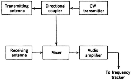
Figure 10.8 Block diagram of transmitter-receiver of CW Doppler radar.
Frequency Modulation–Continuous Wave Systems The frequency modulation–continuous wave (FM-CW) type of transmission combines some of the advantages of pulse and pure continuous wave systems. Therefore, this technique is used in the majority of dedicated modern Doppler radars. The problems of transmitter-receiver isolation and discrimination against nearby echoes are reduced or eliminated in such a system on a frequency basis, much as they are eliminated in pulse systems on a time basis. In an FM-CW system, the transmitter is sinusoidally frequency modulated, and the receiver is designed to use only the Doppler shift of a particular sideband (other than the zero-order side band) of the beat between the received and transmitted signals. Since the modulation index of the beat spectrum and hence the amplitude of all but the zero-order side bands decreases very rapidly with decreasing range and becomes zero at the receiver mixer terminals, high transmitter-receiver isolation and suppression of returns from nearby objects are achieved. Since the amplitudes of these side bands vary as Bessel functions, they are called Bessel side bands. FM-CW systems require a simple low-power sine-wave modulator/transmitter and hence their transmitter-receiver approaches pure continuous wave systems in simplicity. Since the power in only one of the side bands is used, the efficiency is not as great as that of continuous wave systems. It is maximized by the use of the optimum transmitted modulation index.
A problem with single-antenna FM-CW systems is that the combination of internal line length and mismatch of practical microwave components (antenna, switches, radome, etc.) will generate a leakage signal, which limits the achievable signal-to-leakage ratio. To alleviate this, a special leakage elimination filter is usually used. Another problem of a single-antenna FM-CW system is the fact that full transmitter-power feedthrough, which is determined by practical duplexer-isolation characteristics, is continuously applied to the receiver, regardless of the isolation obtained by the sideband processing. However, in 1996. both of these problems were overcome in FM-CW Doppler radars and single-antenna configurations were used widely.
FM-CW Doppler radars, as well as pulse modulated radars, are subject to altitude hole problems because of the relationship between modulation frequency and echo delay. These altitude holes can be eliminated by continuously changing the modulation frequency or by using different modulation frequencies over different preset altitude ranges.
The important parameters that affect the performance of FM-CW systems are (1) the order of the side band, (2) the modulation frequency, and (3) the modulation index. The order of the sideband (i.e., whether the first, J1, or a higher-order Bessel side band is used) determines low-altitude performance, effective transmitter-receiver isolation (signal-to-leakage ratio), and, to a less extent, the signal efficiency (signal-to-noise ratio) of the system. The first-order J1 system inherently permits operation down to zero-feet altitude and exhibits a flat (constant) signal-to-noise ratio versus altitude characteristic for the lower altitude region of operation [16, 37]. However, it has the lowest effective transmitter-receiver isolation and, hence, the lowest achievable signal-to-leakage ratio. The second- and third-order J2 and J3 systems have a greatly improved transmitter-receiver isolation performance (in view of the slope of the Bessel functions near zero) and still permit reasonably good low-altitude performance. In general, then, the higher the order of sideband used, the better the isolation but the worse the low-altitude performance. In 1996, the first-order (J1) Bessel side band was used in most Doppler radars designed for helicopters to take advantage of its relatively flat S/N characteristic at low altitudes. This approach minimizes the occurrences of unwanted returns from vibrating structures near the Doppler radar antenna while retaining adequate S/N for returns from terrain below the aircraft.
The choice of modulation frequency affects the location of the first altitude hole, transmitter-receiver isolation, and low-altitude signal performance. The use of a very low modulation frequency can cause the first altitude hole to appear above the maximum altitude of operation, thus avoiding the existence of any altitude holes over the range of interest. However, unless a low-order sideband is used at the same time, low-altitude performance is limited. A high-modulation frequency (the modulation wavelength being much smaller than the maximum altitude of operation) results in many altitude holes over the altitude range but in a much higher signal-to-noise ratio at the lower altitudes (though a somewhat lower signal-to-leakage ratio). In 1996, a relatively low modulation frequency, 25 to 30 kHz, was used in most Doppler radars designed for helicopters.
A high-modulation frequency, when used in conjunction with a homodyne (zero-frequency IF) receiver, inherently results in an intermediate frequency of sufficiently high value from a viewpoint of detector noise temperature. However, since the received Doppler spectrum is “folded” about zero frequency, the homodyne approach does not provide information on sense of velocity as required in helicopters or vertical takeoff and landing aircraft, unless additional (e.g., quadrature) circuitry is added (see Figure 10.9).
The choice of transmitted modulation index affects low-altitude performance, transmitter-receiver isolation, and the signal-to-noise ratio. Therefore, the modulation index is generally selected so as to be compatible with the order of the sideband and the modulation frequency that have been selected, primarily from the viewpoint of maximizing received power. A mathematical indication of this behavior can be obtained from the expressions for the received modulation index M and the radar-range equation modulation–efficiency factor E of an FM-CW Doppler radar. These are

Figure 10.9 Block diagram of transmitter-receiver of FM-CW Doppler radar for helicopters.

and
where
For high-modulation frequency FM-CW systems, it is necessary to average Equation 10.19 over one-half cycle of the argument in Equation 10.18. The maximum efficiency is obtained for the value of m, which makes this average a maximum. An approximate expression for this optimum value of m for the nth sideband is [20]:
The block diagram of a FM-CW Doppler radar for use in helicopters is shown in Figure 10.9. A directional coupler diverts a small amount of transmitter power to a power divider whose outputs are two signals in phase quadrature. These outputs serve as the reference or local oscillator (LO) for the two balanced mixers. The RF energy backscattered from the ground and received by the single antenna is directed via the duplexer to a power divider that generates two outputs of opposite phase which are then mixed with the two LO outputs in the two balanced mixers. The outputs of the two balanced mixers have now been translated to zero frequency and the Doppler frequency–shifted spectra of the sidebands below the carrier now appear as images to the true signals on the sidebands above the carrier. The two mixer outputs, which are in phase quadrature, are phase shifted an additional 90 degrees relative to each other and then summed, resulting in phase cancellation of the unwanted image signals while retaining the wanted signal. This approach preserves the sense of the Doppler frequency shift, since the latter can change sign during hover and backward flight of helicopters. The resultant signal contains the desired frequency spectrum above (positive shift) or below (negative shift) of each one of the modulation (Bessel) sidebands. The desired sideband is selected by filtering out all other sidebands. Single transmit/receive antennas tend to have high transmitter-to-receiver leakage resulting in a large unshifted signal at base band and at each of the sidebands. This leakage is removed in a filter that is centered at the desired sideband frequency. During low speed and hover operation, however, the true signal spectrum will have a very small frequency shift and will therefore occur close to the unwanted leakage signal. The filter that removes the leakage must therefore be very narrow (1 to 2 Hz) to avoid affecting the true signal spectrum. The output to the frequency tracker is thus the Doppler frequency-shifted spectrum offset from zero frequency by a multiple of the modulation frequency, which is typically the first (J1).
Frequency Trackers The function of the frequency tracker is to determine the centroid of power (mean frequency) of the noise like Doppler spectrum obtained from the ground echo (Figure 10.6). Practically all modern Doppler radars use some form of closed loop frequency discriminator as the frequency-tracking device. The Doppler signal is fed to one or more mixers, which mix it with a signal from a variable-frequency oscillator (tracking oscillator) and feed the output to the device that performs the discriminator function. The output from the latter is fed to an integrator and used to control the frequency of the tracking oscillator, which, in turn, can then provide the frequency-tracker output signal (Figure 10.10). During acquisition, frequency trackers usually use a sweeping operation by changing the tracking oscillator frequency linearly over the entire Doppler band of interest.
Two Doppler frequency-tracker configurations that have been used are shown in Figure 10.11. The one shown in Figure 10.11a is called the two-filter tracker. Actually, a single filter is used, but the Doppler spectrum is mixed with a tracking oscillator signal, which is square-wave frequency modulated over the extent of the spectrum width. The mixer output is fed to a low-pass filter, which therefore looks successively at the upper and lower halves of the spectrum. The filter output is phase detected against the frequency-modulated oscillator signal. The phase-detector output is then fed to the integrator and, having sense of direction, will drive the tracking oscillator until its output frequencies just straddle the center of power of the Doppler spectrum. The average frequency of the tracking oscillator output is thus the frequency that corresponds to the center frequency of the spectrum, which, in turn, is proportional to the desired velocity. This type of frequency tracker implementation normally does not provide sense of velocity direction through zero velocity, but it is simpler to mechanize and hence was used in Doppler radars for fixed-wing applications where negative velocities do not occur.
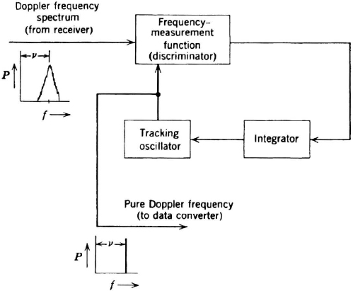
Figure 10.10 Block diagram of basic Doppler frequency tracker.

Figure 10.11 Typical Doppler frequency tracker configurations.
The frequency tracker shown in Figure 10.11b is called the sine-cosine tracker. Here the input spectrum is mixed simultaneously with the tracking-oscillator signal and its quadrature signal. The mixer outputs, which are actually the folded Doppler spectra at zero frequency, are fed through low-pass filters in two separate channels (sine and cosine) and then again phase shifted by 90°. The latter 90° phase shift may be obtained by placing a low-pass and a high-pass filter in the sine and cosine channels, respectively. The signals from the two channels are then multiplied; the multiplier output is integrated and drives the tracking oscillator, thus closing the loop. By virtue of the two quadrature channels, sense of direction for the tracking-oscillator drive is maintained. When the loop is nulled, the tracking oscillator frequency represents the average frequency of the input Doppler spectrum. Typically, the input spectrum is offset from an intermediate frequency so that sense of velocity direction is obtained from the output. The sine-cosine frequency tracker is in widespread use in modern Doppler radars and particularly in those designed for helicopters where negative velocities occur.
10.1.3 Signal Characteristics
General Criteria The performance of a Doppler radar is generally expressed by the Doppler signal-to-noise ratio (S/N) that is available at the input to the frequency tracker. The lowest S/N generally occurs at maximum altitude, speed and pitch and roll, and over terrain with the lowest radar backscattering characteristics. The performance of a Doppler radar is also affected by the sensitivity of the frequency tracker, that is, the minimum S/N at which the tracker will operate properly.
Doppler Signal-to-Noise Ratio (S/N) The Doppler S/N is a function of the following variables:
- The range to the terrain with respect to the beam of interest
- The velocity with respect to the beam of interest
- The RF backscattering properties of the terrain
- The attenuation (absorption) and backscattering properties of the atmosphere
- Radar parameters such as wavelength, receiver noise figure, transmitted power, antenna gain, beam-looking angle, transmitter and receiver path losses, and transmitter-receiver leakage noise
- The efficiency of the type of transmission (modulation) used
By modifying the basic radar-range equation [1], the Doppler signal-to-noise ratio per beam (using the same type of antenna for transmission and reception) for a coherent system in which each beam is demodulated separately is given by

| (S/N)d | is the Doppler signal-to-noise ratio (the ratio of the total Doppler signal power to the noise power, in the bandwidth of interest Bd) |
| Pt | is the average transmitted power |
| G0 | is the one-way maximum antenna gain relative to an isotropic radiator |
| λ | is the wavelength of transmission |
| E | is an efficiency factor (including the spectral modulation efficiency in pulse and FM-CW systems, gating improvements, gating losses, and noise foldover losses) |
| Lr | are losses in the radar transmitter and receiver paths, such as the wave-guide plumbing, duplexer, radome and other radio-frequency components |
| La | is the attenuation in the atmosphere |
| w | is an antenna pattern factor (normally between 0.5 and 0.67) |
| σ0 | is a scattering coefficient or backscattering cross section per unit area of the scattering surface |
| ψ | is the incidence angle of the center of the beam with respect to a normal to the surface |
| R | is the range to the scattering surface |
| NF | is the noise figure of the receiver |
| K | is the Boltzmann's constant, 1.38 × 10⁻²³ joule per Kelvin |
| Bd | is the bandwidth of interest, usually the −3-dB bandwidth of the Doppler spectrum and is proportional to velocity along the beam |
| Ki | is the effective transmitter-receiver isolation coefficient |
| (N/S)t | is the ratio of transmitter generated noise to the transmitter power |
| T | is the absolute temperature, normally taken as 290° Kelvin |
In most well-designed systems, Ki is so small that the term PtKi(N/S)t becomes negligible. Isolation is obtained by different means in different systems, such as by separate antennas in CW systems, by time separation in pulse systems, and by frequency separation (and possibly also antenna separation) in FM-CW systems. If this term is indeed negligible, Equation 10.21 becomes

Because the scattering surface fills the entire radar beam in a Doppler navigation radar, the signal-versus-range dependence in the radar range equation is the basic inverse-square law (l/R2) as given by Equation 10.22. However, for certain FM-CW and incoherent-pulse systems, the signal-versus-range dependence can vary considerably from the inverse-square law.
In FM-CW systems, E is a function of ![]() [see Equations 10.18–10.20 for the definition of
[see Equations 10.18–10.20 for the definition of ![]() ]. In low-rate frequency modulation systems (modulation wavelength of the same order as the altitude of operation, E =
]. In low-rate frequency modulation systems (modulation wavelength of the same order as the altitude of operation, E = ![]() . In these systems, since M varies with propagation delay (and hence range) and with modulation frequency and since the Bessel functions of different orders have greatly different shapes, the signal-versus-altitude dependence in specific altitude regions can vary markedly from the basic inverse-square law of Equation 10.22. In contrast, in high-rate frequency modulation systems (modulation wavelength much smaller than maximum altitude of operation),
. In these systems, since M varies with propagation delay (and hence range) and with modulation frequency and since the Bessel functions of different orders have greatly different shapes, the signal-versus-altitude dependence in specific altitude regions can vary markedly from the basic inverse-square law of Equation 10.22. In contrast, in high-rate frequency modulation systems (modulation wavelength much smaller than maximum altitude of operation), ![]() must be averaged over one-half cycle of the argument of Equation 10.18 [20]. Typical values of E for these systems range from −6.4 dB for J1 systems to − 11.1 dB for J4 systems. The average signal-versus-altitude dependence of these systems follows the inverse-square law of Equation 10.22.
must be averaged over one-half cycle of the argument of Equation 10.18 [20]. Typical values of E for these systems range from −6.4 dB for J1 systems to − 11.1 dB for J4 systems. The average signal-versus-altitude dependence of these systems follows the inverse-square law of Equation 10.22.
Terrain-Scattering Coefficient It is seen from Equation 10.22 that an important factor in determining the Doppler signal-to-noise ratio is σ0, which is the parameter of nature that determines the amount of power backscattered by the surface to the Doppler radar receiver. The σ0 factor is defined as the backscattering cross section per unit area (at the target surface), normal to the direction of propagation, intercepting that amount of power which, when scattered isotropically, would produce an echo equal in power to that actually observed per unit area of the target surface. Figure 10.12 shows curves of σ0 versus ψ angle for a radar system operating in the frequency band currently assigned to Doppler radar, namely 13.250 to 13.400 GHz. Included in Figure 10.12 are curves for various types of terrain including land and water. It is seen from the curves in Figure 10.12 that for normal wooded-land terrain σ0 is nearly constant with beam incidence angle ψ and that it has a value of −7.5 dB for the incidence angles ψ of interest (10° to 30°). However, for water surfaces, σ0 decreases radically as ψ increases and assumes different values for different conditions of sea state or water roughness. The sea-state scale shown in Figure 10.12 was developed by the United States Army to specify σ0 for their helicopter Doppler radar development programs and is typical of curves used by other development agencies. For the typical Doppler-radar incidence angles ψ of 10° to 30°, σ0 is considerably smaller for most sea states than for land and decreases markedly for the smoother sea states. Therefore, a conservative Doppler-radar design must be based on a σ0 for the smoothest sea state over which the aircraft is expected to navigate by means of the Doppler radar. (It is known, however, that very smooth sea states are relatively rare.) For physically roll-and-pitch-stabilized antenna systems, the value of ψ remains essentially constant and equal to the chosen design value. For fixed-antenna systems, a conservative design must be based on σ0 and range R for the largest ψ-angle that would be expected for the largest combination of pitch and roll angles of the aircraft.

Figure 10.12 Radar backscattering coefficient versus incidence angle for different terrains at Ke-band.
Bandwidth, Antenna Gain, and Losses The bandwidth Bd in Equation 10.22 is the effective bandwidth of the Doppler frequency tracker. In most systems, this is selected to be the −3-dB Doppler spectrum width. From Equation 10.13 we have, for a coherent or post-tracker Janus system, Bd = Δv = (2V/λ)Δγ sin γ, where γ is the angle between the velocity vector and the angle of radiation, and Δγ is the −3-dB two-way beam width in the γ-direction. (When the antenna beam pattern has a predominantly Gaussian shape in the region of interest, as is typical for Doppler radar antenna beams in the γ-direction, the two-way beamwidth is 0.707 of the one-way beamwidth.) Thus, the Doppler signal-to-noise ratio is inversely proportional to the speed of the vehicle. In view of this, the design of a Doppler radar as regards signal performance must be based on the maximum expected vehicle velocity components along each beam. The product G0λ2 in Equation 10.22 is directly proportional to antenna area A from the basic expression for antenna gain. Specifically, for an antenna of 55% efficiency, G0λ2 = 7A. Thus, the Doppler signal-to-noise ratio is proportional to antenna area. (This is strictly true only for a radar using transmitting and receiving antennas having the same area.)
For the transmission wavelength normally used for Doppler radar (2.2 cm) and considering the relatively short ranges to the ground (when compared to those of forward looking search radars), the attenuation La due to the atmosphere and to typical rain rates are found to be very small.
From Equation 10.22, the noise figure of the receiver NF is an important parameter; it has therefore been an objective in Doppler-radar design to achieve the lowest possible receiver-noise figure. Similarly, the radio frequency losses Lr of the microwave circuitry must be kept as low as possible.
Frequency-Tracker Sensitivity In addition to the available signal-to-noise ratio, the other parameter that determines the signal performance of a Doppler radar is the sensitivity of the frequency tracker. This is usually expressed by two quantities, namely, the acquisition sensitivity (i.e., the Doppler signal-to-noise ratio at which the Doppler signal can be acquired and tracking begins) and the tracking or dropout sensitivity (i.e., the Doppler signal-to-noise ratio at which tracking stops, and the system may be placed into a memory mode). The acquisition sensitivity depends on the Doppler signal-to-noise ratio required to achieve the specified accuracy and to avoid locking on to extraneous noise signals such as second harmonic spectra. In typical Doppler radars, the acquisition sensitivity is set at a Doppler signal-to-noise ratio of approximately 5 dB. A signal-to-noise detector is normally used to place the radar automatically into the tracking mode when this Doppler signal-to-noise ratio is present. This circuit continuously samples the received signal level and the system noise level (or its equivalent) and measures their ratio so as to determine whether a sufficiently high signal-to-noise ratio is present for acquisition and tracking. The tracking, or dropout, sensitivity is the Doppler signal-to-noise ratio level at which the signal-to-noise detector is set to cause the frequency tracker to stop tracking. In typical Doppler radars, the frequency-tracker dropout sensitivity is approximately 3 dB.
Full Doppler radar accuracy (particularly the Doppler fluctuation error) is frequently not obtained unless the Doppler signal-to-noise ratio is between 7 and 10 dB. Therefore, systems utilizing Doppler velocity data only for critical or sensitive functions (versus integrated velocity for navigation) should require minimum Doppler signal-to-noise ratios of near 10 dB.
10.1.4 Doppler Radar Errors
Classification of Errors Doppler radar velocity errors can be classified as either random (varying with time) or systematic (independent of time). Random errors are those errors that vary during a flight or flight leg. Systematic errors are those that are constant, although perhaps unknown, for the duration of the flight. Known systematic errors can be calibrated out, either before the start of a mission, after equipment installation in the aircraft, or even at the factory. All uncompensated systematic errors must be included in an error analysis. There are two types of random errors: those with relatively long correlation times and the Doppler-fluctuation noise that has a correlation time τc (at the output of the frequency tracker) on the order of 0.1 sec. Both of these are typically assumed to be exponentially autocorrelated. Since 15 minutes would be the least desirable correlation time for a velocity error in a Doppler radar used in a Doppler-inertial system—because of the effects of the Schuler period (Section 7.6.3)—it has been of special interest to keep Doppler velocity errors having correlation times near 15 minutes as low as possible. Another classification of errors is that of percentage-of-speed or scale-factor errors, and errors independent of speed or speed-offset errors. Most errors are scale-factor types. In this section, each of these various errors is treated separately, followed by a discussion of the total Doppler radar velocity error and the Doppler-navigation system errors. The coordinate system that is most suitable for describing the errors of a Doppler radar with a fixed antenna is (H′, D′, V′), as described previously (Equations 10.4 to 10.6).
Doppler-Fluctuation Error The Doppler fluctuation error ef is due to the noiselike nature of the Doppler signal spectrum, which, in turn, is caused by the backscattering properties of terrain. The standard deviation of the basic Doppler velocity fluctuation error per beam of a coherent system, assuming a perfect frequency tracker, can be expressed by [3]:

where
If the beam has a Gaussian shape, which is typical for Doppler radar beams in the region of interest, the 2-sigma two-way beamwidth is equal to 1/1.18 times the −3-dB beamwidth). In Equation 10.23, τv represents the Doppler correlation time 2/Δv″ (at the input to the frequency tracker; in contrast to the correlation time tc at the output of the frequency tracker, discussed previously). K1 is a constant combining the various radar parameters and constants in the expression.
From the standpoint of navigation between two points (separated by many antenna lengths and many frequency tracker time constants), T is the total time flown. It is seen from this equation that V and T occur only as a product and hence can be replaced by the distance flown D:

Equation 10.24 indicates that the basic Doppler velocity fluctuation error is inversely proportional to the square root of the distance traveled. A physical explanation of this can be obtained by realizing that it is the total number of independent scatterers seen by the Doppler radar beam that determines the amount of smoothing afforded and hence the final velocity fluctuation error.
Equations 10.23 and 10.24 express the Doppler velocity fluctuation error under ideal or error-free frequency measurement conditions. The performance of a practical system will differ from an ideal one by some factor N, which has been called the performance factor:

where N is a factor that relates measured values to theory. For practical equipment, N has a value somewhere between 1 and 2. The all-digital frequency tracking circuits used in 1996 resulted in N being nearly equal to 1. A typical Doppler radar operating at 13.3 GHz and with a beamwidth of 6° has a fluctuation error of 0.051% after 10 mi and 0.016% after 100 mi of travel. Thus, the fluctuation error is negligible after only a few miles of travel when compared to other instrumentation errors of the system. Doppler radar velocity accuracy specifications are usually cited for a condition of “after 10 mi of flight.”
Equations 10.23 and 10.24 give the fluctuation error per beam, assuming single beam tracking. Modern systems measure each of the four beams sequentially and then combine the four beam velocities to arrive at V′H, V′D and V′V. Each beam is tracked for 25% of the time, which increases ![]() by (4)1/2, but four beams are combined and thus
by (4)1/2, but four beams are combined and thus ![]() decreases by (4)l//2. Equation 10.24 thus applies to
decreases by (4)l//2. Equation 10.24 thus applies to ![]() ,
, ![]() , and
, and ![]() as well, except that Δγ″ is replaced by ΔγH, ΔγD, and ΔγV, and γ by γH, γD, and γV:
as well, except that Δγ″ is replaced by ΔγH, ΔγD, and ΔγV, and γ by γH, γD, and γV:


When quasi-instantaneous short-term velocity information is considered, the smoothing time T in Equation 10.23 represents the integration time constant of the Doppler radar frequency tracker. Clearly, the longer the time constant, the lower will be the fluctuation error. However, the shorter the time constant, the better will be the system response to velocity changes (accelerations). In typical aircraft systems, this time constant is approximately 0.1 sec.
For certain applications, notably in Doppler-inertial systems, it is frequently of interest to find the power spectral density per unit of speed of the Doppler-fluctuation error, called P0. The fluctuation component of the velocity error at the output of the frequency tracker is assumed to be white noise over the frequency range of interest in Doppler-inertial system analysis. This is based on the fact that the Doppler signal received in the frequency tracker has the properties of band-limited noise and, to a first approximation, this spectrum has a Gaussian shape with a half-width proportional to speed. This spectrum width determines the standard deviation of the fluctuation. The result of this is a velocity error spectrum with power spectral density at zero frequency which is proportional to speed; that is, the power density is equal to P0V. This noise is then filtered by the frequency tracker and the radar velocity readout circuitry, which act as low-pass filters. The relationship of P0 to the standard deviation of the relative Doppler fluctuation error ![]() is expressed by
is expressed by

where P0 is the velocity error angular spectral density per knot of speed (the statistical “power” value of the error source has the dimension of knots2 and P0 is in units of knots2 per (radian/second) per knot, which is in units of distance, namely, knot-seconds. Typical values of P0 for operational systems in 1996 were between 0.003 and 0.005 knots2 per (radian/second) per knot for V′H and V′D and approximately 2.5 times smaller for V′V.
Errors in Beam Direction As seen from Equations 10.4 to 10.6, the nominal beam angle γ0 must be accurately known and maintained in order to permit accurate measurement of velocity. The basic fractional velocity error ![]() for an error in beam direction δγ is
for an error in beam direction δγ is
An error in beam direction of one minue of arc and a nominal γ0-angle of 70° yields an error of 0.08% of ground speed. (When four beams are used for velocity determination, the total effect of the random error in direction in each of the four beams is reduced by the square root of four.) Beam direction errors resulting from radome refraction effects, and temperature effects in certain antennas (notably linear and planar waveguide arrays) will contribute to ![]() . This scale-factor error is primarily systematic and, in most cases, can be largely removed by some form of ground or flight calibration procedure. Because of the smaller effective γ-angle, the equivalent error in vertical velocity is an order of magnitude smaller than that in ground speed.
. This scale-factor error is primarily systematic and, in most cases, can be largely removed by some form of ground or flight calibration procedure. Because of the smaller effective γ-angle, the equivalent error in vertical velocity is an order of magnitude smaller than that in ground speed.
The temperature error in slotted array antennas is proportional to the deviation from the calibration temperature and the linear coefficient of expansion of the antenna material. In typical systems, this error is less than 0.05% for the horizontal velocity component and approximately one-tenth of this for the vertical velocity component.
Error in Transmission Frequency As seen from Equation 10.4 to 10.6, the knowledge and maintenance of the transmission frequency f (or wavelength λ) directly affects the value of the measured Doppler frequency and hence the measured velocity accuracy. The long-term frequency stability of modern solid-state microwave sources is typically in the range of 10−4 to 10−6, resulting in a negligible error. Moreover, linear and planar slotted array antennas for Janus systems can be designed so as to make the Doppler calibration constant completely independent of transmission frequency, that is, dependent only upon slot spacing.
Error in Frequency Measurement (Frequency Tracker Bias) This error is a function of frequency tracker design and is usually caused by unbalance in the frequency tracker discriminator. Also, a nonuniform noise power density in the frequency tracker bandwidth will cause a bias error in the frequency measurement whose value is generally a function of Doppler signal-to-noise ratio. In 1996, frequency trackers use digital signal processing techniques for which this error is typically less than 0.05 knots at 6 dB or higher S/N.
Altitude-Hole Error Certain pulse and FM-CW systems exhibit a residual error due to spectrum-weighting effects in the altitude-hole regions due to the effect of the modulation periods, even if some form of modulation wobbling is used. Typical values for the residual altitude hole error using modulation wobbling are less than 0.02%.
Land-Terrain Error Over land terrain a small error results from (1) range-difference effects over the beam width, (2) the nonlinear function of converting ray angles within the beam width to Doppler frequencies (see Equation 10.3), and (3) the small change in scattering coefficient with looking angle over the beam width (Figure 10.12). The first two effects are very small and may be eliminated by flight calibration. The third effect is exactly the same type as the overwater calibration shift error described in the next paragraph. Because of the very small change in scattering coefficient over the beam width for typical land terrain (Figure 10.12), this error is normally quite small, unless a very small antenna with a large beamwidth is used. A 6 × 12 in. antenna would have an error of about 0.1%.
Overwater Errors The three different types of overwater errors of Doppler radars are (1) the calibration-shift error, (2) the sea-current error, and (3) the surface wind induced water-motion error.
The overwater calibration-shift error (or sea bias) results from the change in the scattering coefficient σ0 versus incidence angle ψ over the antenna beam width, as it relates to the direction of changing Doppler frequencies, that is, normal to the isodops. The phenomenon is evident from Figure 10.12 which shows a plot of σ0 versus ψ for various sea states. A Doppler radar with a nominal ψ-angle of 20° and a beam width of 5°, covering a ψ-angle range of 17.5° to 22.5°, has a significant change in scattering coefficient σ0 over water. The slope m in the σ0 curve will cause the Doppler spectrum to be weighted in the direction of lower Doppler frequencies and will therefore cause the frequency tracker to read out too low a velocity. This is illustrated in Figure 10.13, which shows plots of typical (artificially smoothed) Doppler power spectra over land and water. The mean of the Doppler spectrum obtained over land (i.e., frequency vl), represents the correct frequency for the speed of the vehicle. The lower power spectrum is the Doppler spectrum over water for the same vehicle speed, having a mean frequency vw. The difference between vl and vw is the overwater calibration shift error or sea bias. For an antenna pattern having a Gaussian shape and for a linear function of the logarithm of σ0 (in decibels) versus ψ within the beamwidth, which is a good approximation, as seen from Figure 10.12, the resultant overwater spectrum has a Gaussian shape like the overland spectrum but with its centroid of power shifted by vl − vw (Figure 10.13). Figure 10.13 shows that at any nominal ψ0 the slope of σ0 versus ψ changes for different sea states, and, since the overwater calibration shift error is a function of this slope, the error has different values for different sea states.

Figure 10.13 Doppler spectra (smoothed) over land and water.
An exact determination of the calibration shift error is obtained by integration of the elemental powers returned by the antenna beams as a function of Doppler frequency (along the isodops) and as a function of the scattering coefficient and incidence angles for different terrains and sea states (Figure 10.12). For typical Doppler systems (for level flight), an excellent approximation of the uncompensated calibration shift error in percent is given by
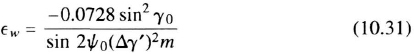
where
| ψ0 | is the nominal (central) beam incidence angle (Figure 10.4) |
| Δγ′ | is the 3-dB one-way γ-beam width, in degrees |
| m | is the slope of the γ0 versus ψ curve at the ψ0 angle, in decibels per degree |
| γ0 | is the angle between the longitudinal axis of the aircraft and the beam centroid (Figure 10.3) |
For typical Doppler radar parameters, the uncompensated error given by Equation 10.31 is approximately
Equations 10.31 and 10.32 are also valid over land terrain but are typically negligible because m is generally small. Over water, however, if no compensation techniques were used, ![]() could take on peak values anywhere between 1% and 5% over an extreme spread of sea states, depending on the radar parameters used. Note also the strong dependence upon Δγ′ and thus on antenna size.
could take on peak values anywhere between 1% and 5% over an extreme spread of sea states, depending on the radar parameters used. Note also the strong dependence upon Δγ′ and thus on antenna size.
Several techniques have been developed to compensate for the overwater calibration shift or sea bias error. Early Doppler radars often employed a manual land-sea switch operated by the flight crew. When the switch is in the sea position, an overwater calibration shift correction is added to the Doppler radar velocity output corresponding to the most frequently occurring sea state expected on the missions flown. The residual error is the difference between the actual sea state and the one used for calibration. Based on a Gaussian distribution of the probability of sea-state occurrence and a properly chosen land-sea switch setting, the residual overwater calibration-shift error for this land-sea switch technique is near 0.3% to 0.6% (1-sigma).
A fully automatic technique for sea bias compensation used in early Doppler radars was lobe switching [19]. In this technique, each antenna beam is oscillated periodically by a small amount in the γ-direction at a low rate (e.g., 20 Hz). If the oscillations are square wave, the return signal consists of two Doppler spectra existing alternately in time at the switching rate. The frequency tracker (which bears some similarity to the two-filter tracker discussed in Section 10.1.2) effectively places a narrow filter at the point where the two spectra have equal power or crossover and reads out the corresponding frequency as the aircraft's velocity. The crossover point at a particular aircraft speed is the same for both land and water, since the returned energy for the two spectra were derived from the same group of scatterers and at the same incidence angle. A similar technique using simultaneous lobing by means of a “monopulse” type antenna achieves essentially the same effect [34].
The lobe-switching and simultaneous lobing techniques achieve a large reduction in the overwater (and overland) calibration-shift errors but can cause a significant increase in cost and complexity. For these reasons they are being replaced by newer techniques, such as beam shaping, wherein the calibration shift is reduced by the use of a special beam geometry. In this approach the beam geometry is shaped to cause the centroid of the beam to remain at the same γ-angle even when the slope m of σ0 has changed. In 1996, antenna design and fabrication techniques provided considerable flexibility in shaping the beam to the desired geometry. In one technique, the beam is generated as the product of a function of γ-angle, f(γ), and a function of ψ-angle, f(ψ). The received signal is the product of f(γ), f(ψ), and σ0(ψ). For small variations in ψ, σ0 can be replaced by (m × ψ). A change in m causes [f(ψ) × m × ψ] to change but not f(γ). Thus, the resultant spectrum shape is that of f(γ), since [f(ψ) × m × ψ] multiplies all elements of f(γ) equally. The overwater calibration shift in the forward or H′ direction is reduced to the extent that the beam shape approximates [f(γ) × f(ψ);]. The calibration shifts in the D′ and V′ directions are not compensated by this technique but are generally small, since V′D and V′v are small compared to V′H. In 1996, a residual overwater shift bias of 0.1% to 0.2% was achieved with this technique. As an aircraft flies over areas of changing sea state, the residual error will appear as a slowly varying random error of 0.05% to 0.1%.
Sea-current and tidal effects result in errors, because the Doppler radar measures velocity relative to the moving sea surface, giving rise to a navigation error relative to the Earth. Fortunately, the speed of sea currents is generally very low. According to available information, general random sea currents rarely exceed a speed of 0.4 knots. Also, since these random currents have random directions, their effects tend to average out for flights of any appreciable distance. Major currents such as the Gulf Stream have a maximum surface speed of less than 3 knots. Where necessary, manual compensation for flight over major sea currents can be made in the navigation computer in flight or before the start of a flight. The sea-current error is a bias, speed-offset error.
In some special applications, such as the dropping of sonobuoys in antisubmarine warfare, the velocity of the aircraft with respect to the sea is actually the desired quantity, and no sea-current correction need be made.
The surface-wind water-motion error is caused by wind-blown water particles at and above the surface of the sea. Since these surface water droplets are a portion of the scattering surface seen by the Doppler radar beams, their motion results in an error in the velocity measurement. Theoretical analysis and actual measurement of this error have revealed that the error is [24]
where ![]() is the surface-wind, water-motion error in knots and W is the surface-wind speed.
is the surface-wind, water-motion error in knots and W is the surface-wind speed.
It has been found experimentally [23] that this effect is not observable at wind speeds of less than 2 knots. Experiments have also shown that the angular difference between the mean spray direction and the wind direction is generally below 30° [23]. For automatic correction of this error by means of surface-wind data, it is reasonable to assume that the direction of the error is in the direction of the wind. The surface-wind water-motion error is a bias speed-offset error. Since the direction of surface winds varies over any appreciable area, the surface-wind, water-motion error will be reduced by averaging. It is of interest to note that the water's wave motion as such does not produce any Doppler radar error, since the water particles are not actually moved forward in the wave action but undergo a periodic up and down movement.
Maneuver-Induced Errors Aircraft maneuvers, such as acceleration and turns, cause the components of velocity along the beams to change. The frequency trackers must follow these changing frequencies. To reduce short-term fluctuation noise, a smoothing time of about 0.1 sec is usually incorporated into the frequency tracker. As a result, a velocity lag exists in the presence of acceleration. If the tracker dynamics are first order, this velocity error is approximately equal to half the acceleration times the smoothing time. Fortunately, such errors are transient and can be further reduced by appropriate frequency-tracker instrumentation, such as the use of a double integrator in the tracker loop. In fixed-antenna systems, aircraft pitch and roll rates can give rise to changes of Doppler frequency like those produced by aircraft acceleration and will cause equivalent lag errors if the tracker dynamics are not capable of following them. Therefore, fixed-antenna systems are more demanding on tracker dynamics than physically pitch-and-roll-stabilized antenna systems (Section 10.1.2).
Error of Attitude Stabilization or Conversion from Vehicle to Ground Coordinates The basic Doppler velocity information is obtained in antenna coordinates, which, in the case of fixed antennas, are the same as aircraft coordinates. Velocity is required in ground coordinates for purposes of navigation and is therefore transformed through the pitch and roll of the vehicle in a stabilization computer, which receives the pitch-and-roll information from the vertical reference (Chapter 9). The resulting error then depends on the error in the vertical reference and the stabilization computer, as well as on the values of pitch, roll, and drift and on beam geometry. The error due to roll is relatively small as long as the drift angle is small. Furthermore, roll angles tend to average out over reasonable flight lengths; pitch angles generally do not, because of angle-of-attack changes due to aerodynamic loading and prolonged periods of climb and descent.
Using partial differentiation techniques in connection with Equations 10.9–10.11, which inherently assumes that the errors in pitch and roll are small, the following expressions can be derived for the errors in the three orthogonal velocity components in ground coordinates resulting from errors in pitch and roll in either a pitch-and-roll-stabilized system or a fixed-antenna system that is compensated for pitch and roll:

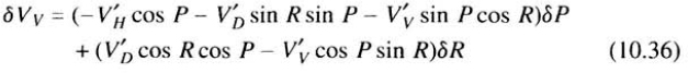
| δVH, δVD, and δVV | are absolute errors in the along-heading, cross-heading, and vertical-velocity components in Earth coordinates |
| are along heading, cross-heading, and vertical-velocity components in aircraft coordinates | |
| δP | is the pitch-angle error |
| δR | is the roll-angle error |
Equations 10.34 through 10.36 can be further simplified by expressing the errors as a function of ground velocity components (VH, VD, VV), namely,
For a pitch-and-roll-compensated system, the approximate errors ΔVg in ground speed and Δδ in drift angle δ are

Calibration Error In 1996, the primary errors in the calibration constants of Doppler radars result from errors in the central antenna beam looking angles. The effect of errors in these angles on the velocity output can be obtained by differentiating Equations 10.4, 10.5, and 10.6 with respect to α0 and θ0. The departure of each beam angle from its nominal value can be measured by flight test or on an antenna range. Values below 0.05% are typical for this error.
Installation Error When installed in the aircraft, the antenna must be accurately aligned with either the longitudinal axis of the aircraft or the reference axis of the heading reference. In fixed-antenna systems, an azimuthal error in antenna installation will contribute to both of the horizontal-velocity component scale-factor errors of the system. In track-stabilized systems, an azimuthal antenna misalignment results directly in a bias error in drift angle. Antenna-installation errors about the pitch-and-roll axis have the same effect as the attitude errors discussed previously. Generally, pitch-and-roll installation errors have a significant impact only on vertical velocity accuracy.
Error in Data Conversion and Readout In 1996, electronic frequency-to-digital conversion devices exhibit errors between 0.01% and 0.05%. For use with digital navigation computers, Doppler frequency velocity data are converted into binary digital form with very small errors. In such a digital system, the error is a function of the time-base inaccuracy and of the number of binary bits used. Since these digital quantization errors are uniformly distributed, the standard deviation of the error is obtained by dividing the quantization error by ![]() .
.
Doppler Radar Velocity Errors There are three types of errors:
- Bias, speed-offset errors
 (expressed in knots), which cause position
  , where T is the time since the last fix. Unknown offset bias errors can be calibrated for the mean bias expected on an ensemble of flights; is the deviation of the offset bias from the calibrated value.
 - Bias scale-factor errors
 (expressed in percent), which cause velocity
  times Vi, where Vi is the velocity component V′H, V′D, or V′V, and
  is the corresponding scale-factor error. The scale factors are calibrated for the mean value expected in flight; is the deviation from the calibrated value.
 - Random velocity errors. These are generally errors assumed to have zero mean; that is, the mean is included in errors 1 or 2 above. If the random velocity errors have a mean square
 and are assumed to be exponentially autocorrelated with a correlation time Tr, which is much less than the flight time T, the distance error
  . These random errors generally consist of two types; those with relatively long correlation times, and the Doppler-fluctuation error, having a correlation time of 0.1 sec. These errors are frequently expressed as a fraction of distance traveled (or a fractional speed error) after a total smoothing distance D, such that
  . Hence, they cause a position error that is proportional to the inverse square root of D.
Since the individual error sources are statistically independent, the total velocity component errors are obtained by taking the square root of the sum of the squares (rss) of the individual errors. This rss combination of errors should then represent the average performance of many systems on many flights. The Doppler radar velocity error is normally expressed in terms of the three orthogonal velocity components σVH, σVD, and σVV. Since each of these component errors is assumed to have a normal probability distribution, the standard deviation error σ is the 68% probability error (Section 2.7).
In 1996, typical lightweight small-size Doppler radars, operating over land and after 10 nmi of travel, have standard deviation velocity errors of less than 0.25% plus 0.1 kn.
The above errors describe the Doppler velocity error for overland operation. For overwater operation, errors due to water motion and the calibration shift error (due to the larger slope of the radar backscattering coefficient versus incidence angle) must be included. In 1996, Doppler radars typically employ beam shaping to automatically compensate for the overwater calibration shift, resulting in a residual error of 0.1% to 0.2%. The residual water-motion error after compensation for the known water motion effects in the operating area is typically 0.5 knots. The resultant velocity error due to overwater operation is (0.15% + 0.5) knots 1-sigma, which must be added to the overland errors to obtain the total overwater error.
TABLE 10.1 High-performance Doppler radar velocity errors (over land)

High-performance Doppler radars have been designed that have total standard deviation errors less than half of those cited above. Most of the Doppler radars of that type included either the lobe switching [19] or simultaneous lobing [34] overwater calibration-shift compensation technique. These high-performance Doppler radars exhibited overland V′H and V′D velocity component errors as shown in Table 10.1.
For overwater operation, the residual water motion error of 0.5 kn plus the residual overwater calibration shift error of 0.035% must be added to the values in Table 10.1, resulting in a total overwater error of (0.11% + 0.5 kn) (1-sigma). The V′V component velocity error is generally two to three times smaller than the V′H and V′D components.
Doppler-Navigation System Errors Doppler velocity information is measured in aircraft coordinates and must be transformed through aircraft heading, pitch and roll in order to generate the desired navigation information. The effects of pitch-and-roll errors on horizontal navigation are small and can generally be ignored. Heading errors affect horizontal velocity, and hence navigation directly. Quantitatively, a 1° error in heading represents a 1.75% cross-track position error, as given by the expression σTh(%) = 1.75σh(deg) where σTh is the percent standard deviation of the cross-track distance error due to heading error, and σh is the standard deviation of the heading error in degrees. Heading error can thus have a major effect on Doppler-navigation system accuracy. In 1996, navigation computers are digital and contribute a negligible error.
The total position error of a Doppler-navigation system is thus determined by the errors of the two major components of the system, namely, the Doppler radar and the heading reference. The position error may be determined on the basis of these errors and statistical considerations of the problem as a two-dimensional error problem (Section 2.7). The two dimensions usually chosen are the along-track and cross-track directions, frequently called range and transverse directions, respectively. This assumes, as is generally justified for Doppler-navigation systems, that the covariance matrix of the errors is diagonalized along these directions, so these errors may be considered independent. The range error σR consists of the error in Doppler along-heading velocity σH, and a very small second-order contribution of heading error. The latter is so small that it can safely be neglected. Thus, σR can be taken as equal to σH. The cross-track (transverse) error σT consists of the error in Doppler cross-heading velocity component σD and the error due to the heading reference σTh. In this dimension, the heading error is first order and generally is the dominant error. Based on measured results, the range and transverse errors exhibit roughly normal probability distributions. The resulting position error therefore exhibits a two-dimensional normal or elliptical probability distribution (Section 2.7), the two dimensions being σR and σT. The standard deviation of σT is given by the root sum square of the two individual cross-track errors: ![]() . Measured results [8, 26] have shown that σR and σT, and hence the percent position error, of Doppler-navigation systems are inversely proportional to the square root of the distance traveled. This behavior may be attributed to the effects of the smoothing of certain slowly varying errors.
. Measured results [8, 26] have shown that σR and σT, and hence the percent position error, of Doppler-navigation systems are inversely proportional to the square root of the distance traveled. This behavior may be attributed to the effects of the smoothing of certain slowly varying errors.
Flight test results of complete Doppler-navigation systems have shown 68% probability position errors of near 1 % of distance traveled. The results of an extensive flight test program on a military system [24] showed 1-sigma range (along-track) errors near 0.25% and transverse (cross-track) errors near 0.5% for 1000-mi flight lengths, which amounts to a 68% probability position error of 0.63%. These systems used gyromagnetic heading references and analog computers of that period and had no automatic overwater calibration shift compensation techniques incorporated into them. In 1996, the performance improvement of heading references (Section 9.4) and digital navigation computers made it possible to capitalize on the inherent accuracy capability of Doppler radars. Also, the various automatic overwater calibration shift compensation techniques have greatly reduced the previously largest error of the Doppler radar itself, namely, the overwater bias error. The effect of these performance improvements was verified during a flight test in a fixed-wing aircraft of a fixed-antenna FM-CW Doppler radar with beam shaping (for overwater bias correction) and an inertial quality heading reference. This test exhibited an along-track error of 0.14% (1-sigma) and a cross-track error of 0.15% (1-sigma) [7], The flight test consisted of 207 legs over land for a total distance of over 6000 nm.
In 1996, large quantities of military helicopters were outfitted with Doppler-navigation systems. In most cases, these systems used a magnetic heading reference, and their flight profiles consisted of short legs (10 to 20 nmi) between waypoints. Typical total position errors exhibited in flight tests were along-track error of 0.25% (1-sigma) and cross-track error of 1% (1-sigma) of distance traveled. The cross-track error is strongly dependent upon the accuracy with which the magnetic compass is calibrated or “swung.” In some applications the compass “swing” is performed in flight by flying over known checkpoints and measuring the position error on that leg and on that course. The cross-track component of the position error, converted into degrees, is then inserted into the navigation computer and used to correct subsequent flights at that course angle. The process can also be performed using electrical swinging (see Section 9.4.6).
10.1.5 Equipment Configurations
One of the first Doppler radar equipments developed, the AN/APN-81, which became operational in approximately 1956. weighed approximately 290 lb, radiated 50 w of average power, and consumed 1700 w. When the navigation computer was added, the total weight of the Doppler navigation system was 700 lb. Doppler systems performing the equivalent function in 1996, weighed 12 lb. including the antenna, all electronics, and a MIL-STD-1553 data bus interface (Section 15.2); they radiate 20 mw of average power and consume 20 w.
Figure 10.14 shows the AN-ASN-157 Doppler-navigation system for helicopters. The antenna is at the bottom of the unit. It uses a single four-beam fixed antenna, a Gunn diode transmitter, and an integrated receiver/antenna beam-switching module. The modulation is FM-CW, with a modulation frequency of 30 kHz. Its weight is 12 lb. Variations of that type of system use multiple modulation frequencies to overcome altitude hole effects above 15,000 ft. Another single–unit FM-CW Doppler radar is the CMC-2012, designed for helicopter operation. It has a MIL-STD-1553 data bus interface. Its horizontal velocity range is −50 to +350 knots, and this particular radar has demonstrated a three-axis hover accuracy of 0.72m/min. In 1996, Doppler-navigation systems weighing 9 lb were operational in drones providing navigation and altitude above terrain. The latter systems usually employ the FM-CW technique described in Section 10.2.4.
Considerable effort was underway in 1996 on combining Doppler radars with GPS (Section 5.5) by embedding a GPS receiver module into the Doppler radar unit and using the data from both sensors [9]. This approach combines the high accuracy of GPS (Section 5.5.10) and the continuous dead-reckoning operation of Doppler navigation. Use of the GPS data solves the initialization problem of dead-reckoning navigation systems. For low altitude operation, such as in helicopters, the Doppler radar provides continuity of navigation when GPS signals are not available or loss of tracking occurs, due to terrain, foliage masking, severe maneuvers, or jamming. Also, the Doppler radar can provide accurate velocity for aiding the GPS-tracking loops during acquisition in GPS State-3 operation. Use of the GPS data overcomes the Doppler-navigation system limitation of increasing position error with distance traveled due to heading reference and Doppler velocity errors and water motion errors. In 1995, such a Doppler/GPS navigation set was successfully flight tested by the U.S. Army [30]: and by 1996 production of it was in progress.

Figure 10.14 AN/ASN-157 Doppler radar (courtesy, GEC-Marconi Company).
10.2 RADAR ALTIMETERS
10.2.1 Functions and Applications
The basic function of the radar altimeter is to provide terrain clearance or altitude with respect to the ground level directly beneath the aircarft. The altimeter may also provide vertical rate of climb or descent and selectable low altitude warnings. In 1996, radar altimeters typically weighed 4 to 10 lb, exhibited a 1.5 ft or 2% altitude accuracy and transmitted 5-w peak pulse or 500-mw average CW power for a 5000-ft altitude capability. Altimeters built during the early 1960s weighed 15 lb or more and transmitted 100 w of peak pulse power. Performance characteristics are designed to match particular applications. High-performance low-flying military aircraft and cruise missile systems require accurate altitude tracking at vertical rates of over 2000 ft/sec while maintaining a high degree of covertness and jam immunity. Altimeters designed for terrain correlation for navigational purposes (Chapter 2) must process an extremely small ground illumination spot size at high altitudes to provide the required altitude resolution. Altitude marking radars are generally low altitude altimeters designed specifically to provide mark signals at specific altitudes for initiation of an automatic operation such as fuze triggering on submunitions or chute opening on lunar-landing systems. Radar altimeters for civil aviation are designed to support automatic landing, flare and touchdown computations (Chapter 13).
10.2.2 General Principles
Altimeters perform the basic function of any range measuring radar. A modulated signal is transmitted toward the ground. The modulation provides a time reference to which the reflected return signal can be referenced, thereby providing radar-range or time delay and therefore altitude. The ground represents an extended target, as opposed to a point target, resulting in the delay path extending from a point directly beneath the aircraft out to the edge of the antenna beam. Furthermore, the beam width of a dedicated radar altimeter antenna must be wide enough to accommodate normal roll-and-pitch angles of the aircraft, resulting in a significant variation in return delay. For example, a typical 50° beam-width antenna, at 5000-ft altitude, provides an altitude delay of 5000 to 5500 ft over flat terrain. The resulting altitude error becomes even greater, and potentially dangerous, when flying low over mountainous peaks with the wide antenna beam illuminating adjacent valleys. To provide range to the nearest return within the bounds of the antenna beam, many modern radar altimeters incorporate a leading edge range tracker servo loop. The tracker functions to position the gate in a pulse modulated radar or a filter in a frequency-modulated radar over the leading edge of the return.
Frequency Band The frequency band of 4.2 to 4.4 GHz is assigned to radar altimeters. This frequency band is high enough to result in reasonably small sized antennas to produce a 40° to 50° beam but is sufficiently low so that rain attenuation and backscatter from rain have no significant range limiting effects.
Antenna Requirements Typical installations include a pair of small microstrip antennas for the transmit and receive functions. The antennas typically provide 10-dBi gain with a 50 × 60 degree beam. A 30-in. spacing between transmit and receive antenna provides about 85-dB isolation. The antennas are spaced to provide isolation loss greater than the maximum expected ground return loss at low altitudes. At low altitude, the radar loop sensitivity is limited, as a function of altitude through a sensitivity range control (SRC) mechanization, to allow the altimeter to detect the ground return without detecting antenna leakage.
10.2.3 Pulsed Radar Altimeters
The basic pulsed radar altimeters of the early 1960s typically operated with 100-w cavity-tuned tube oscillators to provide performance to 5000 ft. These early radars evolved to 5-w solid state transmitters incorporating receiver pre-amplifiers in the 1970s and provided a high degree of reliability, low probability of intercept (LPI), small size, and high accuracy. During the 1980s, the discrete transmit/receive RF circuits were replaced with GaAs MMIC's (Microwave Monolithic Integrated Circuits). In 1996, receive/transmit functions were being accomplished with RF hybrid packages incorporating the GaAs MMIC functions. Advances in digital integration technology allowed replacement of the analog leading edge altitude tracker loops with digital altitude tracker loops. Although the basic radar altimeter functions have not changed significantly, incorporation of these technology advances resulted in vastly improved performance and reliability at a fraction of the cost and size of earlier systems.
The functional diagram of Figure 10.15 illustrates the basic operation of pulsed altimeters. The PRF generator provides the modulation wave form for the transmitter and a t0 time mark for the tracker loop. The transmit signal is derived from a stabilized oscillator, modulated, and amplified to the desired power level. The receiver low-noise amplifier (LNA) typically has a 2- to 3-dB noise figure, resulting in a sensitivity level that allows relatively low transmit power (1 to 5 w). A separate stabilized local oscillator (LO) provides down conversion to the IF for band limiting, amplification, and envelope detection. The track loop positions the range gate at the leading edge of the signal return to provide “gate overlap” energy corresponding to the leading edge threshold reference. The Class-2 servo loop, consisting of range rate-and-range integration, is designed to provide the track rate required to follow terrain elevation change rates at the velocity limits of the particular aircraft. This typically results in a closed loop bandwidth of 100 Hz to provide a 2000-ft/sec range rate capability. The integrated gate position error is added to the altitude register that repositions the gate through the altitude to time delay converter. The time delay converter is typically a high-speed counter or analog ramp generator referenced to the transmit t0 time mark. Additional functions not shown in Figure 10.15 include noise AGC to control IF gain, closed loop transmit power management control (PMC) to maintain minimum transmit power for (LPI), sensitivity range control on the receiver to provide necessary low-altitude desensitization for assurance against false lock onto antenna leakage or aircraft appendages, and altitude output conditioning, altitude rate derivation, and aircraft data bus interfaces. Figure 10.16 shows the APN-194 pulsed radar altimeter with antennas and indicator. This system, a standard for all U.S. Navy fixed-wing aircraft, provides 5000-ft altitude capability in a 6-lb package.
10.2.4 FM-CW Radar Altimeters
Figure 10.17 is the block diagram of a typical FM-CW radar altimeter. A linear frequency modulation is applied to the transmitter. Range delay is determined by measuring the frequency difference of the return signal with respect to the transmitter through the receive mixing function. To provide a nonzero IF (intermediate frequency), the transmit frequency is mixed with an IF offset local oscillator (LO) and filtered to provide the lower sideband (ft − fLO) for converting the radar return to an IF of fLO The balanced detector converts the return to base band. Altitude can then be determined with a frequency counter. To reduce errors due to Doppler shift of the return, a triangular wave form is commonly used to modulate the transmitter. Thus, a positive Doppler shift will produce a negative frequency error on the rising modulation slope and a positive error on the falling slope. By averaging the frequency count, the error due to Doppler shift is minimized.

Figure 10.15 Pulsed radar altimeter block diagram.

Figure 10.16 APN-194 pulsed radar altimeter (courtesy, Honeywell, Inc.).
The IF and low-frequency amplifiers must maintain a bandwidth sufficiently high to accommodate the frequency shift at maximum altitude. The track loop is commonly closed on the LO to provide a fixed return frequency shift resulting in narrow processing band width and high sensitivity. Altitude is then determined by counting the LO frequency required to hold the return within the narrow band width. At low altitudes (i.e., below a few hundred feet) the LO frequency is fixed, and altitude is determined by counting the relatively low return shift directly. Accuracy is a direct function of transmit modulation linearity. As linearity worsens, the return spectrum widens resulting in altitude error. Closed control loops are normally incorporated as part of the modulation scheme to provide linearity. Transmit frequency is sampled and compared against a linear slope reference to provide the feedback error signal necessary to control the modulator. Typically 500 mw to 1 w transmit power and accuracies of 1.5 ft below 100 feet and 2% above 100 feet are realized. Disadvantages of the FM-CW altimeter include the step error (Δh = c/4ΔF) where c is the speed of light and ΔF is the total frequency deviation. The step-error effects can be reduced by wobbling the modulation frequency or the phase of the transmitter output. Standard FM-CW altimeters also have the tendency to lock-on to airframe appendages and strong targets on the surface. Recent technology advances have resulted in incorporation of GaAs MMIC RF functions, FFT processors to provide frequency tracking and digital signal processing and control. Figure 10.18 shows the ALA-52A radio altimeter, which is designed for civil aviation, primarily for autoland applications.

Figure 10.17 FM-CW radar altimeter block diagram.

Figure 10.18 ALA-52A FM-CW radar altimeter (courtesy, Allied Signal).
Another FM-CW altimeter technique, which has been implemented for specialized applications uses a sinusoidally modulated FM-CW wave form. A particular sideband (Bessel sideband) is selected, and the relative phase difference between the transmitted and the returned signal modulation frequency is a measure of altitude [16]. In 1996, this approach was used on unmanned airborne vehicles. Previously, it was implemented in a combined Doppler velocity and altitude measuring radar.
10.2.5 Phase-Coded Pulsed Radar Altimeters
Pulse compression is typically achieved in pulsed radars through biphase modulation of the transmit pulse. Incorporation of coherent phase modulation within the transmit pulse allows the use of a wide pulse while maintaining a small ground spot size, high-range resolution, and the wide transmitted spectral width of a narrow pulse altimeter. The widened pulse provides higher radiated energy with a low peak power and high duty cycle. Additionally, coherency allows incorporation of a narrow-band predetection filter providing a substantial improvement in receiver sensitivity. While a noncoherent pulsed altimeter with a 1% duty cycle requires about 5 w of peak transmit power at 5000 ft-altitude, a coherent pulsed altimeter with a 25% duty cycle requires only 100 mw of peak transmit power at 5000 ft. The functional block diagram of a typical phase coded pulse radar altimeter is shown in Figure 10.19. Modern radar altimeters of this type typically incorporate GaAs MMIC technology in the transmitter/receiver RF circuits and control loops. Radar return processing is implemented digitally in software by a microprocessor, and high-speed code generation is provided by gate array technology. This technology leads to a tenfold increase in altitude capability at one-fifth the peak transmit power, within the same package size of pulsed altimeters developed in the 1970s. The microprocessor operation provides additional functional capability and versatility not possible with earlier systems. Control loop band widths, transmit pulse widths, and transmit power can be adaptively controlled to optimize performance at all altitudes. Built-in-test, jam detect, closed-loop power management control, frequency hopping, PRF jitter, automatic self-calibration are additional functions possible in radar altimeters of this type. An example of this type of altimeter is the HG9550 shown in Figure 10.20. This phase coded pulsed radar altimeter is designed for 50,000 ft altitude capability with a 1-w transmitter, and it incorporates “down look” altimetry at 4.3 GHz and “look-ahead” capability at 35 GHz.
10.3 FUTURE TRENDS
Based on the early work in 1995, extensive future development is expected on integrating dedicated Doppler radars with embedded GPS receivers (Section 5.5). This integration promises to provide a high-accuracy, cost-effective design that combines the high-positioning accuracy of GPS with the dead-reckoning operation of a Doppler radar. The continuing development of small, low-cost and lightweight GPS receivers and RF components for the Doppler radar will result in total Doppler/GPS navigation systems weighing well below 10 lb. These systems, using differential GPS technology (Section 5.5.9), will include a tactical (military) nonprecision landing capability that will gradually be upgraded to include Category I capability as well (Chapter 13).
In 1996, most operational Doppler navigation systems in helicopters accepted heading information from conventional magnetic compasses (Section 9.4). In the future, units will be developed that use a triad of strapdown magnetic sensors whose outputs can be combined with pitch-and-roll data to compute heading information that is largely free from vehicle maneuver-induced, transient errors. Such sensors will increase Doppler-navigation accuracy when GPS data are not available. Also, low-cost inertial sensors will be used as heading references for Doppler/GPS systems.

Figure 10.19 Phase-coded pulsed radar altimeter block diagram.

Figure 10.20 HG9550 phase-coded pulsed radar altimeter (courtesy, Honeywell, Inc.).
The use of the phase shift of the frequency modulation side bands of the Doppler radar signal to measure altitude will continue and will probably be combined with some form of carrier phase modulation to obtain greater accuracy. Combined Doppler velocity and radar altitude sensors with embedded GPS receivers are likely to be developed in the future.
In the area of radar altimetry, millimeter wave, narrow beam, forward-looking, steered-antenna sensors, combined with downward-pointing wide-beam altimeter antennas, will make it possible for radar altimeters to provide a “look-ahead” capability for determination of altitude ahead of the aircraft.
PROBLEMS
10.1. Derive the fundamental Janus pitch-error expression (10.8), assuming a Janus system with its two beams located in a vertical plane containing the aircraft center line and making equal angles with the aircraft center line. Assume the ground-velocity vector to be along the aircraft center line and zero pitch, climb, and roll angles.
10.2. Calculate the Doppler signal-to-noise ratio per beam for a continuous-wave Doppler radar, using single side-band detection, transmitting lw at 13.325 GHz from an antenna having a gain of 30 dB, a two-way beam width of 3.68°, and an antenna-pattern factor of 0.5. The beam is in a vertical plane containing the aircraft center line and makes an angle of 75° with it. The terrain has a cross section per unit area α0 of −14 dB. The receiver-noise figure is 9 dB. The aircraft is operating at an altitude of 50,000 ft and at a ground speed of 500 knots. Assume the pitch, roll, drift, and climb angles to be zero. Assume the sum of RF losses and atmospheric losses to be −3 dB. Assume infinite isolation between the transmitting and receiving antennas, and assume the transmitting and receiving antennas to have equal gain and beam width.
Ans.: 35 dB.
10.3. What is the efficiency factor, to be used in the radar-range equation, for an FM-CW Doppler radar using the J2 side band, operating at an altitude of 10,000 ft, with a beam incidence angle of 15°, a modulation frequency of 20 kHz, and a transmitted modulation index of 1.5?
Ans.: 0.144.
10.4. (a) What is the single-beam percent 1-sigma Doppler velocity-fluctuation error after 10 nmi of flight for a Doppler radar having the following characteristics: a wavelength of 0.074 ft, a two-way 3-dB beam width in the γ-direction of 3.5°, and an angle between the aircraft center line and the beam centroid of 75°. Assume that the antenna-beam has a Gaussian shape in the region of interest. Assume a constant speed; straight and level flight; and pitch, roll, drift, and climb angles of zero. Assume a frequency-tracker performance factor of 1.25.
Ans.: 0.059%.
(b) What is the single-beam percent Doppler velocity-fluctuation error for this radar after one second of smoothing at a ground speed of 500 knots?
Ans.: 0.51%
10.5. What are the absolute errors in the along-heading, cross-heading, and vertical-velocity components of a pitch-and-roll-compensated Doppler radar, when the pitch-and-roll-angle errors are each 0.1°, the pitch angle is 10°, the ground speed is 500 knots, the drift angle is 5°, and the vertical velocity is 500 ft/min?
Ans.: 0.022 knot, 0.16 knot, 80 ft/min.
10.6. (a) Derive the expression for the side bands of a continuous-wave Doppler radar that is frequency modulated with a low-frequency sine wave (10.18).
(b) Show that the resultant Bessel side bands of the first order each contain a Doppler frequency shift proportional to speed.
(c) Show that the amplitude of the first or J1 side band is essentially independent of distance to the backscattering surface for short distances.
10.7. Referring to the processing in the block diagram of Figure 10.9, show, by deriving the appropriate equations, that the sense of direction of the velocity component's Doppler shifts are preserved in the transmitter/receiver's output, as required for helicopter operation during hover and backward flight.