7 Inertial Navigation

7.1 INTRODUCTION

Inertial navigation is a technique for determining a vehicle's position and velocity by measuring its acceleration and processing the acceleration information in a computer. Compared with other methods of navigation, an inertial navigator has the following advantages:

1. Its indications of position and velocity are instantaneous and continuous. High data rates and bandwidths are easily achieved.
2. It is completely self-contained, since it is based on measurements of acceleration and angular rate made within the vehicle itself. It is nonradiating and nonjammable.
3. Navigation information (including azimuth) is obtainable at all latitudes (including the polar regions), in all weather, without the need for ground stations.
4. The inertial system provides outputs of position, ground speed, azimuth, and vertical. It is the most accurate means of measuring azimuth and vertical on a moving vehicle.

The disadvantages of inertial navigators are the following:

1. The position and velocity information degrades with time. This is true whether the vehicle is moving or stationary.
2. The equipment is expensive ($50,000 to $120,000 for the airborne systems in 1996).
3. Initial alignment is necessary. Alignment is simple on a stationary vehicle at moderate latitudes, but it degrades at latitudes greater than 75° and on moving vehicles.
4. The accuracy of navigation information is somewhat dependent on vehicle maneuvers.

The techniques of inertial navigation evolved from fire-control technology, the marine gyrocompass, and conventional aircraft instrumentation (Chapter 9) [9]. The earliest practical applications—and the heaviest expenditure of funds—were for ballistic-missile-guidance systems and for ship's inertial navigation systems (SINS). In the late 1950s, increased procurement of military aircraft led to the development of aircraft inertial navigators. Many of the disadvantages of inertial systems can be overcome through aiding with other sensors such as GPS [54], radars, or star-trackers [29]. Chapter 3 discusses multisensor navigation systems.

In 1996, inertial navigation systems were widely used in military vehicles. Many ships, submarines, guided missiles, space vehicles, and virtually all modern military aircraft are equipped with inertial navigation systems due to the fact that they cannot be jammed or spoofed. Large commercial airliners routinely make use of inertial systems for navigation and steering [60].

7.2 THE SYSTEM

In the earliest inertial navigation systems, gimballed platforms isolated the instruments from the angular motions of the vehicle. The gyroscopes acted as null-sensors, driving gimbal servos that held the gyroscopes and accelerometers at a fixed orientation relative to the Earth. This permitted the accelerometer outputs to be integrated into velocity and position. In the late 1970s and early 1980s, the invention of large-dynamic-range gyroscopes and of more powerful airborne computers permitted the development of “strapdown” inertial systems in which the gyroscopes and accelerometers were mounted directly on the vehicle. The gyroscopes track the rotation of the vehicle, and algorithms in the computer (Section 7.4.1) transform accelerometer measurements from vehicle coordinates to the navigation coordinates where they can be integrated. In strapdown systems, the transformation generated by the computer performs the angular-stabilization function of the gimbal set in a platform system. In effect, the attitude integration algorithms permit the construction of an “analytic” platform.

Figure 7.1 shows a block diagram of a terrestrial inertial navigator. A platform (either gimballed or analytic) measures acceleration in a coordinate frame that has a prescribed orientation relative to the Earth. Usually, the stabilized coordinate frame is locally level (two horizontal axes, one vertical). The computer, which may be the aircraft's central computer or a navigation computer, calculates the aircraft's position and velocity from the outputs of the two horizontal accelerometers. The computer also calculates gyroscope torquing signals that maintain the platform in the desired orientation relative to the Earth. In a strapdown system, the analytic platform is “torqued” computationally. A vertical accelerometer is usually added in order to smooth the indication of altitude, as measured by a barometric altimeter or air-data computer (Chapter 8). The calculation of velocity from the accelerometer outputs is described in Section 7.5; the calculation of position from the velocities is described in Section 2.4.

In a platform system, the gimbal-isolated structure, on which the gyroscopes and accelerometers are mounted, is called the stable element. The gimbals (Figure 7.2) allow the aircraft to rotate without disturbing the attitude of the stable element. The gimbal angles are measured by transducers, usually resolvers (Section 7.4.2), whose outputs indicate the aircraft's roll, pitch, and heading to the displays, auto-pilot, and sometimes to the computer. In strapdown systems, attitude angles are mathematically extracted from the analytic platform transformation matrix (Section 7.4.1).

Figure 7.1 Block diagram of an inertial navigator.

Figure 7.2 Four-axis stable platform of an inertial navigator.

When the inertial system is turned on, it must be aligned so that the computer knows the initial position and groundspeed of the vehicle and so that the platform (gimballed or analytic) has the correct initial orientation relative to the Earth. The platform is typically aligned in such a way that its accelerometer input axes are horizontal, often with one of them pointed north. As the vehicle accelerates, maneuvers, and cruises, the accelerometers measure changes in velocity, and the computer faithfully records the position and velocity.

The inertial navigator also contains power supplies for the instruments, a computer, often a battery to protect against power transients, and interfaces to a display-and-control unit. The system may be packaged in one or more modules. Typical gimballed systems in 1968 weighed 50 to 75 Ib (excluding cables), of which 20 Ib were for the platform. Steady-state power consumption was approximately 200 w. First-generation strapdown navigators (early 1980s) weighed 40 to 50 lb and consumed 100 to 150 w. In 1996, strapdown systems weighed 20 to 30 lb and consumed approximately 30 w.

7.3 INSTRUMENTS

This section discusses the sensing instruments (gyroscopes and accelerometers) as they relate to stable platforms and strapdown systems.

7.3.1 Accelerometers

Purpose An accelerometer is a device that measures the force required to accelerate a proof mass; thus, it measures the acceleration of the vehicle containing the accelerometer. Figure 7.3 shows a black-box accelerometer whose input axis is indicated. The instrument will supply an electrical output proportional to (or some other determinate function of) the component along its input axis of the inertial acceleration minus gravitation. If the instrument is mounted in a vehicle whose inertial acceleration is a and if the vehicle travels in a Newtonian gravitational field G, (Section 2.2), then the force acting on the proof mass m_p is

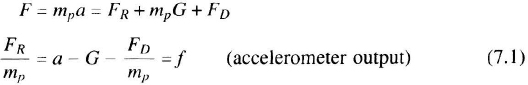
where F_R is the force exerted on the proof mass by the restoring spring or restoring amplifier, as shown in Figure 7.4, and F_D is the unwanted disturbing force caused by friction, hysteresis, mechanical damping, and the like. Thus, if the instrument is designed with negligible disturbing forces, the restoring force is a measure of (a − G) along the instrument's input axis. As explained in Section 7.5, accelerometers are used to calculate the vehicle's acceleration a; their outputs must be corrected for gravitation G in the computer.

Figure 7.3 Black-box diagram of an accelerometer.

Figure 7.4 Flexure-pivoted accelerometer.

If the accelerometer rests on a table, then a = 0 (neglecting the rotation of the Earth) and the unit measures −G. If the accelerometer is falling in a vacuum, then a = G, and the output is zero. If the instrument is being accelerated upward with an acceleration of 7 g, then a − G = 7 g − (−1 g), and the instrument reads 8 g (1 g is a unit of acceleration equal to approximately 32.2 ft/sec² = 981 cm/sec²; if an acceleration must be specified more exactly than 0.5%, it should be stated in fundamental units of length and time).

On the rotating Earth, a stationary accelerometer at a position R is accelerating centripetally at Ω × (Ω × R) in inertial space due to the Earth's rotation rate Ω. The accelerometer's output therefore measures Ω × (Ω × R) − G = −g, which is the ordinary definition of gravity, as discussed in Section 2.2. A stationary plumb bob on the Earth's surface points in the direction of g not G [24].

Construction Several accelerometer designs are used in aircraft inertial navigators:

1. Pendulum, supported on flexure pivots, electrically restrained to null.
2. Micro-machined (silicon) accelerometer with electrostatic nulling.
3. Vibrating beam accelerometer whose frequency of vibration is a measure of tensile force and hence acceleration.

The flexure-pivot accelerometer, shown schematically in Figure 7.4 is most commonly used in aircraft systems. The sensitive element consists of a pendulum with a torquer coil and pickoff supported by a torsional spring or flexure. The pickoff measures displacement of the pendulum from null and is often mechanized with an optical sensor and shadow mask or with capacitors. The torquer coils restore the pendulum to null, the torquer current being a measure of the restoring torque and, hence, of the acceleration. Mathematically, let f = a − G. The torque T on the pendulum is

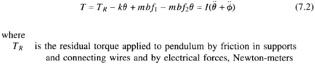
The damping is neglected for illustration. In the steady state

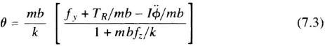
If the stiffness k is high enough, θ is small, and the instrument measures only f₁, independent of the presence of a cross-axis acceleration f₂. Sensitivity to f₂ is called cross-coupling and is most serious in a vibration environment when θ and f₂ oscillate in phase and rectify. This rectification is often referred to as vibropendulous error. The term T_R/k is the angle offset due to the presence of an unwanted torque on the pendulum; it causes an accelerometer bias. is an angular offset of the pendulum due to angular acceleration of the case around the pivot axis; is negligible when the accelerometer is mounted on a mechanical platform, but it is an important source of error in strapdown systems where and θ oscillations can rectify. If position calculations are referred to the center of percussion of the pendulum, the sensitivity to angular acceleration is reduced (see size effect. Section 7.4.1). The distance from the center of mass to the center of percussion is I/mb.

Flexure-pivoted accelerometers are simpler to construct than the older floated instruments since they do not require adjustment for buoyancy [23, pp. 288–289]. Because they are undamped, they exhibit high-frequency mechanical resonances. Resonances must therefore be controlled relative to both vibration inputs and rebalance-loop characteristics. Undamped accelerometers offer the greatest bandwidth (important for strapdown systems) but must almost always be supported on a shock-mounted sensor block (Section 7.4.1) in order to suppress high-frequency vibration and to prevent shock damage. Accelerometers that include fluid damping exhibit reduced bandwidth and additional thermal sensitivity due to changes in the fluid characteristics.

In navigation-grade accelerometers, a restoring loop maintains the pendulum near null. The restoring servo must be linear and repeatable from 10 to 25 µg to 40 g, a range of six to seven orders of magnitude. A digital output can be obtained by either digitizing the analog output (the current in the torquer coil) or by pulse-rebalancing with a digital restoring servo. When rebalancing with pulses of uniform height, pulse width measures incremental velocity ΔV. In either case, a properly initialized digital counter accumulates the pulses and stores the velocity change. The rebalance pulse train must not excite accelerometer resonances.

The pivot or flexure supporting the pendulum must provide minimal restraint for the pendulum in the direction of the input axis while exhibiting high stiffness in the other two directions. The spring constant of the pivot/flexure generates a restoring force that reduces the gain of the electronic restoring loop. The spring constant should be repeatable in order to ensure accuracy, but the high-stiffness restoring loop dominates. The pivot must not exhibit hysteresis, which may cause accelerometer biases. Generally, high-quality accelerometers can operate over wide temperature ranges (−55°C to 90°C) provided that temperature is measured and bias and scale factor are thermally compensated (Section 7.4.1) in the computer. Heating of the torquer coil due to rebalance current can lead to rectification of vibration inputs and must often be compensated. A pulse-rebalance torquer maintains constant heating.

A new generation of accelerometer employs silicon micro-machining [55]. A typical silicon accelerometer structure is shown in Figure 7.5. Single-crystal silicon forms the frame, hinges, and proof-mass. Anodic bonding joins this piece to metallized wafers which enclose the accelerometer and also serve as electrodes for sensing proof-mass motion and for rebalancing. Electrostatic centering of the proof-mass obviates the need for magnetic materials and coils. Due to the very small gaps achievable between the covers and the proof-mass, gas-film damping suppresses mechanical resonances. This permits the accelerometer to operate in high-frequency vibration environments.

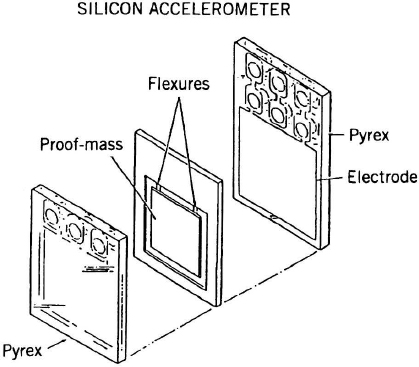
Figure 7.5 Silicon accelerometer (courtesy of Litton Guidance and Control Systems).

The silicon accelerometer can be rebalanced using either voltage or charge forcing. In voltage forcing, a potential is applied to the pendulum and to one or both electrodes. The voltages establish electric fields that induce charge on the nonconductive pendulum. This causes a net force to act on the proof mass. Thus, in the case of voltage forcing, the force generated is a function of the square of the applied voltage and of the gap between the pendulum and the electrode. Thus, non-linearities in force-versus-deflection may be incurred and may require compensation. The rebalance force can also be generated by applying charge to one or both electrodes of the device, by applying a precise current for a precise period of time. In the case of charge forcing, a fixed amount of charge generates a force that is independent of the pendulum's position, thereby permitting linear operation. However, proper charge metering requires complex electronics, particularly when small amounts of charge are to be transferred. Silicon accelerometers have less bandwidth than flexure-pivoted devices. An electrostatically induced spring rate results if the pendulum is not properly centered or if its position deviates from null. This causes scale factor or bias errors. A more detailed discussion of silicon accelerometers may be found in reference [55]. Silicon accelerometers are easy to manufacture using standard semiconductor technology, are rugged, and resist shock. In 1996, silicon accelerometers were used in some medium accuracy inertial measurement units (IMUs) and inertial-grade devices had been demonstrated.

Though the restrained-pendulum accelerometer is used in most operational aircraft inertial navigators, the micromachined vibrating beam or vibrating string accelerometer is sometimes used [38, 39], One version consists of a proof-mass that exerts a tension T on one or more vibrating beams (fabricated of metal, quartz, or other dimensionally stable materials). The frequency of oscillation of each beam is proportional to the square root of T, which varies with acceleration. By using two beams in push-pull, under an initial tension T₀, a frequency-difference measurement can determine acceleration:

If the tension T₀ is large in comparison with the maximum acceleration load mga, then the difference frequency is proportional to acceleration, with a decreasing series of higher-order corrections, in terms of odd powers of acceleration. The vibrating beam accelerometer requires a means of supporting the proof-mass in such a way that only the beam provides a support force along the input axis. Vibrating beam accelerometers are often sensitive to vibration and cross-axis inputs. One of their advantages is the ability of obtaining a digital output simply by counting the output frequency.

Multi-axis accelerometers that measure three components of acceleration with a single proof-mass have been developed. However, design difficulties exist in supporting the proof-mass and in constructing the geometry to keep inter-axis coupling sufficiently low; hence, these devices had not gained popularity in 1996. Unsuccessful attempts have been made to use the supporting force on a gyroscope to measure acceleration, thus converting the gyro into a combined gyro accelerometer. Other types of accelerometers, such as pendulous integrating gyro accelerometers (PIGAs) are used in space launch vehicles.

Error Model A typical error model for an accelerometer (including the restoring-amplifier electronics) expresses the steady-state instrument output u as

where

f1	is a component of a – G along the input axis
f2, f3	are cross-axis components of a – G
T	is the deviation from calibration temperature
D	is the dead zone, or threshold below which the instrument will not sense acceleration. This is typically caused by mechanical stiction and is much smaller than k0. This term is negligible in most modern inertial quality accelerometers.
H	is hysteresis (generally thermal)
ko	is the accelerometer bias (k0 is slightly different each time the instrument is powered-up; the mean value is usually biased out in the computer or the instrument itself; the uncompensated residual causes navigation errors.)
k1	is a linear scale factor, whose stability is essential in the design of the instrument
k1	is a nonlinear calibration coefficient (it is often desirable that this be negligible, in order to simplify the navigation algorithms)
k12, k13	are coefficients of cross-axis sensitivity
kθ	is the vibropendulous coefficient
θ	is the pendulum deflection angle
k41	is a linear temperature coefficient, for small deviations around the operating temperature

Dynamic rectification effects can also exist as a result of vibration and of saturation of the restoring amplifier. Typical accelerometer specifications control the values of k₁ and k₂ and their permissible variation due to temperature, vibration, cross-axis acceleration, and magnitude of input acceleration. Maximum values of D, H, k₂, k₁₂, k₁₃, k₄₁, and k_θ are usually specified.

Accelerometer Testing Accelerometers are statically tested and calibrated in the Earth's gravity field, using a dividing head. The dividing head causes the input axis to rotate in a vertical plane, around a horizontal axis, thus sensing a component of gravity that varies from 0 to ±1 g. Scale factor and bias are determined from such a test [Chapter 4 of Ref. 41]. Cross-axis sensitivity and variation of scale factor with cross-axis acceleration can be determined by tilting the pivot axis of the dividing head and repeating the test. To calibrate scale factor on a dividing head, a gravimetric survey should be performed at the calibration station. Without a survey, sea-level gravity can be predicted from Equation 2.6 within 0.02 cm/sec². Centrifuge tests are used to calibrate instruments that operate at acceleration levels greater than 1 g [61a,e]. Ref. 61h discusses precision centrifuge testing of accelerometers.

Aircraft instruments should be capable of operation at acceleration levels as high as 12 g (during military maneuvers) with an accuracy of better than 100 parts per million (ppm), if 1 nmi/hr navigation accuracy is to be achieved. The presence of vibration or shock on the sensor assembly requires that the accelerometer be scaled to sense considerably more than the maximum expected linear acceleration, in order to prevent saturation in the presence of acceleration combined with vibration. The accelerometer's frequency response can be restricted as long as the proof-mass does not strike the stops. Wide bandwidth is essential in accelerometers that input to a flight-control system or that are used to strapdown navigators.

The performance parameters of a typical aircraft accelerometer (circa 1996) scaled for 30-g maximum acceleration were the following:

D	negligible
H	25 µg
k0	25 µg (after thermal modeling)
k1	Stable to 50 ppm (after thermal modeling)
k2	< 5 µg/g2
k12, k13	Stable to within 25 µrad
kθ	< 2 µg/µrad-g
k41	30–100 µg/°C (stable to better than 0.5 µg/°C)

7.3.2 Gyroscopes

Purpose The purpose of the gyroscopes (“gyros”) in an inertial navigation system is to space-stabilize the accelerometers. In gimballed platforms, the gyros measure rotation of the platform, which is angularly isolated from the vehicle's motions. The gyros rotate at inertial angular rates from 0.005 deg/hr to 50 deg/hr, the maximum torquing rate on fast aircraft; a range of 10,000. The gyroscopes are used as error detectors to sense small rotations of the platform relative to the navigation coordinates. A gimbal servo-loop restores the error to near zero (see Figure 7.2 and Section 7.4.2).

In strapdown systems, the gyroscopes are fixed to the vehicle and follow its angular motion. A gyroscope on a military aircraft must sense angular rates as low as 0.005 deg/hr and as high as 400 deg/sec (1,440,000 deg/hr), a range of 8.5 orders of magnitude. Strapdown gyroscopes on civil aircraft need only sense an 8-order-of-magnitude range of angular rates.

Construction Many types of gyroscopes have been invented. Since the 1930s, directional gyroscopes have been used in cockpits as heading references (Chapter 9). They are spinning-wheel, large-angle, unfloated instruments with ball bearings that have drift rates on the order of 50 deg/hr, and hence are useless for navigation.

From the 1940s to the 1960s, single-degree-of-freedom (SDF) floated gyros were perfected. A spinning wheel was mounted inside a single gimbal that was floated at neutral buoyancy. A magnetic pickoff sensed rotations (several minutes of arc) and a magnetic torquer precessed the rotor according to a rebalance algorithm. These gyros achieved drift rates less than 0.01 deg/hr but had to be used on a stable element since they were very sensitive to cross-coupling. They were used principally in space launch vehicles [61b].

From the 1950s to the 1970s, floated two-degree-of-freedom (TDF) gyroscopes were perfected for aircraft. A spinning wheel was mounted in two gimbals and floated at neutral buoyancy. Two orthogonal pickoffs (usually magnetic) sensed rotation of the float and two orthogonal torquers (also magnetic) precessed the float according to a rebalance algorithm. These gyros achieved drift rates of 0.01 deg/hr and were almost always used on a gimballed platform. The motors, fluids, and seals caused perennial maintenance problems. These instruments were described in the first edition of this book [23].

During the same period, electrostatically suspended TDF gyroscopes were developed for submarines [56]. Their spinning wheels are electrostatically centered, achieving 0.001 deg/hr accuracy but at costs orders of magnitude higher than floated TDF gyros. Due to their high accuracy, electrostatic gyroscopes are used for high-precision, deep-penetration, long-time-of-flight aircraft. Hydrostatically suspended gyros, using pressurized bearings to support the gimbals, were also developed but little used.

From the 1970s to the 1980s, “dry-tuned” or “tuned-rotor” or “dynamically tuned” gyroscopes were perfected, as described in Section 7.3.4. Navigation gyros of this type have insufficient range for strapdown use and were mostly used in gimballed platforms. Strapdown tuned-rotor gyros were used in 1996 for lower-cost, moderate accuracy attitude and heading reference systems (AHRS), which also serve as coarse navigators (Chapter 9 and Section 7.7.4).

In the 1980s, optical angular sensors were perfected after 30 years of development. They are the mainstay of aircraft inertial navigators in the 1990s and are described in Section 7.3.3. These instruments are called gyroscopes to emphasize their function. Research efforts on new gyros are described in Section 7.3.5.

7.3.3 Optical Gyroscopes

Optical gyroscopes were universally used in strapdown aircraft inertial navigators in 1996. These gyros offer extremely high dynamic range, linearity, bandwidth, ruggedness, and reliability. By the 1980s, most of the key problems inherent in the ring laser gyro (RLG) had been solved or circumvented. Thus, the RLG surpassed the mechanical gyro as the rotation sensor of choice for inertial navigation systems. Strapdown RLG systems have become the predominant inertial navigators for commercial and military aircraft. New generations of laser gyroscopes have also been developed. These include multioscillator laser gyros that employ optical biasing as a means of circumventing lock-in (a key limitation in laser gyros), and fiber-optic gyros. All optical gyros make use of the Sagnac effect, a relativistic phenomenon that permits the observation of rotation relative to inertial space. Optical gyros can be configured as resonators or as interferometers, as discussed below. Systems designed with optical gyros are much simpler than those using mechanical gyros.

The Sagnac Effect The Sagnac effect [43] is a general relativistic phenomenon relating to the propagation of light in a rotating reference system. When laser beams circulate in a closed path that is rotating in inertial space, the optical length seen by the co-rotating beam appears longer than that seen by the counter-rotating beam. The Sagnac effect permits observation of rotation in one of two different ways.

• In a resonator (such as an RLG), the counterpropagating beams form resonant modes within the cavity. These create an electromagnetic standing wave that remains fixed in inertial space [1]. When the housing of the gyro rotates, a detector can count nodes of the standing wave, each of which represents a fixed increment of angle (see Figure 7.7).
• In an interferometer, counterpropagating beams are launched into an optical path and recombined as they exit. The interference generated by the recombination depends on the optical phase difference (proportional to the optical path difference) between the two beams and therefore provides a measure of rotation. In 1996 most fiber optic gyros were configured as interferometers. Fiber-optic gyros may also be constructed as resonators but the absence of a gain medium and the relatively high losses of the fiber rendered this type of device impractical in 1996.

Two-Mode Ring Laser Gyros The RLG has undergone extensive development since the late 1970s. In 1996, the two-mode RLG [8, 59] was the most prevalent optical inertial sensor, although multioscillator gyros were penetrating the marketplace as fully strapdown sensors (i.e., no dither). The conventional two-mode and the multi-oscillator gyros subscribe to many of the same principles but also differ in fundamental respects.

Two-mode RLGs (Figure 7.6) are planar by design so that only linearly polarized modes can be resonant in the cavity. Suppression of one of the two polarizations ensures stable operation. The two-mode RLG therefore employs a single linearly polarized clockwise (cw) and a single linearly polarized counterclockwise (ccw) beam. Higher-order modes are suppressed through proper alignment and apertures. A block of glass is bored to form a three-or-more-sided polygonal path. High-quality mirrors at each vertex complete the resonant cavity. The bores are filled with a gas mixture (generally helium and neon) that serves as a laser gain medium. The laser is excited by an electrical discharge-generated by one or more cathodes and one or more anodes in contact with the gas. The laser beams that resonate within the cavity are electrically “pumped.” A high gain-to-loss ratio permits the RLG to achieve good accuracy.

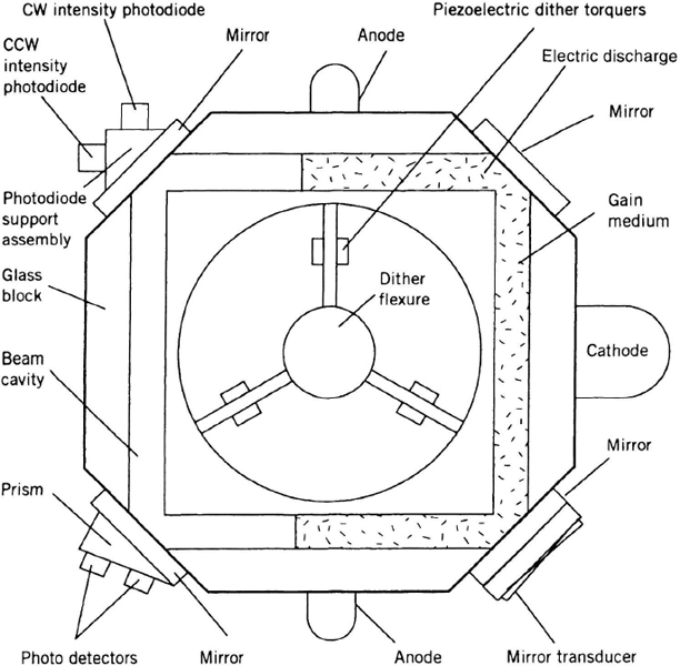
Figure 7.6 Two-mode ring laser gyro (courtesy of Litton Guidance and Control Systems).

The RLG provides an angle readout via a partially transmissive mirror at a vertex. A set of combining optics (typically a prism) coherently recombines (heterodynes) the clockwise (cw) and counterclockwise (ccw) beams in order to permit the observation of the standing-wave pattern (also referred to as interference fringes) created by the counterpropagating modes. Photoelectric detectors measure the intensity of the interference fringes.

As discussed in the previous section, the standing-wave pattern does not rotate in inertial space. Thus, rotation of the RLG relative to the standing wave may be observed as a change in intensity sensed by the body-fixed detectors, as illustrated in Figure 7.7 for a fictitious “circular” RLG. In this figure, two counterpropagating waves create a standing-wave pattern. When the gyro is rotated, the detector moves with respect to the interference pattern and senses dark and light areas. Each dark/light cycle represents one-half wavelength of the laser beam along the circumference of the path. The number of dark/light transitions can therefore be geometrically related to the angle of rotation as indicated in Figure 7.7. The count of transitions yields the total rotation angle. At a typical laser wavelength of 630 nm, each dark/light cycle would represent one arcsecond of rotation for a 5-cm radius ring. The scale factor of the instrument depends on the ratio of enclosed area to path length, as shown in Figure 7.7 for the “circular” RLG. A similar analysis can be made for any closed polygonal laser path:

where

A	is the enclosed area of the laser path
L	is the path length of the laser beam
λ	is the wavelength of the laser
Δθ	is the rotation angle increment
Nfringes	is the number of fringes traversed, measured in units of half a wavelength

RLG Quality The laser is based on stimulated emission of photons. However, the gas medium that supplies the gain for the laser also occasionally emits photons which are unrelated to the laser signal. This is known as spontaneous emission, and leads to noise and random walk in the RLG angle output. Spontaneous emission is described statistically through quantum mechanics and cannot be eliminated. To reduce its impact on gyro performance, the active signal must be as large as possible. A gyro with high gain and low loss is said to have a high “finesse” (analogous to Q in a resonator). To increase finesse, it is important to incorporate high-quality mirrors into the RLG. Low loss minimizes the impact of spontaneous emission and reduces the “quantum limit,” which is a measure of the best noise performance (and hence angle random walk) achievable with the gyro.

Figure 7.7 Circular ring laser gyro.

For reasons discussed below, it is essential to minimize the backscatter generated by the mirrors. Greater angle of incidence leads to decreased backscatter. A trade-off must be made between the number of mirrors used and the resulting angle of incidence. For example, a three-sided gyro employs only three mirrors but exhibits a 30-deg angle of incidence while a four-sided gyro has a more favorable (45-deg) angle of incidence but requires a fourth mirror with its attendant losses. Gyros with more than 4 sides are not made.

Lock-in The most severe problem encountered in the RLG is that of lock-in. In the 1960s, it was observed that the RLG was insensitive to low angular rates, as illustrated in Figure 7.8. The cause of the lock-in phenomenon is backscatter within the cavity, usually resulting from imperfections in or particulates on the mirror surfaces. At low rates, the two counterpropagating beams in the resonator are very close in frequency (less than a few hundred out of 5 × 10¹⁴ Hz) because their optical path lengths are nearly equal. Coupling of one beam into the other (which results from backscatter) causes the two modes to “lock,” together thereby making the gyro insensitive to the actual rate. In Figure 7.7, backscatter amounts to friction between the standing-wave pattern and the cavity. When the gyro is rotated at low rates, the standing-wave pattern “sticks” to the cavity instead of remaining fixed in inertial space. The detector therefore does not shift with respect to the interference fringes, and the gyro does not observe the rotation. At high rates, the “friction” is overcome because the frequencies separate and the gyro is capable of measuring rate.

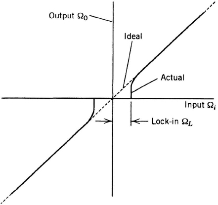
Figure 7.8 Two-mode RLG input/output (no dither).

In a two-mode RLG, mechanical biasing is employed to overcome lock-in. The usual means for accomplishing this is mechanical “dither,” which is a large-amplitude sinusoidal motion applied to the gyro body. Typically, peak dither rates are 100 deg/sec. The output of the gyro must then be compensated for the dither motion so that the true rotation of the vehicle can be determined. There are many effective techniques for compensating. One of the drawbacks of dither is increased random walk. As the sinusoidal motion crosses through zero velocity, a small lock-in error occurs. Since the gyro reverses direction twice per dither cycle, these errors accumulate as a random walk process. Dither-induced random walk decreases with the square root of dither rate but is usually the dominant source of random walk.

An alternative method (which avoids the random walk problem) of biasing the RLG employs a turntable that applies a constant rotation to the gyro. An angular encoder measures the relative angle between the instrument and its base. This technique is referred to as rate biasing. Rate-biased systems with small-path-length RLGs have been delivered for missile applications. High-performance systems also use this method in order to avoid excess random walk, to provide partial error cancellation as the instruments rotate in space, and to improve calibration [35]. Because of the mechanical complexity involved in rate-biased systems, they are rarely used in aircraft.

Mechanical Design Most RLG systems in 1996 employed dither to circumvent lock-in. However, dither places serious constraints on the mechanical design of the system. High-frequency (typically several hundred Hertz), high Q mechanical flexures apply the dither. Coupling of dither to mounting structures has many undesirable effects such as acoustic noise, vibration, and energy loss. Thus, hard-mounted dithered systems are generally not practical and a low-frequency suspension (typically 30 to 50 Hz) isolates the sensor assembly from the aircraft. Dither torques in the three instruments excite coning rotations (discussed in Section 7.4.1), which cause errors in the navigation of the block solution [20]. Coning drift increases as the square of dither amplitude.

Cavity Length Control The RLG operates as a resonant cavity. The gas mixture, which sustains the laser, exhibits gain at certain optical frequencies that excite the stimulated emission, resulting in lasing action. Therefore, the length of the cavity must be tuned to be an integral number of wavelengths. For a helium-neon gas mixture, the wavelength is approximately 630 nmeters. Obviously, a cavity whose length is accurate and stable to 1% of a wavelength would be impractical to design. Thus, cavity length is controlled actively by continuously adjusting mirror positions in order to maximize total laser intensity. Piezoelectric transducers mounted on the back of one or more mirrors induce minute displacements of the mirror faces.

Since mirrors can only move a few wavelengths, the cavity must be made of a low-expansion glass so that the mirror travel is sufficient to compensate for expansion over the entire temperature range. Otherwise, “mode hops” must be performed, wherein the path length of the gyro is quickly changed by one wavelength to another control point. Unfortunately, data are lost or corrupted during a mode hop. Frequent mode hops or mode hops during high dynamics must be avoided. Unless low-expansion glass is used, mode hops could occur as frequently as once every 3°C.

Gas Mixture The RLG cavity should be designed to avoid gas flow within the cavity. A net gas flow causes gyro bias and can be a dominant error source in any RLG. To reduce flow, the temperature gradients across the glass block should be limited to 1–2°C.

Because of their small size, helium atoms diffuse easily into many materials. In very small RLGs, the volume-to-surface ratio is low and, helium diffusion limits gyro life. The glass that forms the laser cavity must have low thermal expansion and low helium permeability.

RLG Scaling Laws The performance of a ring laser gyro depends on its size. The parameters that describe gyro performance include the random walk coefficient, bias stability, resolution (also known as quantization), and scale factor stability. Because the ratio of area enclosed by the beam to path length determines the sensitivity of the gyro, most of the performance parameters improve with path length. The following scaling laws are provided as guidelines:

Reference [59] provides a more detailed discussion of error sources and mechanisms. Due to the strong path-length dependencies, quality (particularly of mirrors) becomes more critical as path length is reduced. Thus small RLGs, while offering packaging advantages, generally do not provide cost advantages.

Vibration Sensitivity Although the laser is insensitive to vibration, the RLG may have dynamic errors. For example, if the RLG flexure (which permits dither) exhibits cross-axis compliance, then the three gyros in an inertial system no longer form a rigid body, and large navigation errors may result during vibration. The flexure design must be compliant (with a very high Q) about the input axis while being extremely rigid about the other two axes. An angular pickoff senses the dither motion thereby correcting for dither. Still, vibration-induced errors will result if the pickoff mechanism is sensitive to translational acceleration.

For example, if the strain sensors that measure dither are slightly asymmetrical, they will erroneously indicate an angular motion of the gyro. If the false angular signal is synchronous with a true angular motion about a perpendicular axis, the strapdown equations will generate a coning-like error which is called pseudo-coning.

Multioscillator Gyro The two-mode RLG requires dither or turntable rotation, imposes constraints on the mechanical designs, and causes increased noise (both vibratory and acoustic), random walk, and coning. Therefore, methods of optically biasing ring laser gyros have been attempted since the 1960s. This has led to the class of RLGs known as multioscillators [49]. These are fully strapdown, wide bandwidth, high-resolution, angle-sensing devices. They have no moving parts and generate no acoustic noise. A description of their operation is given below.

Construction In one form of multioscillator RLG, a left-hand circularly polarized (LCP) mode and a right-hand circularly polarized (RCP) mode are each split apart in frequency creating two gyros acting within the same resonator. The LCP and RCP modes are separated with an optically active crystal that rotates polarization states and consequently introduces a differential phase between the LCP and RCP waves (reciprocal splitting) [49]. A more attractive alternative makes use of an out-of-plane geometry that causes polarization rotation. This is likened to the rotation of an image as it is subject to a series of reflections. The geometric technique of polarization separation is preferred, since it does not require the addition of a crystal within the beam path.

Once the LCP and RCP modes are split, they may be treated as two separate gyros each possessing clockwise and counterclockwise beams. As such, lock-in may occur in each of the gyros thereby precluding low-rate measurements. To avoid this, the clockwise beam is biased away from the counterclockwise beam. This can be accomplished with a doped glass element in the beam path which, when subjected to a magnetic field, causes a differential phase shift between the clockwise and counterclockwise beams. The shift is in opposite directions for the LCP and RCP modes. The phenomenon responsible for the phase shift is known as the Faraday effect, and the glass element that produces it is known as a Faraday rotator. The frequency splitting in a multioscillator gyro is illustrated in Figure 7.9a. It is noted that in this multioscillator, four laser modes simultaneously resonate within the cavity.

As illustrated in Figure 7.9b, when a mechanical rotation is applied to the multioscillator, the rate sensed by one of the two “gyros” (LCP in Figure 7.9) increases, while the rate sensed by the other “gyro” (RCP in Figure 7.9) decreases. The subtraction of the two gyro outputs cancels the Faraday bias while doubling the true angular rate measurement. The multioscillator readout is much the same as that of the RLG except that two sets of fringes (one from each polarization) are counted. The difference in the number of fringes is proportional to the rotation angle. The resonant multioscillator cavity resembles a conventional RLG cavity but must have at least four sides arranged so that the beam does not circulate in a plane. A Faraday rotator lies within the beam path and a magnet applies the field required to generate the Faraday rotation. Figure 7.10 depicts such a multioscillator gyro. As with conventional RLGs, cathodes and anodes support the electric discharge, which pumps the laser, and combining optics detects the interference fringes.

Figure 7.9 (a) Mode splitting in a multioscillator RLG; (b) effect of rate on multioscillator RLG.

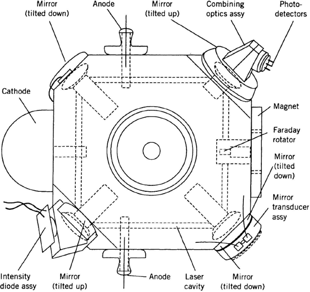
Figure 7.10 Multioscillator RLG (courtesy of Litton Guidance and Control Systems).

While lock-in is avoided in multioscillators, other difficulties arise. Interaction between scatter sources on the surfaces of the Faraday rotator and of the mirrors causes mode coupling, which can lead to increased gyro bias. High-quality mirror and rotator coatings minimize this problem. To ensure cancellation of common mode errors, it is important to balance the LCP and RCP intensities. This may be accomplished by dynamically adjusting the cavity length either to maximize total gyro intensity or to control the difference between the LCP and RCP intensities.

The elimination of mechanical dither makes the multioscillator gyro exceptionally well suited for low noise, flight control, and pointing applications. The elimination of dither leads to a low random walk coefficient. The scale factor stability is exceptionally good due to the absence of scatter-induced lock-in effects present in dithered gyros. The doubling of the scale factor allows smaller instruments to be used, and the lack of dither-induced mechanical noise permits superior angle measurement and enhanced flight control potential. The mechanical designs are simplified due to the absence of high-frequency, high-Q dither flexures.

Fiber-Optic Gyro Fiber-optic gyros (FOGs) may be constructed as resonators (much as RLGs) or interferometers. Resonant FOGs have been attempted but suffered from a high loss-to-gain ratio and excessive scatter. In 1996, most operational FOGs were interferometers [11].

Principle of Operation The interferometric fiber-optic gyro (IFOG) consists of a light source, a coupler, a fiber coil, and a detector as shown in Figure 7.11. Light is launched from a broadband laser source and coupled through a fiber-optic coil in both the clockwise and counterclockwise directions. Because of the Sagnac effect, the optical paths seen by the two beams differ in proportion to the angular rate applied to the gyro. Upon recombination, the two beams interfere and the intensity measures the phase difference between the beams. Reference [32] shows that the phase difference is proportional to

Figure 7.11 Interferometric fiber-optic gyro.

where ω is the instantaneous inertial angular velocity along the axis of the coil and T is the time for the light beam to traverse the coil. Thus, the fiber-optic gyro's output characteristic is that of a rate-integrating gyro with a short memory as opposed to a ring laser gyro, which is a rate-integrating gyro over a longer period of time (i.e., as long as interference fringes are being counted).

Fiber-Optic Gyro Modulation In an interferometer, small phase shifts (corresponding to low angular rates) cause minute intensity changes (see Figure 7.12). To increase the rate sensitivity, it is necessary to modulate the fiber-optic gyro so that the phase shift between beams is an odd multiple of π/2. In early FOGs, the beams were phase-modulated mechanically by the piezoelectric mandrel that served as the spool for the fiber-optic coil. An electrical excitation applied to the piezoelectric material stressed and stretched the optic fiber, thus causing a change in its index of refraction. The result was a modulation of the beam phase in the fiber. The development of integrated optics permits the replacement of the piezoelectric mandrel with an electro-optic modulator within the beam path as shown in Figure 7.13. Light passing through the modulator is phase-shifted in proportion to the voltage applied. Modulation must be applied with a period approximately equal to the transit time. A detailed discussion of FOG modulation may be found in reference [52]. It may take the form of a sinusoidal wave form, but, in 1996, state-of-the-art devices often employed complex digital modulation to achieve maximum sensitivity and to avoid problems with distortion.

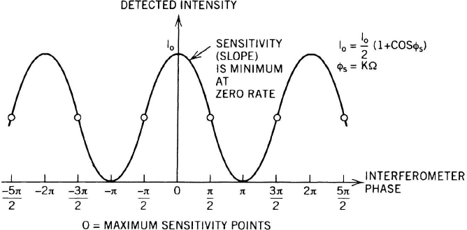
Figure 7.12 Detected intensity versus interferometer phase.

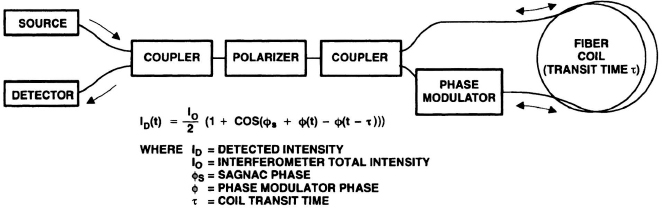
Figure 7.13 IFOG with phase modulator.

Closed-Loop Fiber-Optic Gyro Operation Gyro modulation improves sensitivity at low rates. However, electronics nonlinearity, intensity variation, photodetector sensitivity, preamp gain, and background intensity all contaminate the open-loop output of the FOG. For this reason, closed-loop operation of the FOG is advantageous for higher accuracy and greater dynamic range [52]. Angular-rate-induced phase shift may be nulled by applying a phase rebalance with the modulator. However, the modulator is not selective as to direction of beam travel. A step voltage applied to the device will sustain a differential phase shift between the clockwise and counterclockwise beams for one transit time of light through the coil. A steady-state voltage will result in no net steady-state differential phase. A persistent differential phase can only be generated by a repeated increase in the voltage applied to the modulator. Thus, to null the rate-induced shift with a phase modulator, it is necessary to increase the voltage applied at least every transit time. Since available voltages are bounded, the phase cannot increase indefinitely. Thus, periodic voltage “resets” (of sub-microsecond duration) with corresponding phase magnitude of 2π are applied to maintain the voltage supplied to the phase modulator within prescribed limits. The magnitude of each reset must be exactly 2π of phase to ensure that the gyro is not perturbed. A block diagram of a typical closed-loop FOG mechanization is given in Figure 7.14. As in the case of modulation, a digital implementation of the rate rebalance loop is attractive because it permits more precise control, tracking, and integration of the rate rebalance signal. Control of the reset amplitude is usually accomplished through the use of a secondary servo, which compares the effect of a nominal π/2 step to that of triple the nominal step. If the step were exactly π/2, the triple step would be −3π/2, which should have the same effect. However, if the step was not exactly π/2, the difference between the step and triple step would adjust the voltage on the phase modulator to achieve π/2 [52].

Figure 7.14 Closed-loop FOG operation.

Polarization Nonreciprocity The construction of the fiber-optic gyro usually leads to a high degree of reciprocity. That is, in the absence of external influences (angular rate, modulation), the clockwise and counterclockwise beams each experience equal phase shifts, leading to zero differential phase. However, one common error source, which may be nonreciprocal, is the coupling of different polarizations within the fiber/coupler circuit. Such coupling is usually highly temperature-dependent and cannot be modeled. Polarization nonreciprocity must be minimized through the use of high-quality polarizers, short-coherence-length sources, and polarization-maintaining fiber and/or depolarizers. In 1996, most fiber-optic gyros employed a broadband source such as a superluminescent diode (SLD) or an active gain fiber source. Narrow-band laser diodes are generally unsuitable for use in FOGs.

Vibration/Thermal Sensitivity The index of refraction and the physical length of the fiber-optic gyro coil are affected by ambient temperature and pressure. These cause a rate error known as the Shupe effect. Thermal Shupe effect leads to a gyro bias that is a function of temperature and temperature gradient changes, while mechanical Shupe effect converts periodic translational vibration into periodic angular rate. Both of these effects may be reduced through clever coil-winding methods. Thermal compensation may further improve performance.

Electronics Short-fiber-length (50 to 1000 meters) gyros require fast electronic components that generate modulation, process data, and rebalance the gyro phase. Digital modulation, demodulation, and loop-processing are the most effective.

Advantages of Fiber-Optic Gyros The FOG requires no mechanical biasing and is rugged enough to be operated in a hard-mounted configuration. Short-fiber-length FOGs offer small size, weight, and cost. The fiber-optic gyro provides extremely fine quantization (<0.01 arcsec) thereby permitting its use as a rate-integrating device and as a low-noise rate sensor. In 1996, one-deg/hr FOG systems were in production for attitude and heading reference systems (AHRS) [36]. They are adequate for many GPS-inertial systems. Navigation-accuracy FOGs have also been produced and demonstrated.

Size, Weight, and Performance In 1996, optical gyros suitable for inertial navigation weighed from 500 to 2000 g per axis. Laser gyros employed path lengths of between 15 and 35 cm, while navigation-grade fiber-optic gyros utilized approximately 1 km of fiber. In most cases, optical gyros are sold with their supporting electronics. The drift rate of an optical gyroscope is given by

The sources of error are classified below. The Ω_i are the components of angular rate about orthogonal system axes and T is the difference between the operating and calibration temperature of the gyro.

Bias and Random Drifts Bias terms C₀ and C₁ are driven by gas flow effects in RLGs, scatter effects in multioscillators, and polarization and electronics effects in FOGs. They change with age but bias is extremely stable from turn-on to turn-on. Long-term bias aging is usually compensated in a system using Kalman filter observations of bias error (Section 7.7.3). Thermal hysteresis H may be incurred due to the buildup of gradients or stresses in the gyros during thermal cycling.

Deadband The deadband or threshold term D specifies the rate below which the gyro is insensitive. It is due to lock-in in RLGs and electronics errors in FOGs.

Scale Factor and Nonorthogonality In laser gyros, scale factor error M₁₁ is due to mode coupling effects and is usually negligible, limited only by the accuracy of calibration. In FOGs, scale factor error is driven by the wavelength of the light source and the index of refraction of the fiber. Nonorthogonality errors M_ij are due to mechanical misalignment between the gyros and the sensor assembly. Compensation of nonorthogonality is performed in the system computer.

Magnetic Sensitivity Magnetic sensitivity k_ij is due to the interaction of magnetic fields with polarization states and with the propagation medium. Laser gyros and FOGs are usually enclosed in a high-permeability shield that attenuates external magnetic fields.

White Noise The white noise W of an optical sensor is usually a significant error source. Noise due to spontaneous emission of photons in light sources and due to backscatter in dithered RLGs sets the ability to measure the gyro output within a set period of time. For example, a gyro whose power spectral density of rate noise is 0.12 deg/hr-√Hz will measure angular rate with a standard deviation of 0.0055 deg/hr when using an integration time of eight minutes. Rate noise can be converted to angle noise by dividing by 60. Thus, a spectral density of (0.12 deg/hr-√Hz) is equivalent to an angle spectral density of (0.002 deg/√hr)².

After compensation, the residual errors are given by

Testing Optical gyroscopes are tested using rate tables with thermal chambers to measure scale factor and bias at various temperatures. Testing is simplified due to the excellent scale factor stability of these gyros. Vibration testing is sometimes performed to verify construction quality and durability and to measure vibration rectification errors. Ref. [61i] describes test procedures for single-axis laser gyroscopes.

7.3.4 Mechanical Gyroscopes

Prior to the advent of the optical gyroscope, mechanical devices formed the basis of inertial navigation systems. References [47, 23] describe various types of mechanical gyroscopes.

Spinning Wheel Gyros The principle of operation is that in the absence of applied torque, a rapidly rotating mass will tend to maintain its orientation in inertial space. If a torque acts on the mass, then it will precess at a constant rate. If a rigid body of angular momentum H (H = Iω_s, where I = moment of inertia of the mass about the axis of rotation, and ω_s = spin rate) were acted upon by a torque T, then the body would precess at an inertial angular velocity ω:

where

Ti	are components of the applied torque
A	is the rotor transverse moment of inertia
C	is the rotor polar moment of inertia
H	is the angular momentum of the rotor
ωi	are the case angular velocities in inertial space
θi	are the pickoff angles

Figure 7.15 Black-box model of mechanical gyroscope.

If the angular momentum is high enough, Equation 7.9 can be simplified as represented in Figure 7.15:

The simplification neglects anisoinertia (C-A), mass unbalance, and gimbal moments of inertia. Many of these effects must be considered particularly in strapdown systems that experience high dynamics and change their orientation with respect to gravity. Other errors are present at higher frequencies where the rebalance loops cease to faithfully maintain the rotor at its null position. Detailed discussions of errors may be found in references [9, 10].

Equation 7.10 shows that a torque applied around an axis perpendicular to the spin axis generates a precession rate T/H around an axis perpendicular to the other two. By definition, the rate ω resulting from a deliberately applied torque is called a precession, whereas that due to an accidentally (and unwanted) applied torque is called drift.

If a constant torque were applied to a nonrotating mass, the result would be a constant angular acceleration T/I. After a time t, the nonrotating mass would turn through an angle Tt²/2I, whereas the gyro would turn through Tt/Iω_s. By increasing the spin rate ω_s, a gyro can be made much stiffer than an inert mass of the same moment of inertia. References [48, 51] discuss the dynamics of mechanical gyros in great detail.

Tuned-Rotor Gyros Figure 7.16 schematically illustrates a two-degree-of-freedom (TDF) gyro. A balanced rotor supported in flexure-gimbals is free to rotate about two axes relative to the shaft. Preloaded bearings support the shaft within the case and a motor drives the rotor at a precise spin speed of approximately 200 revolutions/sec. Pickoffs (usually magnetic) measure the angular displacements (θ_x and θ_y) of the rotor relative to the case. Mechanical stops prevent damage to the gyro due to excessive motion of the rotor. The pickoff outputs drive servo loops, which control torquers that restore the rotor to its null position. The gyroscopic equations relate the torque applied (measured by the current supplied to the torquer coils) to the angular rate sensed by the gyro. Angular rate measurements about two perpendicular axes are obtained. Additional descriptions of tuned-rotor gyro design are given in reference [31].

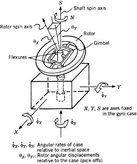
Figure 7.16 Schematic representation of TDF tuned-rotor gyro.

Suspension Tuning The suspension includes a gimbal and two sets of flexures. Its function is to provide translational support for the rotor while decoupling the case and the rotor for rotations about any axis perpendicular to the spin direction. When the gimbal-flexure-rotor assembly spins, a dynamically induced spring rate is generated [10]. The tuned condition is achieved when the dynamic spring rate exactly cancels the mechanical spring rate attributed to the flexure. The gimbal inertias are adjusted such that their tuned frequency exactly matches the motor frequency. When ideally tuned, the rotor will appear to be completely free to rotate about axes perpendicular to the spin axis.

Rebalance Servo To keep the gimbal angles within seconds of arc, a rebalance servo drives the pickoff signals to zero. Magnetic torquers act on the rotor to provide the restoring force. As in the case of accelerometers, the rebalance loops can be analog or digital (pulse rebalance). Gyro resonances and rebalance loops must be designed to achieve sufficient bandwidth while ensuring stability. Torquer calibration includes orthogonalization relative to the gyro spin axis and relative to the other torquers. In older designs, such calibration was generally performed electrically with a resistor matrix. Newer instruments rely on mathematical compensation in the navigation computer.

Torquing of strapdown gyros is difficult for several reasons. To achieve high rate capabilities and high bandwidth, either large torquers must be used or a rotor with low inertia must be used; both degrade performance. In the first instance, excessive power dissipation, thermal sensitivity, and thermal gradient sensitivity cause drift. In the second case, accuracy is sacrificed because of the reduced gyroscopic effect. The angular momentum of inertial-quality gyros is 200,000 to 2,000,000 gm-cm²/sec. For strapdown navigation, optical gyros (Section 7.3.3) have nearly displaced mechanical gyros. Lower-accuracy strapdown inertial measurement units still employ miniature two-degree-of-freedom-tuned gyros.

Size, Weight, and Performance Inertial-quality TDF gyros range from micro-machined 30-g instruments to 300-g tuned instruments excluding power supplies and control electronics. They consume milliwatts to 5 w. The drift rate of one axis of a mechanical gyro can be represented as

The sources of error are classified below. The a_i are the components of case acceleration along the spin axis and gimbal axes of the gyro, T is the difference between the operating and calibration temperature, and the B_i are the components of the ambient magnetic field.

Bias and Random Drifts Bias drift C₀ is caused largely by suspension torques and by the back reactions of pickoffs. The bias drifts differ slightly each time the instrument is turned on (day-to-day and long-term repeatability) and will fluctuate randomly with time because of pivot friction, pigtail hysteresis, brinelled bearings, and power supply variations. A turn-on to turn-on bias shift can result from the way in which the shaft bearings align themselves at each spin-up. Bias and random drifts are specified in deg/hr. Mechanical gyros in aircraft are usually rebiased on a regular schedule, based on the number of flights, flying hours, or elapsed time. In most systems, biases are estimated in flight by the navigation Kalman filter (Chapter 3).

Mass-Unbalance Drift The C₁, C₂, and C₃ are the mass-unbalance drift coefficients. Mass-unbalance drift is proportional to vehicle acceleration and is caused by inadequate mass balance of the assembly or by a defective spin motor. If H = 2 × 10⁶ g-cm²/sec and the rotor weighs 250 g, a mass shift of 1 µin. causes a drift coefficient of 0.06 deg/hr-g. The absolute values of C_i and their stability are usually specified. Compensation is sometimes performed in the system computer using accelerometer measurements.

Anisoelastic Drift The C₁₂, C₁₃, and C₂₃ are the anisoelastic drift coefficients, usually specified in deg/hr-g². If the wheel suspension is not isoelastic, the mass center of the rotor does not deflect along the direction of acceleration and a torque results. A difference in stiffness of 1 1b/µin. will cause a drift coefficient of 0.04 deg/hr-g² if H = 2 × 10⁶ g-cm²/sec and the rotor weighs 250 g. Furthermore, a vibration that has in-phase components along and normal to the spin axis will cause rectified drift.

Higher-Order g-Sensitivity If the deflections along the principal axes are nonlinear functions of load, the anisoelastic drift coefficient will vary with g³ and higher-order terms. These terms are not ordinarily discernible in aircraft systems.

Temperature Coefficient of Drift The temperature-dependent drift in a gyro results from dimensional changes in the mechanical assembly or temperature dependent terms in the magnetics. These coefficients are quoted in deg/hr-°C of temperature off calibration and of the temperature gradient. For maximum accuracy, mechanical gyros are often heated and maintained at a precise temperature. A temperature model can also be derived during calibration and subsequently applied in the system computer for drift compensation.

Magnetic Field Coefficient of Drift External magnetic fields can act on the motor or suspension causing torques that depend on the field strength and on the orientation of the gyro in the field. The source of the field can be the Earth, nearby equipment (e.g., radars), platform torque motors, or sources within the gyro. The magnetic field coefficient is quoted in deg/hr-gauss.

In a typical navigation-grade mechanical gyro (circa 1996), the coefficients in field usage are

Testing There are many methods for conducting static drift tests on gyros. In the simplest, the gyro is mounted on a rigid table and connected as a single-axis or two-axis rate gyro, with its pickoff(s) caged to its torquer(s). The indicated gyro output expressed as a rate, minus the calculated Earth rate, gives the drift rate. This method depends on knowledge of the torquer scale factor and requires the subtraction of two large numbers to calculate the small drift rate. This test is usually performed on mechanical aircraft gyros because they have calibrated torquers and because the test maintains the gyros in a fixed orientation relative to gravity. Measurements of the gyro drift rates in various orientations relative to the gravity field can be used to solve a set of simultaneous equations of the form of Equation 7.11 to yield the drift coefficients in that equation [61g].

Vibration tests of a gyro are often desirable, particularly to determine the anisoelastic coefficients, which are a function of the frequency of vibration. Centrifuge tests also characterize gyros but are difficult to perform accurately. Sled tests and Scorsby tests (Section 7.4.3) are used to test strapdown blocks but not individual gyros.

7.3.5 Future Inertial Instruments

For precise inertial navigators (better than 2 nmi/hr RMS error), optical gyroscopes are likely to remain in use for decades. Efforts will continue to avoid mechanical dithering and to improve the reliability of the laser cavities. Approaches that combine three RLGs into one block of glass may also be pursued for some applications [57].

As worldwide, continuous, precise satellite fixes become available at low cost, they will be coupled to moderate-accuracy (5 nmi/hr error) inertial navigators of the kind that were called “attitude and heading reference systems” (AHRS) from the 1970s to the 1990s. Micro-machined gyroscopes, combined gyroscope-accelerometers [19], and FOGs are likely to dominate in this arena, which may become the largest quantity market for inertial navigators during the period when GPS is in service.

Micro-machined gyroscopes are likely to be vibrating beams of various designs that detect the Coriolis force on the oscillating tines when the gyroscope rotates in inertial space. They are likely to be packaged as a microchip with integral signal conditioning and rebalance electronics.

Hemispherical Resonator Gyro This gyro has been in development since the 1960s [50]. It employs a quartz resonator in the shape of a wineglass to support acoustic modes that are inertially stabilized. By measuring the motion of the acoustic nodes relative to the glass, it is possible to infer rotations. Manufacture of the hemispherical resonator gyro (HRG) is complicated by the requirement for very high mechanical Q's (in the millions), high-resonator uniformity, high resolution, high-impedance readout electronics, and high-quality vacuum. The HRG generally exhibits significant vibration sensitivity. These factors have limited its use in the navigation market. HRGs have been used in space applications.

7.4 PLATFORMS

7.4.1 Analytic Platform (Strapdown)

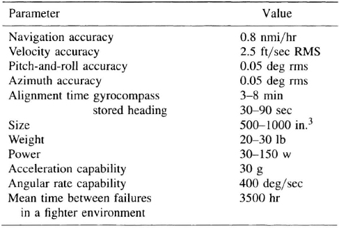
Mechanization In a strapdown navigator, gyroscopes and accelerometers are rigidly mounted to a sensor assembly that is usually mounted to the vehicle on a set of shock mounts. The gyroscopes track the rotation of the body and drive an algorithm that calculates the orientation of the vehicle. The accelerometer outputs are transformed to the navigation axes by the computed rotation matrix. This leads to the analytic platform, a computed set of stabilized axes, which are analogous to the stable element axes in a gimballed system. The transformed accelerometer outputs are integrated to velocity in the analytic platform coordinate system. In a strapdown system the gyroscopes do not act as null-sensors (as in gimballed units) but sense the inertial angular rate of the vehicle. An extremely high dynamic range (0.005 deg/hr to 400 deg/sec or more) is required in many applications. Further, the calculation of system orientation and the transformation of accelerations require complex computations. Strapdown navigation systems have been made possible by optical gyroscopes and high-throughput computers [44, 45], Since the mid-1980s, navigation performance has been similar to the best gimballed systems. Strapdown units offer additional advantages such as extended bandwidth, reduced mechanical complexity, wide temperature operation, and improved reliability. Table 7.1 shows typical characteristics of a strapdown inertial navigation unit. The error propagation of a strapdown navigator follows the same laws as gimballed navigators, but errors depend more heavily on trajectory, since the instrument orientation varies as the aircraft maneuvers.

Strapdown Computations The purposes of these computations are (1) to calculate the vehicle's attitude relative to the navigation coordinates using the gyro measurements, (2) to transform the accelerometer measurements from vehicle axes into navigation coordinates, and (3) to perform the dead-reckoning computations of Equation 2.5.

TABLE 7.1 Typical inertial navigator specification (1996)

Attitude Integration In three dimensions, it is not possible to add rotation angles. The readers may convince themselves of this point by manipulating a three-dimensional object with labeled x-, y-, and z-axes. For example, as illustrated in Figure 7.17, a 90-deg rotation about the x-axis followed by a 90-deg rotation about the z-axis yields a different final orientation as compared to a 90-deg rotation about the z-axis followed by a 90-deg rotation about the x-axis. This example involving large angles illustrates the principle of noncommutativity discussed in many references [4, 16]. Noncommutativity also applies in the case of small angles. Attitude computations must therefore take into account the properties of rotations.

In three dimensions rotations may be described by three or more parameters. Three-parameter definitions include the Euler angles, which specify three rotation angles taken in a specific order (thereby emulating a gimbal set). Unfortunately, the Euler angles suffer from singularities (as do all three parameter systems) and extreme nonlinearity and are ill-suited for attitude integration. They are. however, commonly used as attitude readout parameters. The rotation vector is another three-parameter description of rotation. Such a vector specifies an instantaneous axis of rotation and the angle of rotation about this axis (any orientation can be transformed to any other by a single-axis rotation). The rotation vector is a useful concept for small angles but is difficult to manipulate for large rotations.

The most common means of describing rotation in strapdown systems employ more than the minimum three parameters [37]. A calculation using direction cosines [21] was briefly in use for slowly rotating vehicles in the 1960s. In the late 1960s, quaternions supplanted the direction cosines, and, in the early 1970s, preprocessing of the gyro outputs was introduced to speed up the computations.

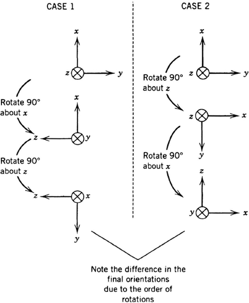
Figure 7.17 Example of noncommutativity of rotations.

Direction Cosine Formulation A direction-cosine matrix is mathematically well behaved and suited for integration. Vectors are easily transformed using these matrices.

Let the vehicle's coordinate frame (the body frame) be denoted by B, and the navigation coordinate frame by N. The direction cosine matrix transforming from the body coordinates to the navigation coordinates is . The exact relationship between and the instantaneous angular rate is

where is the instantaneous angular rate vector of the body frame with respect to the navigation frame as measured in body coordinates, is the same angular-rate vector, resolved into navigation coordinates, and the [ω] matrix is:

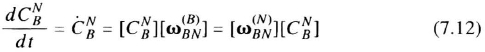
The solution to the differential equation (7.12) is updated at specific intervals determined by the computer's workload. Thus, strapdown gyros must be “rate-integrating gyros” that measure the integral of the component of angular velocity along their input axes (sometimes called “incremental angles” Δθ_i) during the computing interval. From the Δθ_i, the computer calculates the aircraft's attitude change during the interval. The Δθ outputs of the integrating gyros are numerically scaled as angles though they do not represent geometric angles because they do not form a true vector; consecutive Δθ are neither additive nor commutative. The smaller the angle, the more closely Δθ approximates a vector and represents the change in attitude. Note that a rate gyro, that samples the instantaneous rate sometime during the computing interval, would introduce large attitude errors because the rates change during the iteration interval.

To a first approximation,

This is a method of calculating the nine elements of the direction cosine matrix C at each read-time from the set of three gyro measurements. It is practical only in the slowest-rotating applications such as some land vehicles and spacecraft because of the following problems:

1. The C matrix will gradually become nonorthonormal and nonorthogonal unless explicitly corrected. Orthonormality requires that the sum of the squares of any row or column equal unity, and orthogonality requires that the dot products of any two rows or columns equal zero. Mathematically,

   

   where δ_ij is the Kronecker delta (δ_ij = 1 for i = j, δ_ij = 0 for i ≠ j).

2. There are nine simultaneous equations to be propagated at each gyro-read interval.
3. Rate-integrating gyros prevent the loss of angular information in the presence of angular acceleration during the gyro-read interval. However, a change in the direction of the angular rate vector during the interval leads to noncommutativity or coning errors, which render Equation 7.14 inaccurate.

Quaternion Formulation The first two problems described above are avoided through the use of quaternions. A quaternion is a four-element entity consisting of a scalar part λ and a vector part ρ with the following representation:

It defines the instantaneous axis of rotation. The product of two quaternions is defined as

For a rotation quaternion, the norm is unity (given by λ² + ρ · ρ = 1). Thus, there is a single normalization constraint (the sum of the squares of the four elements must be equal to unity). A rotation quaternion may be expressed as

where 1_ϕ sin (ϕ/2) is the vector part ρ and cos ϕ/2 is the scalar part λ. Thus, any rotation can be expressed as a single rotation about an inclined axis. In this case, 1_ϕ is the unit vector along the inclined axis of rotation and ϕ is the angle of rotation about that axis.

The quaternion inverse is given by

The differential equation for a quaternion is

where ω is the instantaneous angular rate vector. The exact solution to equation (7.19) is given by

This equation must be solved using the incremental angles measured by the gyroscopes. To a first approximation, the vector change in angle is related to the angular rate vector sensed in the form shown below:

A better approximation is needed in aircraft systems as discussed in the next paragraph. The quaternion update algorithm is executed at a rate (typically 50 to 500 times per second) such that the magnitude of the Δϕ vector will remain small (0.01 sec at 50 deg/sec = 0.5 deg). In this case, a second-order expansion is used for cos Δϕ/2 ≈ 1 − ((Δϕ)²/8) and for sin (Δϕ/2)/(Δϕ/2) ≈ 1 − (Δϕ)²/24. Quaternion integration algorithms usually make use of the normalization constraint to control error growth in the computations. The sum of the squares of the quaternion elements are subtracted from unity to yield the normalization error.

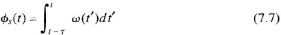
Coning Errors Coning refers to a motion in which the axis of rotation is itself moving in space. In this type of motion, the axes of the body trace a cone in space. Reference [16] demonstrates that a gyroscope whose input axis describes a cone will sense an average angular rate equal to the solid angle swept per unit time. However, there is, in fact, no net rotation taking place about that axis. In the other two axes perpendicular to the coning axis, the actual motion may be described as “oscillatory signals in phase-quadrature.” Because the attitude integration in a strapdown system takes place at a finite iteration frequency, the oscillatory components will not be faithfully reproduced (particularly if the coning frequency approaches or exceeds the iteration frequency), and a net error will be generated. This error is attributed to the approximation Δϕ ≈ Δθ in Equation 7.21. The net coning error depends on the coning frequency f_c and the iteration interval Δt and is proportional to the coning rate Ω_c:

For a circular cone of angle α and frequency f_c,

The apparent drift rate increases with the frequency and amplitude of the coning motion. Coning errors may be reduced by raising the quaternion iteration frequency but this is costly in terms of computer throughput [37]. Instead, an algorithm preprocesses the gyro data at a higher rate than the quaternion integration to improve the approximation in Equation 7.21 in order to follow the actual motion of the rotation axis closely. The algorithm computes an average rotation over the slower quaternion update interval. The preprocessing algorithms are sometimes called coning algorithms [28, 37, 46]. An example of a coning algorithm is given below.

Every “fast” preprocessing cycle

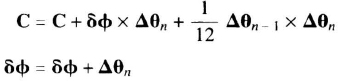
Every “slow” quaternion update cycle

where

n	is the fast iteration counter
C	is the vector coning correction
Δθn	is the three axis integrated rate over the nth fast cycle
δϕ	is the resettable integration of Δθ
Δϕ	is the rotation vector used to propagate the quaternion over one “slow” cycle

At the end of the “slow” cycle Δϕ updates the quaternion as in Equation 7.20. Typically, the preprocessing algorithm executes up to 2000 times per second, while the quaternion algorithm executes 50 to 250 times per second.

Direction Cosine Formation A direction cosine matrix may be calculated exactly from a rotation quaternion. If the quaternion is properly normalized, the resulting direction cosine matrix will always be orthogonal and orthonormal:

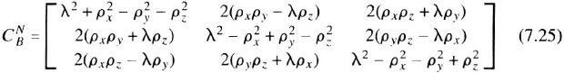
Euler angles may be extracted from this matrix as discussed in Section 7.5.1. In a quaternion mechanization, the Euler parameters serve strictly as system outputs for attitude (e.g., to show roll and pitch).

Incremental Velocity Transformation Accelerations sensed in the body frame are transformed through the body-to-navigation direction-cosine matrix in order to compute acceleration in a stabilized coordinate system. However, because this transformation cannot be performed on a continuous basis, the accelerometer outputs are integrated in the body frame to form incremental velocities (ΔV) which are then transformed to the navigation frame:

(Between transformations)

(Transformation)

The use of incremental velocities instead of instantaneous acceleration is important to preserve the correct velocity in the presence of changing acceleration during a sampling interval. The approximation in Equation 7.26 can lead to sculling errors, as discussed on page 359.

Quaternion Navigation Updates The gyroscope outputs update the quaternion as given in Equation 7.20. However, gyroscopes measure rotation relative to inertial space, while navigation is generally performed in Earth-fixed, local-level coordinates, as discussed in Section 7.5. Thus, the attitude quaternion must be modified to account for the rotation of the Earth and the travel of the vehicle around the Earth. The combination of these two terms describes the rotation of the locally level plane with respect to inertial space. A quaternion torquing algorithm (analogous to gimbal torquing) is used in addition to the body update algorithm to permit tracking of attitude with respect to the locally level plane. The algorithm that employs torquing rate commands (also known as tilt corrections) is given below:

where

with

where ω_L is the torquing rate vector. The rotation rate of the navigation frame is usually less than 50 deg/hr. Thus, the iteration frequency of the navigation updates can be substantially lower than that of the body updates. Further, due to the very small angles involved (Earth rate over a 10-Hz interval represents only 7.5 µrad of angle change), a first-order expansion of the trigonometric functions

is usually all that is needed in Equation 7.28.

Packaging The gyros and accelerometers are rigidly mounted on a block with temperature sensors. The block is usually shock-mounted to the vehicle to control the bandwidth of the motion sensed at the instruments [33]. Shock-mounting limits vibration rectification errors within the instruments themselves (accelerometers. in particular). In choosing the natural frequency of the isolation mount, trade-offs must be made between bandwidth, navigation accuracy, and computational throughput. In all cases, the isolation system must be designed to avoid vibration-induced coning and sculling errors. If the strapdown instruments are used for flight control, tight coupling to the vehicle (e.g., high bandwidth) is desirable, though it increases navigational errors.

In the 1970s, some early strapdown blocks were mounted on a gimbal-like turntable for preflight calibration and employed heaters for thermal stabilization. Optical gyroscopes have eliminated the need for turntables and heaters in the majority of applications. A typical strapdown sensor assembly is shown in Figure 7.18.

Figure 7.18 Typical strapdown inertial navigator or RLG sensor assembly (courtesy, Honeywell Inc.).

For fault tolerance, blocks may contain more than the minimum of three single-axis gyroscopes and accelerometers. With four of each, fail-safe operation is obtained allowing the detection but not necessarily the isolation of a single failure. Isolation is the process of determining which instrument failed and changing the algorithm to use the remaining instruments for navigation. With six gyroscopes and six accelerometers, detection and isolation of up to two failures of each type of sensor is possible. Some systems have been constructed with six RLGs and accelerometers on a single isolated sensor assembly. They have been applied to space-launch vehicles. However, the added complexity of maintaining six redundant channels has made them costly and bulky, so they are not widely used. Aircraft operators prefer redundant IMUs, each having three single-axis gyroscopes and accelerometers.

Calibration Instruments must be calibrated at the factory and compensated during flight for best performance. In the factory, systems are mounted on rate tables, and specific motions are executed to excite various error sources. For example, rotation about a given axis will excite gyro scale factor and misalignment errors. Tipping an accelerometer into gravity will excite accelerometer scale factor and misalignment errors. In certain calibration procedures, a large number of measurements are taken, and the data are reduced in a least-squares program to fit the anticipated error model [5]. Reference [34] presents an attractive method for isolating individual error sources in minimum time. Often, the calibration steps are repeated over a wide temperature range in order to generate thermal models for the instrument parameters.

Most strapdown systems do not require re-calibration since optical gyroscopes exhibit excellent long-term stability and since in-flight Kalman filters recalibrate the instruments during operation. Curve fits of the following parameters are made in the factory as a function of temperature and the model coefficients are stored in nonvolatile calibration memory:

• Gyro bias
• Gyro scale factor
• Gyro misalignment
• Accelerometer bias
• Accelerometer scale factor
• Accelerometer misalignment

For mechanical gyros, mass unbalance is also calibrated.

In flight, the strapdown sensors (generally not temperature controlled) are compensated based on measured temperature, using the models stored at the factory. The navigation filter is able to calculate residual instrument errors if an independent source of velocity or position information (e.g., GPS, Doppler radar, or star-tracker) is available. A Kalman filter (Chapter 3) often fine-tunes gyro and accelerometer biases in flight. More complex Kalman filters may also calibrate scale factor and misalignment states.

Size, Weight, and Performance Instrument error models are given in Section 7.3 (for accelerometers in 7.3.1, for optical gyroscopes in 7.3.3, for mechanical gyroscopes in 7.3.4). Strapdown systems have added errors due to trajectory, angular acceleration, and computing cycle time.

Coning Errors In military aircraft, large coning rates are generated in maneuvers known as S turns. Large roll and azimuth rotations occur 90 deg out of phase, leading to a large coning rate about the pitch axis. If ±45-deg turns occur four times per minute, a coning rate of 25,000 deg/hr will be generated. The observed system drift will depend on the effectiveness of the coning and quaternion algorithms [28, 37, 46] as well as on the scale factor and misalignment accuracies. Errors as small as a few parts per million or a few microradians are significant.

Sculling Errors If the acceleration vector were measured, transformed to stabilized navigation coordinates continuously, and integrated to velocity, no error would be incurred. The computed ΔV would be

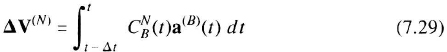
However, the accelerometers integrate acceleration in the body frame at discrete intervals. This yields the approximation of Equations 7.26 and 7.27.

In the presence of combined rotation and acceleration known as sculling, this approximation can lead to errors referred to as sculling errors. Figure 7.19 illustrates sculling and indicates how errors are generated. In the presence of a rotation synchronous with an oscillating acceleration, an average acceleration is erroneously computed. For most mechanizations, the residual acceleration error for small angular motions may be expressed as

where a₀ is the amplitude of the oscillatory acceleration and θ₀ is the amplitude of the oscillatory angular motion in radians. Sculling error is usually expressed in µg.

To avoid large sculling errors, it is necessary to execute the velocity transformation at least four times faster than the anticipated frequencies of vibration. It is also possible to use a high-iteration-rate sculling algorithm. It computes the cross-product between the gyro data and the accelerometer data to improve the approximation in Equation 7.27. It is important to use wide-band-width accelerometers in order to reconstruct the oscillatory information.

Size-Effect Errors It is impossible to co-locate the three accelerometers. As a result, each accelerometer senses acceleration at a slightly different point in space (typical separations are on the order of a few centimeters). In the presence of angular motion, each of the accelerometers will sense centripetal and/or tangential acceleration. The set of three accelerometer outputs will not be consistent due to their different physical locations. The result is a size-effect (lever-arm) error. The size-effect error rectifies with a magnitude proportional to the distance between accelerometer centers and the square of the angular rate. Size-effect errors do not occur in gimballed systems, since the accelerometers are isolated from angular motion.

Figure 7.19 Illustration of sculling motion.

Size-effect errors can be excited with low-frequency rocking motion. For example, if a system is rotated ±45 deg with a period of 4 sec and an accelerometer lever arm of 2 cm, the size-effect is:

This error is easily corrected in the computer.

7.4.2 Gimballed Platform

The purposes of a stable platform are the following:

1. To orient the accelerometers in a definite coordinate frame relative to the Earth or inertial space, despite angular motions of the vehicle.
2. To provide a convenient readout of vehicle attitude by reading each of the gimbal angles separately, thereby yielding convenient Euler angle outputs.
3. To protect the accelerometers and stabilization gyros from large angular motions of the vehicle, which would cause incorrect operation.
4. To protect the instruments from vibration, temperature, and magnetic environments.

Gimbal Order A schematic diagram of a four-gimbal stable platform is shown in Figure 7.2. Though four-axis platforms were universally used on aircraft, the three-axis platform will be discussed first for clarity. A three-axis platform is formed by holding the inner-roll angle (B angle) of the four-gimbal platform rigidly at zero. The vehicle is free to rotate about the roll, pitch, or yaw axes without disturbing the stable element.

Any gimbal order can be chosen, subject to limitations imposed by the mission. The innermost and outermost gimbal axes have potentially unlimited freedom, whereas the middle axis (pitch in Figure 7.2) is limited to approximately ±70 deg. The condition in which the middle-gimbal angle approaches 90 deg is called gimbal lock. In this condition, the innermost and outermost axes coincide, thus depriving the platform of one of its degrees of freedom. All-attitude operation can be achieved with a four-axis platform as described on page 363.

Stabilization In some simple systems, the orientation of the stable element is maintained by brute-force gyro stabilization, relying on the moments of inertia of the stable element and the angular momentum of the gyros to reduce the precession caused by small friction torques. Brute-force stabilization is used only on platforms designed for a few seconds of flight, where the precession rate of the platform (friction torque ÷ H) is acceptably low.

In most cases, servo stabilization is needed in order to maintain the orientation of the stable element (Figure 7.2). The error detectors, which provide inputs to the stabilization servos, are typically precision TDF gyroscopes. Their outputs are resolved and used to drive the gimbal servos.

The ability of the stable element to remain nonrotating relative to a space or Earth coordinate frame depends on the following factors:

1. Drift rate of the reference gyros
2. Accuracy of the gyro torquers
3. Angular motion of the vehicle (vehicle motion isolation)
4. Orthogonality of components on the platform

Gyro errors are discussed in Section 7.3.4. Base-motion isolation and cross-coupling are measured by nine ratios (ω_pi/ω_bj). Each of these ratios measures the angular velocity of the stable element about the x_ith-axis (ω_pi) in response to the angular velocity of the vehicle about the y_jth-axis (ω_bj). These ratios serve as a measure of platform performance, since they indicate how well the platform isolates the instruments from vehicle motion. The nine ratios provide measures of in-axis as well as cross-axis isolation as a function of frequency.

The degree of base-motion isolation is largely determined by the servo characteristics. For a single-axis platform using TDF gyros for stabilization, the platform response has the form

where T_i are functions of the gimbal drives, moments of inertia, and of the damping. A more exact analysis would include the characteristic time of the gyro and the intergimbal coupling.

Another parameter of importance is the platform's response to gyro-torquing signals (e.g., those commanding the platform to remain locally level and north oriented). The torque commands change slowly, even when the vehicle executes a high-speed turn. As a result, there is seldom a problem of attenuation of command signals in the servos. The design of gimbal servos is discussed in detail in [40, 41] and Chapter 3 of [7].

Mechanical Design From the mechanical designer's viewpoint, the platform serves the following three functions:

1. Vibration control. The gimbal structure should attenuate vibration (externally-induced and self-excited due to spinning gyros and other gimbal-mounted components), thus allowing the gyros and accelerometers to operate in a benign environment. The gimbals should exhibit no undue resonances and should not have vibration characteristics that are strong functions of gimbal angle. Attempts have been made to build gimbals of a laminated material that has good dimensional stability and can detune resonance peaks. Shock mounts are usually needed to supplement the gimbal's attenuation characteristics.
2. Temperature control. Most mechanical gyros and accelerometers must be held within a degree or less of their desired operating temperature (and temperature gradient) in order to maintain full accuracy. As a result, the gimbal system and housing must provide for suitable conduction and convection (usually using cooling air) of heat from gyros, accelerometers, motors, and gimbal-mounted electronics. An air-to-fluid heat exchanger or Peltier-effect refrigerator can prevent contaminated cabin-cooling air from entering the platform cavity. Temperature control of the stable element must be independent of changes in the gimbal angles. This requires ingenuity in the method of circulating coolant within the platform cavity. Rapid warmup may impose stringent requirements for preventing large temperature gradients in the stable element. The measurement of gyro temperature and the computation of compensations eases the problem.
3. Magnetic field control. Gyros and accelerometers are often magnetically sensitive. Each instrument so affected is usually separately shielded. However, care must be taken to prevent large externally (cables, radars) or internally (direct-drive gimbal torque motors) generated fields from affecting the instruments.

Misalignments between instruments cause navigation errors, as discussed in [25]. For example, a gyro-to-gyro misalignment β causes an apparent drift rate βω_m, where ω_m, is the platform precession rate. Orthogonality errors can be corrected mechanically during assembly, or they can be computer-compensated in the outputs of the instruments. Aircraft platforms are typically orthogonalized within minutes of arc. It is important that the platform be designed so that the orthogonality angles do not change in the presence of vibration and repeated thermal cycling.

Four-Axis Platform A four-axis, all-attitude platform is shown schematically in Figure 7.2. Its inner three gimbals are identical to those of a three-axis platform. In normal flight, B is servoed to zero; A, C, D are the degrees of freedom. At near-vertical aircraft attitudes (C ≈ 90deg), A = 0, and B, C, D are the degrees of freedom. Much ingenuity has been exercised in designing control circuits to execute the transition from A, C, D freedom (B = 0) to B, C, D freedom (A = 0).

The four-gimbal platform trades the gimbal-lock problem for the “flip” problem exhibited when the C-axis approaches 90 deg and D must flip through an angle of 180 deg. Whereas a three-gimbal platform would tumble in the gimbal-lock position, the four-gimbal platform does not, as long as the gimbal servos are fast enough to prevent the gyros from hitting their stops during the flip maneuver. Electric power and servo signals must be carried from gimbal to gimbal. Axes of limited freedom can be supplied with coiled wires. Other axes require slip rings. Figure 7.20 shows a four-axis aircraft navigation platform.

Figure 7.20 Typical aircraft inertial platform (courtesy, Litton Systems).

7.4.3 Inertial Specifications

A typical performance specification for an inertial system contains the following:

1. Size and weight.
2. Cooling and/or heating requirements.
3. Power consumption during warm-up and cruise. Increased servo power required during maneuvers (platforms only). Power regulation (voltage and frequency) and susceptibility to transients and momentary dropouts.
4. Maximum rates and accelerations along and around each axis.
5. Vibration specifications for survivability and for meeting specified navigation performance.
6. Shock-mount returnability and maximum angular deflection.
7. Reliability including MTBF (mean time between failure) and recalibration interval (if applicable).
8. Self-test capability and equipment integrity.

Inertial systems for civil use are packaged in accordance with ARINC specifications [60]. Military systems must conform to the applicable Department of Defense standards and specifications such as [62]. The equipment used to test platforms or strapdown systems include the rate table (two- or three-axis) which applies angular rates about different axes and the vibration table which supplies oscillatory motion to the system. Rate tables are sometimes used in Scorsby mode whereby a sine motion on one axis is simultaneously applied with a cosine on the other. This test induces a coning rate in the instrument package. Rate table and vibration tests are also performed over temperature using thermal chambers. For some applications, centrifuges and rocket-propelled sleds may be used to test system parameters and sensitivities. Tests of individual instruments are discussed in Sections 7.3.4 and 7.4.1.

7.5 MECHANIZATION EQUATIONS

The mechanization equations calculate velocity and position from the outputs of the horizontal accelerometers in a platform or from the transformed accelerations in a strapdown system. This section discusses those portions of the mechanization equations that calculate velocity of the aircraft relative to the ground. Section 2.4 discusses the navigation computation equations that convert ground velocity into position.

7.5.1 Coordinate Frames

Several coordinate frames must be defined for the purposes of mechanizing an inertial navigator, Section 2.3. Figure 7.21a shows the I coordinate frame (ECI) with x-, y-, and z-axes centered at the mass center of the Earth and nonrotating in inertial space (nonrotating relative to the stars). Such a coordinate frame can be regarded as inertial if the measurement accuracy is not more precise than 5 × 10⁻⁵ deg/hr and 2 × 10⁻⁷ g [26], The E coordinate frame has its origin at the mass center of the Earth and is fixed to the Earth with its z-axis along the spin axis of the Earth. This frame is also known as the Earth-centered, Earth-fixed (ECEF) frame. It rotates at Ω = 15.04107 deg/hr relative to the ECI frame, to an accuracy of 5 × 10⁻⁵ deg/hr [26].

The geographic coordinates in which the vehicle position is calculated are labelled G. Figure 7.21a shows the latitude-longitude coordinate frame. x^(G) points level and east; y^(G) points level and north; z^(G) points vertically up (along the g vector; see Section 2.2).

The navigation (or platform) coordinates N lie along the orthogonal accelerometer input axes in the case of a gimballed platform. In a strapdown system the N coordinates are the axes of the analytic platform defined by the coordinate transformation matrix or quaternion. As discussed in Section 7.4.1, these axes represent a set of orthogonal accelerometers whose x and y axes are level and whose y-axis makes an angle α west of true north (see Figure 7.23). The use of an analytic platform renders the transformed strapdown acceleration outputs equivalent to the outputs of mechanically stabilized accelerometers. All navigation mechanization equations then become common to both forms of systems. The α angle is known as the wander azimuth and its use facilitates navigation in the polar regions. The navigation frame is related to the Earth frame by the following matrix:

Figure 7.21a Navigation coordinate frame definition.

where

Φ	is the latitude
λ	is the longitude
α	is the wander azimuth

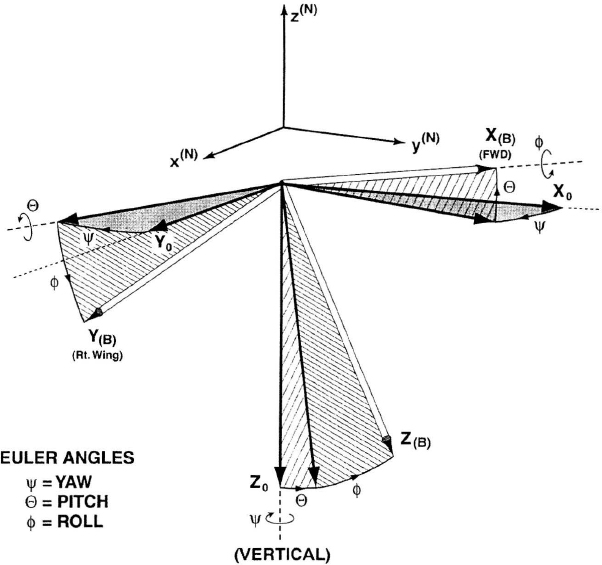
Figure 7.21b Euler angles: X₀, Y₀, Z₀ reference axes at ψ = θ = ϕ = 0. X_B, Y_B, Z_B vehicle body axes.

Ci	are cos(i)
Si	are sin(i)

In a strapdown system an additional coordinate transformation relates the body frame (illustrated in Figure 7.21b) to the navigation frame:

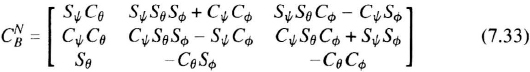
where

ψ	is yaw
θ	is pitch
ϕ	is roll

7.5.2 Horizontal Mechanization

The differential equations that must be solved for navigation are given by

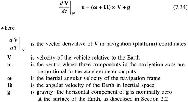
The solution of these equations lead to the computation of ground speed using the mechanization illustrated in Figure 7.22 where the navigation components of V are calculated from the accelerometer outputs u. The Coriolis correction (generated by velocity in the presence of platform angular velocity) is given by

The navigation frame must rotate at ω_i in inertial space; hence, ω_i, “torques” the analytic platform as discussed in Section 7.4.1 for strapdown systems or torques the mechanical platform as discussed in Section 7.4.2 for gimballed systems. The forms of ω_i and Ω_i depend on the choice of navigation coordinates, some of which are noted below:

1. Locally level, north pointing, x^(N) along x^(G), y^(N) along y^(G), z^(N) along z^(G)):

   

   

   Figure 7.22 Mechanization of an inertial navigator.

   where

   Φ	is the latitude of vehicle
   λ	is the rate of change of vehicle longitude
   Vx	is east velocity
   Vy	is north velocity
   RM	is the radius of curvature of the Earth in the meridional plane, Equation 2.2
   RP	is the radius of curvature of the Earth in the vertical east–west plane, Equation 2.3

2. Locally level, wander azimuth [27][42]; x^(N) and y^(N) are in a level plane, with y^(N) at an angle α from y^(G); z^(N) lies along z^(G) (Figure 7.23).

   

   Figure 7.23 Plan view of a level platform at an azimuth α.

   

   

   where V_x and V_y are the level components of the velocity vector in the navigation coordinates and α is the azimuth of the y^(N)-axis relative to north (Figure 7.23).

3. Tangent plane; y^(N) north at point of tangency (Figure 2.3):

   

   where Φ₀ is the latitude at the point of tangency, usually the takeoff point.

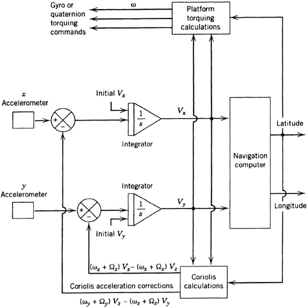
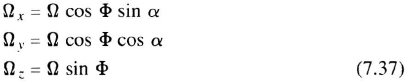
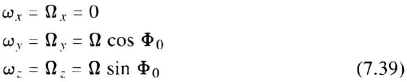
The first coordinate frame offers the advantages of simplicity at low latitudes, the readout of familiar latitude-longitude coordinates from the computer, and the measurement of vehicle heading directly from the direction cosine matrix in a strapdown system or from the platform azimuth angle in a gimballed system. Unfortunately, this mechanization exhibits polar singularities at high latitudes.

The second coordinate frame introduces the complexity of an extra coordinate, the wander angle α, in exchange for the following advantages:

1. Operation at all latitudes, with the correct choice of mechanizing .
2. Omission of the azimuth torquing by setting ω_z = 0 (free azimuth).
3. In gimballed platforms, some improvement in navigation performance can be achieved by continuous azimuth rotation at a constant rate . The instrument axes point in various directions thus tending to cancel the effect of their drift. In one platform [6] was 50 times Earth rate, so that instrument drifts whose correlation time was greater than one-half hour tended to be smoothed. The azimuth rotation can be reversed periodically to reduce the effects of an azimuth-gyro torquer error. Such performance improvements cannot be achieved in strapdown systems because the instruments remain fixed to the body.

Wander-azimuth systems do not read vehicle heading directly from the direction cosine matrix or the platform azimuth gimbal. The vehicle's heading relative to north is platform-indicated azimuth minus α. Heading becomes indeterminate at the poles. The majority of inertial navigation systems implement a wander azimuth, since the benefits outweigh the additional computational complexity involved. As an illustration of a typical mechanization, consider the wander-azimuth system of Equations 7.37 and 7.38:

1. Integration of Equations 7.34 yields V from the accelerometer outputs.
2. The torquing signals are calculated from V according to Equations 7.37 and 7.38 and the azimuth condition . Notice that vehicle latitude and the wander angle are required for this calculation. Longitude and azimuth exhibit polar singularities and therefore should not be used as fundamental variables for worldwide operation. Instead, the direction cosines C_ij of the N axes relative to the E axes are introduced (Equation 7.32). These parameters are mathematically well behaved at all latitudes even when longitude and azimuth are not. The direction cosines obey the differential equations

   

   and latitude-longitude coordinates are calculated from

   

   α is calculated only when it is convergent:

   

3. The wander angle α can be constructed in many ways. Clearly, if α itself had to be calculated as part of the position-velocity mechanization, the system would not be convergent over the poles. However, , defined as ω_z − Ω sin Φ, can always be calculated in a convergent manner. The wander angle α is not used explicitly in the navigation solution. The wander azimuth may be extracted for readout purposes using Equation 7.42. Wander-azimuth mechanizations include, as special cases, all locally level systems. For example, in a north-pointing system, α is constrained to be zero.
4. In early navigation systems, where computational throughput was at a premium, updating of the direction cosines was performed at a low iteration rate (a few times per second). In 1996, inertial systems included sufficient computer power to perform the updates 50 or more times per second. Direction-cosine algorithms generally have employed 32 bit-integer word length, but microprocessors in the 1990s used floating-point instructions to enhance accuracy.

An insight into the nature of the inertial mechanization can be obtained by considering the steady-state situation in level flight.

1. The outputs of the level accelerometers are virtually zero, except for the Coriolis acceleration, and accelerations due to air turbulence and equipment vibration. Barring inadvertent rectification within the accelerometers, vibration-like outputs do not indicate any net position change, no matter where in the aircraft the instruments are located.
2. The dV_i/dt in the computer are zero, since the computer-calculated gravity vector g and Coriolis correction (ω + Ω) × V just cancel the gravity and Coriolis accelerations measured by the accelerometers.
3. The velocity registers do not change.
4. The computed position changes slowly as the vehicle moves over the Earth.
5. The torquing signals are nearly constant, changing slowly as the latitude and heading of the vehicle change.

Section 2.7 shows how inertially derived position is used for steering. Locally level mechanizations are desirable in terrestrial navigation systems for the following reasons:

1. In a gimballed, north-pointing system, roll, pitch, and azimuth are directly available as gimbal angles. In a strapdown system, they are mathematically extracted from the quaternion/direction cosine representation. For wander-azimuth mechanizations, the platform (mechanical or analytic) yaw angle minus the computer-calculated α equals true azimuth.
2. No gravity corrections are needed in the horizontal accelerometer channels. A small component of gravity is measured by the horizontal accelerometer channels when they are tilted from the locally level plane or when gravity anomalies exist (see Section 2.2).
3. For a gimballed platform, the gyros require accurate mass balance in only one orientation, since horizontal acceleration is intermittent.

In some instances (particularly space applications), inertial systems may use nonlocally level navigation frames. Reference [58] discusses an Earth-fixed cartesian mechanization.

In pure inertial systems without external updates, constant instrument errors tend to cause oscillatory position, velocity, tilt, and azimuth errors as discussed in Section 7.6. Stationary noise in the instruments tends to cause errors that grow with the square root of time. For aircraft systems that operate for only a few Schuler periods (multiples of 84.4 minutes), a pure inertial system is often adequate. Growth of errors can be reduced by periodic position, velocity, or azimuth updates (e.g., radio or celestial). Reference [13] discusses the effects of the frequency of fixing on error propagation. Chapter 3 discusses multisensor navigation systems in which frequent external fixes are analytically combined with inertial measurements.

7.5.3 Vertical Mechanization

It might appear that altitude could be calculated by double integration of the measured vertical acceleration. Unfortunately, such a mechanization would be unstable, as will now be shown. Assume a constant-velocity flight at a speed that is negligible compared with orbital speed. Let:

Then

Expanding and letting Δh = h_c − h_a,

whose solution is

For the first few seconds of flight:

An initial altitude error (Δh₀) or altitude-rate error or an accelerometer error (A₀) will lead to an exponential growth in computed altitude (doubling in the first 78 minutes), thus making the indicated altitude and altitude-rate useless after the first few minutes. The instability of the vertical channel will result, no matter how carefully the vertical component of gravity is mechanized as a function of computed altitude.

On the other hand, a barometric altimeter is very stable for long periods of time but suffers from a noisy output and a long time lag (due to aerodynamic noise and the dynamics of air flowing through tubes, ports, and orifices; see Section 8.2). As a result, instantaneous readings of altitude and altitude-rate are impossible. The best features of inertial and barometric altimeters can be combined in a baroinertial altimeter shown in Figure 7.24. By comparing barometric altitude with inertial altitude and feeding back through suitable filters, the indicated altitude can have (1) the long-term stability of the barometric altimeter, (2) a frequency response that is much faster than that of a pure barometric altimeter but that attenuates barometric noise, and (3) relative insensitivity to low-frequency accelerometer errors.

Figure 7.24 Mechanization of a stable baro-inertial altimeter.

The transfer function shown in Figure 7.24 (where G₁ and G₂ are constant gains and the system is of second order) demonstrates that in a baro-inertial altimeter, a constant accelerometer error A₀ causes an altitude error or approximately where ω_N is the natural frequency of the altimeter loop. A bias change of 1 mg causes only a few inches of altitude error for a one-minute natural period. As a result, the Coriolis correction can usually be omitted and vertical gravity can be computed as a constant, independently of altitude and latitude. Nonetheless, most modern inertial navigation systems implement a more complete gravity model. This permits more accurate vertical channel operation particularly at high altitudes. Baro-inertial altitude and altitude-rate are used in weapon delivery computers and in the calculation of flight path angle, γ

Further information regarding standard baro-inertial loops may be found in reference [3], If the statistical properties of the accelerometer and altimeter noise are known, an optimum filter (Chapter 3) can be designed to give the best estimate of altitude and altitude rate. More sophisticated mechanizations may include estimates of the accelerometer bias and barometer scale factor [2].

7.6 ERROR ANALYSIS

7.6.1 Purpose

After mechanizing an inertial navigation system, the designer must investigate the propagation of errors in the proposed system, based on mathematical analysis and on the results of past tests. The error analysis establishes the maximum permissible component tolerances; to simplify the mechanization equations (and thus the computer complexity) when advantageous; and to predict compliance with the position, velocity, attitude, and azimuth specifications established by the user.

The sources of error that should be considered in performing the analysis depend on the system design, the components used, and the required accuracy of the navigation system. Some typical sources of error are enumerated below (instrument errors are discussed in more detail in Section 7.3).

1. Gyro drift errors caused by temperature variation, acceleration, magnetic fields, and vibration.
2. Gyro scale factor errors including nonlinearity and asymmetry.
3. Accelerometer bias errors caused by variations in temperature or by rectification of vibration inputs. Accelerometer resonances and dynamic response are important considerations.
4. Accelerometer scale factor errors including nonlinearity and asymmetry.
5. Sensor assembly errors such as nonorthogonality of the gyro and accelerometer input axes, transmission of vibration inputs through the shock mounts, and thermal gradients that affect instrument performance and alignment.
6. Computational errors due to roundoff, truncation, readout accuracy, as well as approximations inherent in the algorithms. Detailed evaluation of computational error propagation often requires a bit-by-bit simulation.
7. Initial condition errors (position, velocity, tilt, and azimuth) must be considered as they propagate with time.

7.6.2 Simulation

Error analysis is performed by assuming a flight path and processing the resulting acceleration and angular-rate profile in a mathematical model of the inertial system and computer. The indicated positions and velocities are compared to the assumed flight path, and the error histories are recorded. Azimuth and tilt errors can similarly be derived. Analyses are done either with fixed instrument errors or with statistically distributed errors in a large number of runs (Monte Carlo simulations).

7.6.3 Error Propagation

A complete simulation assesses overall system performance for particular trajectories. It yields a time-varying covariance matrix (Chapter 3) that quantifies the growth of errors and the correlations among errors. However, to understand the physical causes of errors and to troubleshoot systems, a simplified closed-form analysis is invaluable. For simple flight profiles (e.g., straight legs, 90-deg-turns), deterministic initial-condition and instrument errors are readily propagated with time, using analytic approximations. The solution is complicated by the correlation that exists between in-flight instrument errors and the initial conditions. In gimballed systems, some instrument errors during alignment tend to cancel the same instrument errors incurred in flight. However, in strapdown systems, the instrument axes rotate with respect to the analytic platform axes and error cancellation may not occur. Therefore, the propagation of errors is far more dependent upon the trajectories in strapdown systems.

For closed-form analysis, the mechanization equations can be linearized for a vehicle moving at low speed (relative to the surface speed of the rotation of the Earth). The result is that undamped oscillations are present in the position, velocity, tilt, and azimuth errors. The frequencies of these oscillations are (1) Ω, Earth rate; (2) , the Schuler frequency (84.4-minute period); and (3) beats between ω_s + Ω sin Φ and ω_s − Ω sin Φ, which occur at 2Ω sin Φ. These oscillations result naturally from a correct mechanization of the dynamic relations between position and tilt. The expression Schuler tuning dates back to the early twentieth century, when attempts were made to eliminate maneuver-induced errors in ship gyrocompasses. The term was retained during the late 1940s, when the gyrocompass evolved into an inertial navigator.

For short times of operation (less than four hours) and at speeds at least as high as Mach 4, the Schuler frequency predominates. It alone was observed in the early days of experimentation with inertia! systems because long-time operation was impossible with the crude instruments then available. Schuler oscillations are often compared to those of an Earth's radius pendulum whose bob remains fixed at the center of the Earth.

If long-period oscillations are not of interest, the behavior of a navigation system can be predicted from the single-axis uncoupled model and transfer functions shown in Figure 7.25. Here the Earth-rate torquing signals applied to the platform (which cause 24-hour oscillations), and the errors in the Coriolis corrections are neglected. The resulting system errors are shown in Table 7.2. Notice that a constant gyro drift during flight causes a linearly increasing position error (with superimposed Schuler oscillation) as well as oscillatory velocity and tilt errors at the Schuler frequency. A 100-µg accelerometer bias causes a 0.3-nmi peak error, and a 0.017-deg/hr gyro drift causes a 1-nmi/hr position error growth rate. Initial position, velocity, and tilts give oscillatory bounded errors. A 4.5-knot initial velocity error (as might occur when aligning on an aircraft carrier) causes a 1-nmi peak position error. Initial azimuth misalignment rotates the coordinate frame about the vertical and gives an error proportional to distance traveled from the point of alignment. Instrument nonorthogonality, accelerometer nonlinearity, and gyro mass unbalance cause oscillatory impulse responses in position and velocity after each maneuver of the vehicle. Single-axis error analyses are widely available [41, pp. 172–173; 12, pp. 335–346]. Because of the presence of Schuler oscillations, the rms velocity error is 25% greater than the average increase in position error and the peak velocity error is twice as large. As vehicle speed approaches orbital speed, many of these simple relationships break down, and the analysis requires a complete simulation. Reference [12] discusses this case for constant speed, using undamped inertial altitude measurements in the loop. Complete analyses are readily run on digital computers.

Figure 7.25 Single-axis error model of an inertial navigator.

The analysis of the vertical channel of an inertial navigator shows that altitude calculations, using the vertical accelerometer channel at slow speeds without external damping, are unstable (Section 7.5.3). If barometric, radar, or GPS damping is not used, the altitude error, shown in Equation 7.45, increases rapidly with time. At orbital speeds, altitude errors are marginally stable [12]. It is clear that error propagation must also depend on the choice of navigation axes. In a locally level platform mechanization, the horizontal channels can remain stable, since they are decoupled from altitude. However, in a system that implements a platform at an arbitrary orientation with respect to gravity, all channels may be affected by the vertical instability so that altitude damping (barometric or other) must be used to stabilize the system.

TABLE 7.2 Error propagation in terrestrial inertial navigators

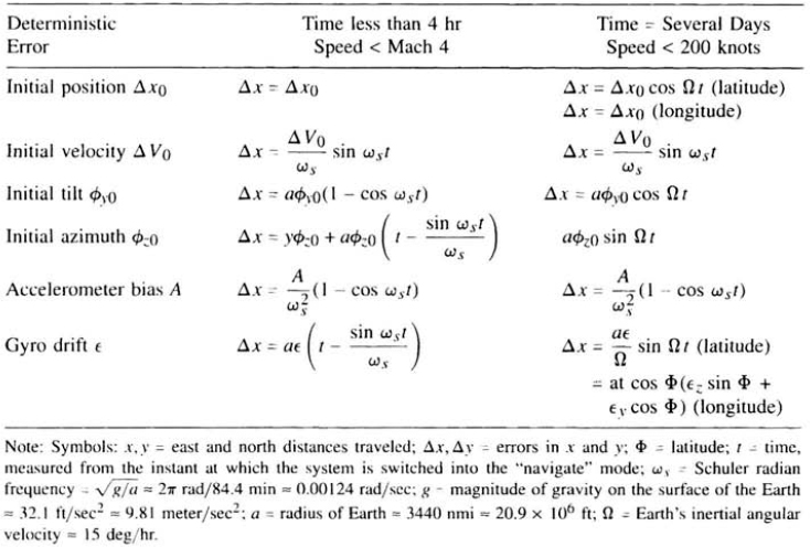
7.6.4 Total System Error

Section 2.8 discusses the definition of mean and circular-error-probability (CEP) horizontal errors, and their measurement from flight-test data. References [15, 17] discuss the errors present in strapdown systems in the late 1980s and early 1990s, including test results over a large number of flights. Strapdown RLG-based inertial navigators conforming to the military specification of Ref. [62] demonstrated a CEP better than 0.3 nmi/hr accuracy during 4097 flight tests performed by the Springfield, IL, Air National Guard during 1991 and 1992. These systems have also demonstrated an MTBF approaching 4000 hours in military environments [15].

7.7 ALIGNMENT

An inertial system solves the five simultaneous second-order differential equations for the attitude and horizontal position of its platform. Hence, ten initial conditions are required in order to initialize the computer, as discussed below:

1. Two initial position coordinates. When aligning an inertial system in a stationary vehicle on the ground, the initial conditions are obtained from a survey of the launch site. Airborne position fixes can be obtained by visual or radar checkpoints or by the use of radio-navigation aids.
2. Two initial velocity coordinates. When aligning on a stationary vehicle, the initial velocity relative to the Earth is nominally zero. When aligning on a moving aircraft, velocity is measured with a Doppler radar (Chapter 10), a succession of radio-aid fixes (Chapter 4) or a GPS velocity measurement (Chapter 5). When aligning on an aircraft carrier, a ship's inertial navigation system is usually the reference and a lever-arm correction must be made for the aircraft's position on the deck.
3. Three platform orientation coordinates. Terrestrial inertial navigation systems are initialized by leveling (two coordinates) and azimuth aligning (one coordinate) to a convenient reference. Leveling is accomplished by rotating the inertial platform (analytic or mechanical) until the average acceleration along each of the two horizontal platform axes read zero, at which time the navigation frame is deemed level. In a mechanical platform, this corresponds to a null output of the two horizontal accelerometers. In a strapdown system, none of the accelerometer outputs are necessarily nulled. Rather, their outputs, resolved onto the horizontal axes of the analytic platform, are driven to zero. Azimuth alignment is accomplished by any of several procedures discussed below.
4. Three orientation rates. These initial conditions are implicitly determined by the values of the gyro drifts at the instant of switching from the “align” mode to the “navigate” mode. These rates are not always measurable during alignment and can cause navigation errors.

The presence of initial-condition errors causes position errors, which propagate according to Table 7.2. To achieve 1 nmi/hr navigation accuracy, initial errors should be limited to 5 arcmin in azimuth, 10 arcsec in tilt, and 1 knot in velocity.

Several methods of alignment are used for aircraft:

1. Leveling and gyrocompassing using gyros and accelerometers. This procedure is analyzed in Sections 7.7.2 and 7.7.3. It can be performed on a stationary or moving vehicle, except near the Earth's poles.
2. Transfer alignment, relative to a master platform. A secondary inertial navigation system may be aligned to a master unit (e.g., an aircraft unit to a shipboard unit or a low grade unit to a higher accuracy system). The transfer alignment can be accomplished via acceleration/ velocity matching and/or via attitude matching, Section 7.7.4. Large lateral accelerations, such as exist on the deck of an aircraft carrier, are usually needed to increase the signal-to-noise ratio during acceleration or velocity matching.
3. Memory alignment, in which the attitude angles recorded during a previous alignment are stored. This procedure saves time, because it can be done in seconds, but it is limited by the angular repeatability of the aircraft landing gear and inertial-system shock-mounts. The aircraft must not be moved between the time of precise alignment and the time of memory alignment. This method is not suitable for use on ships or in flight.
4. Runway alignment when the aircraft taxis on a runway or taxiway of known heading prior to takeoff. Alignment procedures can take advantage of turns and stops to estimate errors. Stops at different headings provide opportunities for refining the platform heading estimates and fine-tuning the gyro-bias estimates.
5. Optical alignment. An inertial system can be aligned relative to an external optical line of sight within a few seconds of arc. It is impractical, however, on ships and aircraft because of the necessity for optical access and the inconvenience of establishing theodolite sites. Optical alignment of terrestrial aircraft guidance systems is sometimes used in conjunction with platforms that have star-trackers mounted on the stable element. Navigation systems for space applications often make use of optical alignment.
6. Portable platform alignment for rapid alignment. This procedure was developed in the 1960s. It used a portable platform that was aligned in a ready-room and carried aboard the aircraft at flight time. Portable platforms are rarely if ever implemented because they must be precisely installed in an accessible location and because they accumulate drift while being carried to the aircraft.

Fast warm-up is an important military requirement for interceptors, strategic bombers, and carrier-based aircraft. In older gimballed systems, warm-up time was limited by the interval taken by the inertial instruments to reach thermal equilibrium, typically 30 minutes. The warm-up rate could not be too high because of the detrimental temperature gradients induced by rapid application of heat. Use of the system before it had warmed up resulted in large navigation errors. In some systems, heaters were placed on the instruments in order to achieve rapid thermal stabilization. Those systems were capable of full performance within a few minutes. In the early 1980s, the shift to strapdown systems based on optical gyroscopes, and high-speed microprocessors eliminated the need for thermal stabilization. Since optical gyros exhibit much lower thermal sensitivity than their mechanical counterparts, it is possible to model errors such as bias, scale factor, and misalignments using polynomial functions of temperature in a flight computer. Typically, second-through fourth-order functions are implemented to model instrument errors during warm-up.

Strapdown accelerometers are also designed with low thermal sensitivity and repeatability that permit thermal modeling. A factory calibration procedure (Section 7.4.1) derives the temperature coefficients that are loaded into a nonvolatile memory. Sensors measure temperatures at key locations within the instruments. During system operation, the calibration coefficients are applied to polynomials of temperature, Equation 7.47. Thermal compensation in 1996 permitted better than 1 nmi/hr performance with extremely rapid reaction (four minutes). Only the most accurate systems included heaters for thermal stabilization.

7.7.1 Leveling

The purpose of leveling is to orient the platform (analytic or mechanical) with respect to gravity.

Coarse Leveling

Gimballed Platform In leveling a gimballed platform, the gimbal servos rotate the stable element in order to null the outputs of the horizontal accelerometers. To reduce alignment time, the gimbals are first slewed to null the pickoffs (e.g., synchros) or the accelerometers. This “coarse leveling” can be performed at slew rates of several hundred degrees per second, limited only by the construction of the mechanical gyros. Synchro nulling is used when the attitude of the platform within the vehicle at rest is nominally level. The accuracy of the coarse-leveling process is limited by (1) errors in mounting the platform to the vehicle, (2) shock-mount angular deflection and nonreturnability, (3) synchro errors, and (4) rocking of the aircraft on its landing gear and tires, induced by wind gusts or by personnel climbing on the aircraft.

Analytical Platform In a strapdown system, the orientation of the accelerometers is determined by the attitude of the vehicle and cannot be adjusted. Instead, leveling consists of rotating the transformation quaternion or direction cosine matrix that relates the instrument axes to the locally level navigation axes. Leveling is accomplished by adjusting the analytic platform in such a way that the accelerometer outputs transformed to horizontal platform axes are nulled. Estimates of the vehicle's pitch θ and roll ϕ are made using the accelerometer outputs (body frame readouts):

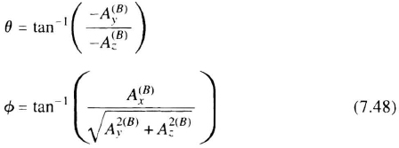
where x is forward, y is transverse (positive out the right wing), and z is down. Based on the pitch and roll so-derived, the system's body-to-navigation coordinate transformation (quaternion or direction cosine matrix) is initialized. The process of coarse-leveling a strapdown system requires only a few seconds, the time it takes to obtain a good measure of acceleration. The accuracy of coarse leveling is limited by accelerometer errors and noise as well as by motion of the vehicle.

Fine Leveling In a gimballed system, the outputs of the accelerometers generate gyro torque commands. The gyros, in turn, drive the gimbal servos until two accelerometers are level and, on a stationary vehicle, measure no average acceleration. The maximum precession rate of the gyro torquers limits the alignment speed.

In a strapdown system, the accelerometer outputs are transformed through the attitude matrix to form the analogue of gimbal-mounted accelerometer outputs. The computed horizontal accelerations are used to “torque” the analytic platform (i.e., rotate the platform axes by recomputing the attitude quaternion or direction cosine matrix) to maintain zero level-axis accelerations.

Figure 7.26 shows one axis of a fine leveling loop for a stationary vehicle. Tilt errors cause computed velocity to build up. Reducing tilt (via gyro torquing in a gimballed system or via quaternion torquing in a strapdown system) rotates the platform axes into alignment with the navigation axes. The addition of feedback to the velocity integrator provides the damping that forces the oscillations to decay.

The choice of gains K₁ and K₂ represents a tradeoff between rapidity of leveling and noise immunity. A Kalman mechanization computes time-varying optimal gains based on the system noise and error model. Nonetheless, fixed precomputed gains usually yield acceptable leveling performance without a Kalman filter. Leveling on a stationary vehicle takes approximately 30 to 60 seconds. Vehicle motion lengthens the required leveling time. Leveling-loop errors result from level-axis accelerometer or gyro errors, or from other horizontal disturbances. During ground alignment, rocking of the aircraft on its landing gear may be induced by wind gusts, machinery, and personnel boarding the aircraft.

Figure 7.26 Second-order fine leveling loop.

The response of the second-order leveling loop shown in Figure 7.26 is given by

where

δϕ	is the tilt error
ϕ0	is the initial tilt
A	is an uncompensated accelerometer bias
Vo	is the initial velocity error
ε	is an uncompensated gyro bias error
s	is the Laplace transform operator

7.7.2 Gyrocompass Alignment

In addition to orienting the platform (mechanical or analytic) with respect to gravity, it is also necessary to initialize its orientation relative to north. Azimuth alignment consists of either rotating the platform around the vertical to a desired direction (e.g., true north or a great-circle flight track) or to determine the orientation relative to the desired direction. The latter is applicable to wander azimuth systems in which the initial wander angle α₀ is calculated during alignment. Gyrocompass alignment usually consists of the following steps:

1. Coarse leveling
2. Fine leveling
3. Gyrocompassing during which fine leveling continues

In strapdown systems, steps 2 and 3 are executed simultaneously, using a Kalman filter to provide the proper weighting. Gyrocompass times are typically 3 to 8 minutes for stationary alignment of military vehicles (some of which have quick-alignment requirements), 1 to 2 minutes for in-flight alignment with high-quality velocity references, and 10 minutes for stationary alignment on commercial airliners.

Gyrocompass alignment on a stationary vehicle is based on the fact that if a platform is to remain level with respect to a rotating Earth, then it must rotate at Earth rate. For a level platform at latitude Φ and azimuth α, the steady-state platform level rates are (see Figure 7.21a)

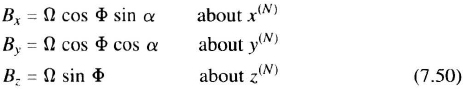
A stationary gyrocompass loop can be mechanized as an extension of the leveling loops as shown in Figure 7.27. Tilt rate states B_x and B_y estimate the platform rates necessary to maintain a level platform while B_z maintains azimuth. Azimuth α can be computed from

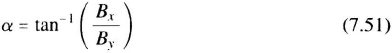
If latitude is known, then an estimate of the north gyro bias error may also be obtained:

Computed gyro bias error in the north direction is often resolved into instrument axes and applied as compensation (known as mini-bias) upon entering the navigation mode. In a single-position gyrocompass alignment, gyro bias error in the east direction cannot be distinguished from azimuth bias. Any uncompensated component of gyro bias in the east axis will result in a heading error.

An alternative mechanization may be used for gyrocompassing in which the platform is rotated so as to null α (i.e., to make B_x = 0). This can be accomplished via a mechanical rotation in a gimballed platform or by quaternion rotation in a strapdown system. It cannot be done accurately above about 70-deg. latitude.

The choice of fixed gains in the gyrocompass filter depends on the noise characteristics of the instruments and on the operating environment. Reference [23] presents a detailed discussion of conventional gyrocompass loops and their response characteristics. Since the 1970s, systems have employed variable-gain Kalman filters for the fine leveling and alignment process. Kalman filters can be mechanized to align at zero velocity (on stationary vehicles) or can be mechanized to accept external velocity or position fixes. A simple zero-velocity ground-align filter implements the model shown in Figure 7.27 but includes noise sources to calculate the optimum gains. Initial level errors and accelerometer noise limit the first stages of alignment (i.e., the first 30 seconds). The tilt gains peak in the first few seconds, then die out as the system levels. In the steady state, heading estimation is limited by the gyro noise. The tilt-rate gains start out low then grow within the first minute. Heading is captured during this time. The tilt rate gains then tail off slowly to allow fine tuning of the tilt rate estimates (and hence heading). A system with a gyro white noise of (typical of a navigation grade optical gyroscope) and gyro-bias accuracy of better than 0.01 deg/hr can gyrocompass to a heading accuracy of better than 1 mrad in less than 8 minutes at low and mid-latitudes.

The state equations for the diagram in Figure 7.27 are given by

This matrix equation is used in the Kalman filter equations [14] (see Chapter 3), along with estimates of the initial state uncertainties and noise terms. Noise sources that must be considered include velocity noise (due to aircraft motion and accelerometer quantization) which drives the position states, accelerometer white noise and gyro quantization which drive the velocity states, and level-axis gyro white noise which drives the tilt states.

In summary, a typical alignment consists of leveling (sometimes broken down into coarse and fine leveling), and gyrocompassing. In the alignment process, the gravity vector and the Earth-rate vector serve to define the coordinate reference frame. Modern strapdown navigators of the 1-nmi/hr variety align in 3 to 10 minutes on a stationary vehicle while achieving level accuracies of approximately 5 arcsec and heading accuracies of 1 mrad at mid-latitudes. Heading accuracy degrades in the polar regions due to the weak north component of Earth rate.

Chapter 3 describes multisensor navigation systems that mix inertial measurements with GPS or Doppler radars. These systems level and gyrocompass the platform coordinates continuously. In the event of loss of power or equipment failure, the multisensor system raises its gains for several minutes to realign, after which navigation proceeds with optimal gains. In-flight align times are typically on the order of one to two minutes but depend on the maneuvers executed and on the quality of the reference sensor.

7.7.3 Transfer Alignment

Some vehicles contain a high-quality inertial navigation system and one or more lower-cost units, for example, mounted on weapons that are to be released inflight. Transfer alignment is the process of matching the slave platforms to the master, using natural or deliberately-induced maneuvers of the vehicle. Transfer alignment consists of simultaneous leveling and gyrocompassing. Accuracy is limited by the flexural vibration of the vehicle, which causes the outputs of the master and secondary accelerometers to differ slightly even when the two platforms are aligned. Since the slave platforms are not co-located with the master, a lever-arm correction is necessary to compensate for the differences in velocity at the master and slave.

Figure 7.27 Two-axis, fourth-order gyrocompass loops.

The lever-arm velocity can be obtained by differentiating the lever-arm distance in navigation coordinates:

where

R(B)	is the lever-arm vector in body coordinates
R(N)	is the lever-arm vector in navigation coordinates
	is the transformation matrix between body and navigation coordinates

The term represents bending or flexing of the airframe. Difficulties in estimating usually preclude its inclusion in the lever-arm compensation. It represents an error in the transfer alignment.

In strapdown systems where the body-to-navigation direction-cosine matrix is updated rapidly (e.g., 200 times per second), an alternative form of compensation is preferred:

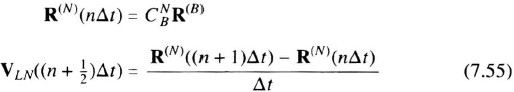
where V_LN is the lever-arm velocity in navigation coordinates. This mechanization avoids potentially noisy measurements of angular rate. Lever-arm acceleration may also be calculated by differencing V_LN.

where A_LN is the lever-arm acceleration in navigation coordinates. This computation avoids the use of an angular acceleration measurement. The lever-arm correction is particularly important when aligning on an aircraft carrier where an aircraft INS is being aligned to the ship's inertial navigation system. The limitations of the lever-arm compensation include the lever-arm flexure as well as uncertainties in the distances involved.

7.7.4 Attitude and Heading Reference Systems (AHRS)

Some inertial systems are configured only to provide attitude. Such systems use lower accuracy gyroscopes. Inertial navigation systems may also revert to AHRS operation in case a fault is detected in the system or degraded navigation performance becomes apparent. In AHRS mode, it is assumed that horizontal accelerations are transient conditions (Chapter 9). The system is maintained in a “loose” leveling mode using gyros to track rapid attitude changes. In the steady state, the accelerometers maintain the platform level. A magnetic compass or other heading reference maintains long-term azimuth (Chapter 9). A second-order AHRS leveling loop is mechanized in the same manner as the fine-leveling loop discussed in Section 7.7.1, illustrated in Figure 7.26, and discussed in Section 9.3. Time constants on the order of 30 seconds are used, and cutouts are usually implemented to open the leveling loops when large accelerations or angular rates are detected. Reference [30] discusses an AHRS implementation and reference [53] discusses a low-cost GPS/inertial system designed to provide attitude.

7.8 FUNDAMENTAL LIMITS

The accuracy of inertial systems cannot be improved indefinitely, even with the best instruments. Reference [26] shows that the most severe limit on position measurement is the uncertainty in the Earth's gravity field in the region of operation, since accelerometers cannot distinguish between kinetic acceleration and gravity. Angular errors in the measurement of inertial space are primarily limited by the precession of the equinoxes and the migration of the Earth's pole. These errors are 5 × 10⁻⁵ deg/hr, equivalent to 100 ft position error [26].

Measurements of azimuth and tilt of the vehicle are typically limited by the angular returnability of the shock-mounts, the installation accuracy, and the flexure of the vehicle. These errors typically range from 1 minute of arc to 0.5 deg.

7.9 FUTURE TRENDS

Trends in inertial instruments are discussed in Section 7.3.5. Several trends are emerging for inertia! navigation systems:

1. Miniaturization of strapdown systems. Technological advances permit smaller gyros (e.g., fiber optic) to be used. Advances in computer and electronics packaging permit the miniaturization of system electronics, resulting in lower volume and power consumption.
2. Integrated systems, which include inertial sensors and GPS receivers, provide high-bandwidth, low-noise navigation and attitude data with longterm accuracy ensured by GPS [54].
   • Low-cost civil navigators (using 2-10 nmi/hr inertial sensors) will rely heavily on GPS, fiber-optic gyros, and micromachined accelerometers. They will be used in many military vehicles as well.
   • High-performance military navigators with precise inertial instruments will be used in hostile conditions where reliable GPS signals may not be available.
   • Inertial systems are being incorporated into landing aids (see Chapter 13).
3. Multi-function inertial systems. In addition to providing data for inertial navigation, the sensors are capable of supplying high-quality information for flight control, weapon delivery, and compensation of synthetic aperture radar. Excellent angle resolution is also possible for pointing and tracking applications. Rigid mounting of the angular sensors is required.
4. Throwaway inertial systems with GPS aiding will be used for a wide variety of applications including munitions and intelligent weapons. These low-cost systems will be based on fiber-optics and micro-machined sensors. Multi-axis gyro/accelerometer combinations employing silicon micro-machining may be acceptable.

When Com-Nav satellites, that supply intermittent radio fixes, supplant GPS, precise inertial navigation will be needed between fixes on commercial aircraft. These inertial navigators may take the form of micromachined panel-mounted instruments.

PROBLEMS

7.1. The following questions relate to accelerometers:

• (a) An accelerometer is mounted on the table of a centrifuge with its input axis horizontal and radially outward. What is its steady-state output in terms of the radial dimension and the angular velocity of the centrifuge about the vertical?

  Ans.: ω²R.

• (b) The input axis is rotated 45 deg downward so that it lies in the vertical plane containing the centrifuge axis. What is the steady-state output?

  .

• (c) The pendulosity of an accelerometer is mb = 10 g-cm, and the moment of inertia of the pendulum about its pivot axis is 20 g-cm². Calculate the stiffness of the restoring electronics that would give a deflection of 10 arcsec at 5 g. Calculate the undamped natural frequency.

  Ans.: 4.9 × 10³ dyne-cm/arcsec, 1.1 kHz.

7.2. The following questions relate to gyroscopes:

• (a) What is the scale factor of a square ring laser gyroscope operating at λ = 630 nm and with a pathlength of 30 cm in terms of seconds of arc per count (half-wavelength)?

  Ans.: 1.73 arcsec/count.

• (b) What path length is needed to obtain the same scale factor with an equilateral triangle RLG operating at the same wavelength?

  Ans.: 39.0 cm.

• (c) What is the maximum gyro random walk coefficient that will permit measurement of angular rate in a three-minute averaging period with a measurement standard deviation of less than 0.005 deg/hr?

  .

• (d) A mechanical gyroscope has H = 2 × 10⁶ g-cm². What residual torque is allowable to achieve a drift rate of 0.005 deg/hr?

  Ans.: 0.05 dyne-cm.

7.3. The following questions relate to analytic platforms:

• (a) Given the navigation coordinates shown in Figure 7.21 with α = 0, an aircraft is flying level in the north direction. What is the body-to-navigation quaternion (assume x-body is foward, y-body is out the right wing, and z-body is down)?

  Ans.:

  

• (b) What is the direction cosine matrix corresponding to the condition in (a)?

  Ans.:

  

• (c) Given a 50-Hz sinusoidal acceleration with amplitude a₀ = 2.5 g along the z-axis and a sinusoidal angular displacement in the same phase of amplitude θ₀ = 300 µrad about the y-axis, what is the sculling rectification of the x accelerometer?

  Ans.: 375 µg.

• (d) For the conditions in (c), calculate the net error resulting from a velocity transformation algorithm executing at 250 Hz. What is the error if the transformation executes at 100 Hz?

  Ans.: 24 µg, 136 µg.

• (e) An aircraft performing S-turn maneuvers generates a coning rate of 25,000 deg/hr about the wing axis. Assuming the maneuvers last 10 minutes, what tilt error is generated by a 5 µrad gyro nonorthogonality error? Assuming no other error sources, what is the position error exhibited at the end of the maneuver? What is the position error 42.2 minutes after the end of the maneuver?

  Ans.: 331 µrad, 0.11 nmi, 2.4 nmi.

7.4. The following questions relate to gyrocompass alignment:

• (a) At a latitude of 30 degrees, what is the approximate azimuth error resulting from a 0.01 deg/hr east gyro bias error in a stationary ground alignment?

  Ans.: 0.044 deg ≈ 2.6 arcmin ≈ 0.77 mrad.

• (b) What would the heading error be at 80 degrees latitude?

  Ans.: 0.22 deg ≈ 13 arcmin ≈ 3.8 mrad.

• (c) Given a gyro random walk coefficient of , what is the minimum alignment time required to attain an azimuth standard deviation of better than 0.7 mrad at 45° latitude?

  Ans.: 261 sec.

• (d) A strapdown system at 45-degrees latitude is aligned at a heading of 30 degrees. The x body-axis gyro has a bias error of 0.02 deg/hr. What is the resulting heading error during gyrocompass alignment? What bias corrections are computed for the gyros using mini-biasing?

  Ans.: –0.054 deg, x gyro 0.015 deg/hr, y gyro −0.0086 deg/hr.

• (e) A strapdown system at 34-degree latitude is aligned at a north heading. The x gyro has a bias error of 0.01 deg/hr and the y gyro has a bias error of 0.007 deg/hr. What is the heading error of the system? After alignment the system is switched to navigate mode with no minibiases used and immediately rotated 180 degrees in azimuth. What are the north and east position error growth rates neglecting Schuler oscillations? What are these rates if minibiases are used?

  Ans.: −0.032 deg, north 0.84 nmi/hr, east −0.6 nmi/hr; north 0.84 nmi/hr, east 0.00 nmi/hr.