8 Air-Data Systems

8.1 INTRODUCTION

An air-data system consists of aerodynamic and thermodynamic sensors and associated electronics. The sensors measure characteristics of the air surrounding the vehicle and convert this information into electrical signals (via transducers) that are subsequently processed to derive flight parameters. Typical flight parameters calculated by air vehicles include calibrated airspeed, true airspeed, Mach number, free-stream static pressure, pressure altitude, baro-corrected altitude, free-stream outside air temperature, air density, angle of attack, and angle of sideslip. This information is used for flight displays, for autopilots (flight-trajectory control and control-loop gain adjustment), for weapon-system fire-control computations, and for the control of cabin-air pressurization systems.

Air-data systems are an outgrowth of the airspeed indicator and altimeter used in early aviation. In those primitive, pneumatically driven instruments, the computation was performed by nonlinear spring mechanisms incorporated into specially designed bellows, which expanded or contracted in response to changes in sensed pressures, thereby moving the dials of the flight instruments. In the late 1950s, analog computers were interposed between the pressure sensors and flight instruments. The transducers and computation elements found in typical analog air-data computers of that era were documented in the first edition of this book [27]. In those designs, servo-driven cams or nonlinear potentiometers computed parameters such as altitude, airspeed, and Mach number. In the 1990s, all computation and data management are digital and based on microprocessor technology. Indeed, the miniaturization made possible by this technology is tending to obsolete the air-data computer as a separate entity. New avionics architectures are incorporating air-data functions into other subsystems such as inertial/GPS navigation units or are packaging the air-data transducers into the flight-control computers.

Regardless of how the air-data functions are packaged, they provide flight-critical information and therefore are implemented with appropriate redundancy and automated fault detection and isolation. Air-data systems can be found in every class of air vehicle, from combat fighters and helicopters to manned spacecraft such as Space Shuttle Orbiter. Their implementation in commercial jet transports uses ARINC standard specifications that are also used in business aviation. Each type of aircraft has unique challenges, primarily in regard to the accuracy of measuring the basic aerodynamic phenomena.

8.2 AIR-DATA MEASUREMENTS

8.2.1 Conventional “Intrusive” Probes

All of the air-data parameters that are relevant to flight performance are derived by sensing the pressures, temperatures, and flow direction surrounding the vehicle. Free-stream pressures and temperatures are required for the computation of static air temperature, altitude, airspeed, and Mach number. Because air is moving past the aircraft, the pressure at various places on the aircraft's skin may be slightly higher or lower than free stream. Figure 8.1 illustrates the probes typically deployed around the skin of an aircraft. They sample static pressure (via static ports), total pressure (via the pitot tube), total temperature (via the temperature probe), and local flow direction (via the angle-of-attack and sideslip vanes). All of these sensing elements, except for the flush-mounted static port, are intrusive because they disturb the local airflow. In flight testing of new aircraft, integrated air-data booms are often used to mount combinations of these probes forward of the flow which normally contacts the aircraft skin. Figure 8.2 illustrates such an instrumentation boom that would normally be located at the aircraft nose. The angle-of-attack and angle-of-sideslip vanes are self-aligning, measuring the direction of local flow. Total pressure must be measured at the front opening on the pitot tube which extends directly into the air flow, but at an angle with respect to the relative wind. That angle, defined by sideslip β and angle-of-attack α does not usually produce any significant inaccuracies as long as α and β are within ±10 degrees. In applications where α and β excursions are large, then special booms containing a gimbaled pitot tube can be used. Such tubes contain wind vanes or may be servo driven to align with the relative wind. Typical applications of self-aligning pitot tubes are in developmental testing for experimental aircraft, or for high-angle-of-attack fighter aircraft. Non-intrusive probes are discussed in Sections 8.5.2 and 8.5.3.

8.2.2 Static Pressure

Static pressure is the absolute pressure of the still air surrounding the aircraft. To obtain a sample of static air in a moving aircraft, a hole (static port) or series of holes are drilled in a plate on the side of the fuselage or on the side of the pitot tube probe which extends into the free airstream. These sensed static pressures will differ from the free-stream values for reasons noted above. That difference is referred to as the static defect. The location of static ports is selected by wind-tunnel tests and by tests at numerous locations on actual aircraft. The location of a static port on helicopters or on fixed-wing aircraft that operate at very high angles of attack is especially difficult because of unusual local flow phenomena. Even with an optimum static source location, a large static defect usually remains, which is a function of Mach number, angle of attack, and aircraft configuration (flap deployment, wing stores, etc.). Because static defect is predictable, it can be corrected in the air-data computations. Techniques for correcting such errors are covered in Sections 8.3 and 8.4.

Figure 8.1 Air-data system, input probes and vanes (probes courtesy, Rosemount, Inc.).

Figure 8.2 Typical nose-mounted air-data boom with pressure probes and flow-direction vanes.

8.2.3 Total Pressure

The terms total pressure, stagnation pressure, or pitot pressure refer to the pressure sensed in a tube that is open at the front and closed at the rear. The pitot tube is illustrated in Figures 8.1 and 8.2. When the static pressure ports and the pitot tube are combined into a single probe, the instrument is called a pilotstatic tube. Such tubes are electrically heated to prevent ice formation. Pipes in the aircraft, referred to as the pneumatic plumbing, carry the sensed pressure to transducers associated with the air-data computations and also to direct-reading airspeed indicators. Since the 1970s, large aircraft carry direct-reading, pneumatic instruments at the crew stations to backup the computer-driven instruments. In subsonic flight, a pitot tube's recovery of total pressure is reasonably accurate for typical variations in angle of attack and Mach number; hence, compensations to correct static defect are generally not required. At supersonic speeds, the pressure sensed within the tube is ideally the pressure that develops behind a normal shock wave. Design and calibration of the pitot tube orifice to achieve the desired shock wave is difficult, so measurement errors in total pressure are higher at supersonic speeds and must be compensated.

Total pressure is used to compute calibrated airspeed V_c and Mach number M. Impact pressure q_c is measured with a differential pressure transducer:

where p_t is the total pressure and p is the static pressure. Impact pressure differs from dynamic pressure q by compressibility factors. Dynamic pressure is often used in aerodynamic calculations because of its simplicity:

where ρ is the air density and V is the true airspeed, often referred to as V_t. There are many forms for the analytical representation of q_c. It is usually shown [4, 24, 30] for subsonic flight as Equation 8.3

and for supersonic flight as Equation 8.4:

TABLE 8.1 Standard atmosphere properties

where γ is the ratio of specific heat of air at constant pressure to specific heat at constant volume; for air, γ = 1.4.

From Equations 8.2 through 8.4, we can obtain the definitions of the various types of airspeed encountered in aviation practice and theory: Calibrated airspeed V_c is defined from Equations 8.3 and 8.4 as the airspeed V that would result from the measured value of q_c if the aircraft were at standard sea level conditions (see Table 8.1). Indicated airspeed V_i is identical to V_c, except that it represents the readings of an instrument that has not been correct for pitot-static and other errors. Another term often used by aerodynamicists is equivalent airspeed V_e. This is a theoretical parameter that can be computed if desired:

Equivalent airspeed approaches calibrated airspeed at low Mach numbers. With some algebraic manipulation, the parts of Equations 8.3 and 8.4 that multiply ρV²/2 can be shown to be functions of Mach number M [2, 30]. The departure of q_c from q can be observed from Figure 8.3, which plots the ratio q_c/q versus Mach number. There are many ways to manipulate the variables in the above equations to derive airspeeds but a set of standard equations is usually used (Section 8.3).

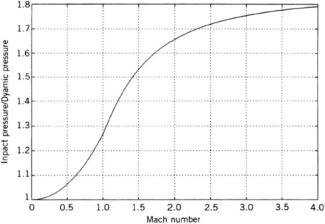
Figure 8.3 Ratio of impact pressure to dynamic pressure versus Mach free stream.

8.2.4 Air Temperature

Outside air temperature, referred to as static air temperature T_s and sometimes as OAT, is required for the computation of true airspeed. It is also used in the computation of air density, which is required for some types of fire-control aiming solutions. The temperature measured by a thermometer on the exterior of a moving aircraft is higher than the free-stream air temperature because of frictional heating and compression of the air impinging on the thermometer (altered by radiation from the thermometer to the sky and airframe). A typical temperature probe, illustrated in Figure 8.1, is installed to point along the local streamline and compresses the impacting air to zero speed, thus causing a “total,” or “stagnation,” temperature to exist at the thermometer. To avoid time lags in the temperature measurement, a leakage hole at the rear of the probe allows for a rapid air change. Probes may be mounted on the wing tips, vertical tail, forward fuselage, or other locations where the local Mach number is the same as the free-stream Mach for all expected flight attitudes and speeds. The temperature actually measured by the thermometer is T_m [2, 30].

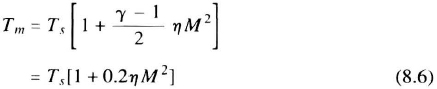
where absolute temperature is in Kelvins or Rankines, M is the local Mach number, and η is the recovery factor of the probe. The recovery factor accounts for frictional heating, re-radiation, and nonisentropic compression of the air. η is measured empirically, and when independent of Mach number and angle of attack, it does not contribute to any errors in the computation of static air temperature. Temperature probes are available with η values ranging from about 0.7 to greater than 0.99. For high values of η, special shields reduce radiation heat exchanges. Electrical heaters used for deicing must be isolated from the thermometer element. The thermometer is usually a small coil of wire whose resistance varies with temperature. The resistance variation is detected in a bridge circuit, whose excitations and signal processing are located in a signal-conditioning box or the computer. Moisture, water ingestion, and icing are significant error sources that are reduced by a variety of design techniques, including heaters. Substituting numbers into Equation 8.6 shows that the 0.2 M² term accounts for 12.8% of measured temperature at M = 0.8. A 1.0°C error in temperature will result in a true airspeed error greater than 1.0 knot at typical transport–aircraft flight conditions.

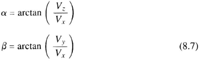
8.2.5 Angle of Attack and Angle of Sideslip

Angle of attack is the angle, in the normally vertical plane of symmetry of the aircraft, at which the relative wind meets an arbitrary longitudinal datum line on the fuselage. Usually that datum line is the aircraft's X-axis, the orthogonal line out the right wing from the center of gravity is the Y-axis, and the Z-axis is downward to complete a right-hand coordinate frame. The angles of attack α and sideslip β can be defined in terms of air velocity components along these axes, V_x, V_y, and V_z.

The pivoted vane, illustrated in Figure 8.1, measures local flow angle and is the most commonly used method of measuring α or β. Maximum angle-of-attack boundaries define the aircraft's low-speed flight envelope. When α sensors are installed on aircraft, they are usually part of an independent stall warning or stall control system. Since such systems are flight critical (also called safety critical), redundant sensors are usually installed. Other methods of measuring α and β are discussed in Section 8.5. Engine inlet controls also use α measurements that tend to be safety-critical in supersonic flight.

Sideslip sensors are usually used only in developmental flight test instrumentation. In normal operation, sideslip is approximated by a body-mounted lateral accelerometer (y-axis) and displayed on the pilot's ball bank indicator. Automatic flight control systems compute sideslip from inertial measurements and include sideslip control as part of their lateral-directional control loops. Many yaw dampers use mechanizations based upon the estimated rate of change of β from measurements of lateral acceleration, bank angle, and inertial yaw rate rather than obtaining the desired information from a sideslip sensor. With fast computers, α and β can be estimated from the aircraft force and moment equations and the more commonly available inertial and airspeed measurements. Analytically derived α may supplement a vane sensor for redundancy.

8.2.6 Air-Data Transducers

Measurements of pressures and temperature must be accomplished by transducers that convert the sensed parameters into mechanical motions or electrical signals that are compatible with the various user subsystems. Figure 8.4 summarizes the evolution of transducers, starting with the early pneumatic indicators of altitude and airspeed. In these early instruments, the sensor mechanism and the computation function were combined. The dial whose displacement was proportional to altitude or airspeed (Figure 8.4a) included the computation of altitude or airspeed from the sensing of static pressure and impact pressure. That computation was accomplished by the use of nonlinear springs inherent in the pressure capsules or bellows and associated linkage mechanisms. By the 1950s, avionic systems began to require electrical signals proportional to altitude, airspeed and other air-data parameters. At first, attempts were made to attach electrical transducers such as synchros and potentiometers to these pneumatic instruments but technical problems associated with achieving required sensitivities soon led to servo-driven shafts whose rotation was proportional to the desired air-data parameters. These shaft-driven devices, illustrated by an altitude computing instrument in Figure 8.4b and a Mach computing instrument in Figure 8.4c, combined the sensing and the computation. These illustrations represent the force-balance sensors which dominated central air-data computers in the 1960s and early 1970s. More details of the physical mechanization of such sensors are given in the first edition of this book [27].

Figure 8.4d shows a typical digital computation of altitude using a class of pressure sensor that is usually referred to as a digital sensor. In reality, it is an analog sensor whose analog of pressure is frequency rather than displacement or voltage. Frequency can be encoded into a numerical value with greater precision than voltage. The introduction of digital air-data computers in the early 1970s produced a major improvement in accuracy, reliability, size, and weight. Accuracy improved because sensors could store precise calibration data, which remained with the sensing element in the form of a read-only memory (ROM) chip. Digital computation of the required functions is considerably more accurate and repeatable than electromechanical analog computation. Reliability increased because of the elimination of the motor-driven parts and their difficult test and calibration procedures. Size/weight advantages were a natural consequence of the elimination of electromechanical hardware, while improvement continues to be realized as computing and input-output chips become more powerful.

Figure 8.4 Evolution of air-data instrumentation: (a) Pneumatic instruments; (b) force-balance electromechanical altitude computation; (c) electromechanical Mach computation; (d) digital computation of altitude.

Figure 8.4d is a conceptual view of a vibrating-diaphragm sensor produced by Sperry Corp. (now Honeywell) for such aircraft as the Boeing 757, 767, 737-300/400, the F-15 and F-16 fighters, and other military, commercial, and general aviation aircraft. Another class of pressure sensor used in digital air-data computers is based on silicon piezo-resistive technology. One of the more difficult problems associated with achieving accuracy has been the temperature sensitivity of silicon. Designs that will work over very wide temperature ranges require balancing techniques in the bridge circuitry that detects the voltage unbalance generated by the silicon transducer. Some solutions use two bridges, one to measure the output of the pressure sensor plus its temperature drift, and a second bridge that does not receive a pressure input but only responds to the temperature changes. Another approach uses the piezo-resistive element as one arm of the bridge circuit and a second silicon element with “identical” temperature drift characteristics in the balance arm of that bridge. Accuracy of any precision pressure sensor is determined largely by the quality of the temperature compensation. Most silicon sensors produce electrical outputs that must be passed through analog-to-digital (A/D) converters. The conversion must be accurate to at least 16 bits (1 part in 65536), which is beyond the capability of 1996 successive-approximation converters. Because high bandwidth is not a requirement for air-data parameters, the slower, more precise dual-slope A/D converters were used.

High performance of all types of sensors over a wide temperature range requires compensation. If the calibration data are stored, then the temperature behavior of the sensing device must be stable and repeatable. This ultimately becomes a materials technology issue. Beryllium-copper capsules, used in the vibrating diaphragm sensor illustrated in Figure 8.5a, must be heat treated and “aged” before their properties become sufficiently stable for use in a production sensor. Silicon fabrication processes are the key to meeting cost and performance goals. The trend for future applications seems to favor solid-state sensors because they lend themselves to automated fabrication processes. The size advantage of the solid-state/silicon sensor is illustrated in Figure 8.5b, which shows two sensors produced by the same manufacturer to the same accuracy specifications.

8.3 AIR DATA EQUATIONS

8.3.1 Altitude

To determine altitude from static pressure, international standards have been established [5, 11, 32, 47, 48]. The standard atmosphere model gives the relationship between a height Z and properties of the atmosphere as the solution to a differential equation relating the difference in pressure dp between two altitudes, Z and Z + dZ, to the weight of that column of air, where ρ is the local air density and g is the acceleration of gravity:

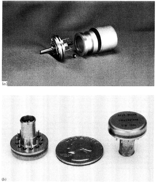
Figure 8.5 (a) Vibrating-diaphragm pressure sensor (courtesy, Honeywell, Inc.); (b) silicon piezo-resistive pressure sensor (courtesy, Honeywell, Inc.).

Solutions of this equation are given in [5, 11, 32]:

where the temperature T varies as a function of altitude, defined by the standard altitude model [5, 11, 30]. The standard atmospheric constants are given in Table 8.1, with pressures defined in terms of the height of a manometer column or in millibars (1.0 mbar = 0.1 kpascal = 0.0145 psi). Substituting the appropriate constants into equation 8.9, gives

for p in mm, Z in meters, and T in °C. The standard temperature gradient or lapse rate given in Table 8.1 defines a value of T for each altitude below 10,769 meters (35,332 ft), where the standard temperature becomes −55°C = 218 K = −67°F = 392.4 Rankines. Above this altitude, temperature remains constant until about 20 km and then begins to increase before decreasing again as the Earth's atmosphere effectively disappears. These higher-altitude temperature models play a role in hypersonic flight.

When standard temperatures are used for T, the value of Z for each p is called the pressure altitude. Air-data computers usually compute pressure altitude from look-up tables derived from Equation 8.9 with appropriate constants incorporated, including the standard function for T versus altitude, or pressure. A combination of the stored table of pressure and density for values of altitude spaced at 10- to 100-ft intervals will give more than adequate results by interpolation. Pressure altitude is the standard parameter used for vertical navigation in controlled airspace. However, density altitude is needed to assess an aircraft's performance margin. By reading or computing static air temperature and pressure, a corrected air density can be found:

The altitude corresponding to that density can be extracted from the look-up table; it is density altitude. An alternative way of computing density altitude is to enter the actual value of static air temperature for T in Equation 8.9 and compute Z using the existing value of static pressure p.

Another type of altitude produced by an air-data system is baro-corrected altitude, computed from pressure altitude by adding an offset. The offset is the deviation from standard sea-level pressure as computed from the difference between the barometric reading at a ground station and the standard barometer at that altitude. Baro correction is entered either in millibars or inches of mercury. Throughout the world, aircraft flying below 18,000 ft use a local barometric correction, while those flying above 18,000 ft set their altimeters to 29.92 in. of mercury.

8.3.2 Mach Number

The Mach number M is computed from the corrected pitot and static pressure measurements, P_t and P_s, respectively, where P_s ≡ p and p_t = p_s+q_c. The equations that define M can be derived from Equations 8.3 and 8.4 by recognizing that

where C_s is the speed of sound [2, 30]:

Substituting for V_t into Equations (8.3) and (8.4); with γ = 1.4, gives the expressions for subsonic and supersonic M that are computed by air-data systems. The subsonic Mach equation is

which can be rearranged to solve for M explicitly:

The supersonic Mach equation is

This expression cannot easily be solved explicitly for M, although it can be solved as a polynomial expansion of q_c/P_s. Many air-data computers store tables of q_c/P_s versus Mach obtained from Equations 8.13 and 8.15, using interpolation routines to extract M from the ratio of corrected pitot and static measurements. Figure 8.6 illustrates the Mach versus pressure-ratio relationships for both the subsonic and supersonic regimes, noting that at M = 1.0, both equations give the same result.

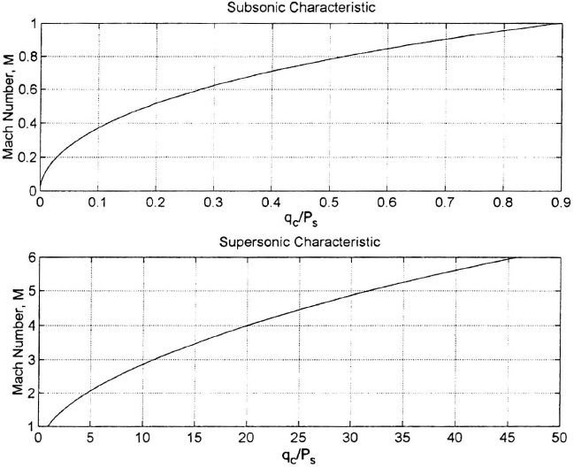
Figure 8.6 q_c/P_s versus Mach number.

8.3.3 Calibrated Airspeed

Calibrated airspeed V_c is defined from Equations 8.3 and 8.4 by letting V = V_c, p = p₀, and ρ = ρ₀. This will allow an explicit solution for V_c. Thus, for the subsonic case,

where C_s0 is the standard day, sea-level speed of sound (Table 8.1).

8.3.4 True Airspeed

True airspeed is usually computed from the relationship M = V/C_s. The value of M is computed from Equations 8.13, 8.14, and 8.15. The value of C_s from the computation of static air temperature was given as Equation 8.12, and T_s is

If T is in Kelvin, then knots.

In low-speed flight of aircraft and helicopters, the Mach number is not an appropriate flight parameter; hence alternative methods of computing true airspeed V_t are needed. The usual method is

where f and f₀ are compressibility factors containing the same parameters as in Equation 8.3 [2]. The ratio f/f₀ will approximate 1.0 at low speeds. Tables of ρ versus altitude are stored in the air-data computer.

8.3.5 Altitude Rate

Air-data computers usually provide an output identified as altitude rate. It is an outgrowth of early pneumatic rate-of-climb indicators, which differentiated a pressure by feeding it to a constriction in the tubing with an air chamber. This analog differentiation suffered from undesirable lags, so these instruments were replaced with “instantaneous vertical speed indicators” that mixed a signal derived from a Z-axis accelerometer with the constricted pneumatic measurement. With the advent of central air-data computers, altitude-rate signals were computed from altitude. Since the 1980s, altitude rate has been computed digitally from vertical acceleration and rate of change of pressure altitude (see Section 7.5.3).

8.4 AIR-DATA SYSTEMS

8.4.1 Accuracy Requirements

The most stringent demands on the accuracy of civil air-data systems come from the need to estimate pressure altitude with sufficient precision to support vertical separation in crowded airspace (Table 8.2). The key to accurate pressure altitude is the calibration of static defect errors. By contrast, calibrated airspeed, true airspeed, and Mach number are not used for navigation. Their accuracy is driven by flight performance/stall envelopes in takeoff and landing conditions. The components of true airspeed are often subtracted from those of inertially measured ground velocity to calculate instantaneous wind velocity in cruise conditions, which is useful for the on-board computation of fuel-optimal trajectories in flight-management computers. Mach number is used for programming of stabilizer position for speed stability, defining high-speed performance boundaries such as flutter onset, and for defining optimal cruise paths. Many commercial air-data specifications require outputs for maximum operational velocity (VMO) and maximum operational Mach (MMO) [3]. Table 8.2 summarizes typical accuracy requirements imposed on civil air-data computers since the mid-1970s that were unchanged into the 1990s. Accuracies specified for military air-data systems have, in general, followed the civil specifications, except for supersonic Mach number and airspeed. Those specifications are tailored to the aircraft mission and to probe calibration technologies. Mach number accuracy drops off at very high altitudes. In the supersonic flight regimes of fighters, Mach number accuracies of about 1.0% are typical. The level of performance in Table 8.2 implies calibration of the pitot and static sources. For civil transports, such calibration data are usually available. For military supersonic aircraft, complete probe calibration data are often lacking, especially for high acceleration maneuvers, and when aircraft stores (external pods, missiles and tanks) alter flow characteristics. Extensive flight testing is required to obtain this type of calibration data, and the high cost of such testing often compromises accuracy.

TABLE 8.2 Typical air-data computer accuracy requirements

8.4.2 Air-Data Computers

A typical central air-data computer (CADC) is a box containing: (1) the pressure transducers, associated excitation circuitry, and signal-conditioning circuitry, (2) the computer; and (3) the output drivers that are compatible with interfacing subsystems (Chapter 15). The box containing these elements includes fittings that allow the pitot and static pressure lines to connect to the computer's internal pressure transducers. Figure 8.7 illustrates a generic digital CADC. Its inputs are the pitot and static pressure tubes, a temperature probe signal (for the bridge circuit), a barometric setting (either from an analog baro-set potentiometer or from the aircraft's flight management system), and various aircraft configuration discretes. These discretes include flap deployment and external stores status for use in compensating raw pressure and vane readings. They also include “program pin” status, designated connector pins that allow a standard CADC to serve more than one aircraft type. Thus, pin i could recognize that the installation is in aircraft i, thereby activating its own pitot-static correction algorithm, or activating a unique signal interface. Input processing usually involves A/D conversion and packing of discrete signals into logic words, plus implementation of special serial data interfaces such as an RS 232 interface to an external software load and test environment. Input processing must also provide for the circuitry associated with the pressure transducers and vane signal conditioners. They include oscillators, clocks, counters, and precision excitation voltages, plus the interface to the internal computer bus that provides the pathway to the computer's memory. Output processing includes the port to the system data bus. In military applications, this has been a Mil-Std. 1553 bus, while commercial applications have used the ARINC 429 broadcast bus standard (although civil multiplex buses such as ARINC 629 have also appeared, Chapter 15). Special outputs such as synchro drivers for electromechanical instruments must also be accommodated by a CADC that is compatible with many aircraft types. One of these outputs, shown on Figure 8.7, is for the air-traffic-control transponder's Mode-C altitude-reply code. This format is needed by early vintage transponders, some of which remain in service despite the arrival of newer generation transponders that can receive the required altitude information over standard avionics busses. The CADC is also commonly used as the source of probe heater controls.

The air-data equations are solved in the processor subassembly, which contains the CPU, memory for the operational flight program (usually stored in electrically erasable programmable read-only memory, EEPROM), data storage memory (usually static random access memory, RAM), and nonvolatile RAM for storage of in-flight maintenance information. Since the computational elements of a CADC represent a small part of the hardware, new system architectures have eliminated the CADC as a separate subsystem (Section 8.4.3).

Figure 8.7 Functional block diagram of digital air-data computer.

The air-data software includes a considerable number of built-in test and monitoring algorithms for establishing the validity of all sensor inputs and processing. Other than this “overhead” software, typical computations performed by a generic CADC can be summarized with the following simplified sequence:

• Read probe data from transducers (P_t, P_s, α, β, T_t). Read internal transducer temperatures T_int and aircraft discretes D.
• Preprocess transducers (e.g., variable-frequency vibrating diaphragm)
  • Circuitry measures count N in time t
  • Frequency is N/t = F; F_p = P_s frequency, F_q = q_c frequency
  • P′_s is uncompensated static pressure, f₁(F_p, T_int, R), where R is the stored calibration curve for the specific transducer
  • P′_q is uncompensated impact pressure, f₂(F_q, T_int, R)
• Correct P′_s, q′_c, α₁ where α₁ = measured α
  • α = α₁ + Δα(α₁, D)
  • P_s = p = P′_s + f₃(α, M, D)
  • q_c = P′_q + f₄(α, M, D)
• Compute air-data parameters; initialize without Mach compensations, and allow solution to converge after 1 or 2 iterations. If the M compensations are large, and solution does not converge, compute a raw Mach solution from uncompensated p and q_c and use it in the pressure compensations.
  • M = f₅(q_c/p) from Equations 8.13–8.15
  • T_s = f₆(T_t, M) from Equation 8.17
  • C_s = f₇(T_s) from Equation 8.12
  • V_c = f₈(q_c) from Equations 8.3, 8.4, 8.16
  • V = f₉(C_s, M) from Equation 8.11
  • Pressure altitude Z = h = f₁₀(p) from Equation 8.9
  • Baro-corrected altitude is h_B = h + f₁₁ (baro correction)
  • Density is ρ = f₁₂(p, T_s) from Equation 8.10
  • Density altitude is f₁₃(ρ, h) from Equation 8.9

Computer throughput requirements vary with the choice of table look-up or polynomial equation solutions, iteration rate, and whether multi-rate computation executives are used. In the 1970s, a 100-KOPS, 16-bit microprocessor could perform the CADC functions using 10% to 50% of available time. In the 1990s, all CADC computations could execute in less than 1% of available time. The program and the aircraft-related compensation constants can be stored in less than 20,000 bytes of memory.

8.4.3 Architecture Trends

As microprocessors became smaller and cheaper, it became possible to package them with probes and transducers. The result is a distributed air-data system that replaces the CADC. A key feature is the packaging of signal-processing functions with or adjacent to the probes. Mechanization of such systems may be with “smart probes” whose integral electronics provide the probe and transducer calibrations, plus the digital interface. Figure 8.8 illustrates this concept with dual-redundant probes and vanes. Such an architecture provides corrected pressure, temperature, and angle-of-attack data to a flight control computer that computes altitude, Mach, calibrated, and true airspeed. It can also compute other standard air-data parameters and transmit them to flight management computers, mission computers, or other subsystems.

A major advantage of distributed architecture is the elimination of pneumatic plumbing to the CADC boxes. Reliability and maintenance problems, including water drains, are eliminated. Electrical wiring weighs less than tubing and the electrical transmission of pressure information eliminates lags associated with long lengths of tubing. These lags are negligible with minimum-volume pressure transducers. For example [39], a tube length of 12.70 meters, tube inner diameter of 9.5 mm, and a transducer volume of 100 cm³ (large for contemporary designs) will produce a lag time-constant of 0.008 sec at an altitude of 10,000 ft (3048 meters), and 0.187 sec at an altitude of 80,000 ft. (24384 meters). Even if the lag were significant, it could be corrected with blended inertial measurements.

The Boeing 777 has a partly distributed air-data architecture. Miniature air-data processing modules are located in the vicinity of the probe on the aircraft structure. The modules contain transducers and signal-processing circuitry. They compensate the transducers, control probe heaters, and interface with the aircraft's data bus. A module's output transmits to the aircraft's integrated inertial/air-data unit [36] via an ARINC 629 data bus (Chapter 15).

Figure 8.8 Smart-probe architecture for distributed air-data system.

8.5 SPECIALTY DESIGNS

8.5.1 Helicopter Air-Data Systems

Helicopter air-data systems differ from their fixed-wing counterparts primarily in the implementation of airspeed measurements at low speeds, including the inference of winds while the aircraft is hovering. Unlike fixed-wing aircraft, where a knowledge of airspeed is essential for safe flight, a helicopter's airspeed is not an essential pilotage quantity, except for certain engine failure conditions where hover capability is lost. Ground velocity from Doppler, inertial, and/or GPS is often used as an approximation. Military helicopters require low-airspeed measurements for fire control with ballistic (unguided) weapons.

The conventional pitot tube and pressure transducer become ineffective as airspeed drops below about 40 knots. At the lower speeds, impact pressure is equal to dynamic pressure q, and the sensitivity of this pressure to a change in airspeed V is obtained by differentiating Equation 8.2.

When V is zero, as in ideal hover with zero wind, the sensitivity is zero. For example, if V = 1.0 knot, the change in force on a 1.0 × 1.0 cm pressure transducer's surface area with a 1.0 knot speed change is

Since this transducer must also measure pressures in excess of 100 lb/ft² during cruise flight, its dynamic range must be 1.475 * 10⁵, which is beyond the capability of conventional airspeed-sensing instruments. Hence, different technologies are used for low airspeed measurements as explained below.

Static-source errors in helicopters tend to be difficult to compensate because of rotor downwash that differs significantly in and out of ground effect. Fixed-wing aircraft do not compensate their static source errors in ground effect (during landing and takeoff), and neither do helicopters.

In the mid-1970s, the U.S. Army flight tested many devices that were designed to measure low airspeed omnidirectionally [1, 14, 15, 16, 17, 45]. Of them, the rotating anemometer, the vortex counter, and the downwash flow detector are described below. Also, an analytical method that infers the airspeed vector from the position of the helicopter controls and other on-board measurements of aircraft states is discussed.

Rotating Anemometer This device increases the magnitude of the pressure change caused by a change in airspeed when the aircraft airspeed is near zero. Such systems are called low omni range airspeed systems. A variation of this concept embeds airflow sensors and associated pressure transducers within the rotor blade. Blade-mounted sensors have been tested experimentally, and they have been considered for the United States Army's Comanche helicopter and Russian attack helicopters. Figure 8.9 is a schematic representation of a rotating anemometer. The dynamic pressure seen at port A of Figure 8.9 is

and at port B, the pressure will be

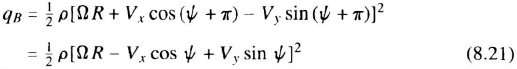
where

Ω	is the rotation rate of sensor in rad/sec
R	is the radius arm
Ψ	is the rotation angle of sensor with respect to reference frame = Ωt

Figure 8.9 Geometric relationships for rotating anemometer sensor.

Solving for q_A − q_B yields

Thus, the pressure difference, q_A − q_B, is proportional to the port speed ΩR of the rotating probe. If V_x = 1.0 ft/sec and V_y = 0, the pressure seen by the transducer at sea level (ρ = ρ₀) will be magnified significantly over what would be seen by a conventional pitot tube. For example, if R = 0.5 ft, Ω = 12 rev/sec = 24π rad/sec, and V = 1.0 ft/sec, then for the rotating sensor,

and for a pitot tube,

The amplification obtained by rotation is therefore 0.179/0.00119 = 150.

In addition to obtaining improved sensitivity at low speeds, the rotating probe measures omnidirectional airspeed, including backward velocities. V_x and V_y are extracted from Equation 8.22, which then permits true airspeed V_t and sideslip angle β, to be obtained using the relationships

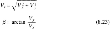
The rotation axis is assumed to be near vertical so, at large bank angles, the V_x and V_y measurements are no longer accurate, and the solution is ignored. In level flight, V_x and V_y are used to estimate the wind vector which is important in fire control equations. Figure 8.10 illustrates an internal view of a rotating anemometer sensor.

Vortex Sensing The sensor measures vortices shed by fluid flow over a deliberately-inserted obstruction. The frequency of vortices is proportional to the air speed. This method has been used to measure low airspeed in helicopters and in ground-vehicle fire-control systems [1, 17, 46]. A version was used on early models of the AH-64D aircraft.

The theory of the vortex sensor dates back to Von Karman in about 1912 [41, 19]. The frequency F of vortex formation from each side of the obstruction is given by

Figure 8.10 Omnidirectional airspeed sensor, rotating anemometer type (courtesy, Pacer Systems, Inc.).

where S is the Strouhal number, V is the air velocity, and d is the width of the obstruction. The Strouhal number has been experimentally determined for a variety of obstruction widths and fluid properties [35]. Theory and experimental work have shown that the sensitivity threshold for this type of sensor is about 1.0 knot. One method of measuring vortex frequency directs an ultrasonic beam through the vortex trail. The rotational velocity of the vortices combine vecto-rially with the sonic ray velocity, causing the sonic rays to be deflected. This causes an amplitude modulation of the received energy at the vortex frequency. To measure the horizontal velocity vector, an orthogonal sensor is required. As in all helicopters, the airspeed sensors should be mounted above the rotor for minimum downwash effects.

Swiveling Pitot Tube Below Rotor The swiveling pitot tube was developed in the United Kingdom; it is currently in use on the AH-1S, AH-64D, and other attack helicopters. It was tested extensively by the United States Army in the 1970s [15, 16, 45]. A gimballed pitot tube contains a vane arrangement that causes the tube to align with the airflow within the downwash field emanating from the rotor blades. Changes in the airflow field vector are correlated with changes in true airspeed. With appropriate angular pick-offs to measure vane orientation, the true airspeed is estimated using a calibration associated with each aircraft and its rotor system.

The theory of its operation can be seen in Figure 8.11 for low-speed, forward flight. The induced flow velocity, V_i is normal to the rotor tip path plane. V_i sin i is proportional to the thrust component that overcomes aircraft drag and causes a forward velocity. The vector diagram is expressed by

A swiveling probe aligns with the resultant flow velocity V, sensing both its magnitude and angle, α and β. The principle of the probe is that V_i sin i is a repeatable function of horizonal airspeed, irrespective of thrust, weight, vertical speed, sideslip angle, center of gravity, but varies only with ground proximity. Hence, a radar altimeter measurement is required to accommodate the ground effect. The basic sensing equations are

Figure 8.11 Flow field vectors for swiveling probe.

where β is the yaw angle also measured by the swiveling probe. Placing a pitot tube in the downwash flow field avoids the need to measure the low pressures existing near hover since the minimum downwash airflow V_i will always be greater than about 15 knots. Also, aligning the pitot tube with the airflow eliminates alignment errors in both the pitot and static pressures. Figure 8.12 is a cutaway view of the swiveling probe.

Analytical Estimation of True Airspeed A predictable airspeed vector results from each combination of collective and cyclic control trim position, and pitch and roll attitude. Methods have been developed [6, 31] that estimate a helicopter's airspeed vector from measurements of these quantities. Augmenting these estimates with inertial velocity accommodates dynamic, nontrim conditions. Flight tests have demonstrated accuracies of 4 knots, 2-sigma using this approach [6].

8.5.2 Optical Air-Data Systems

Laser Velocimetry Nonintrusive optical methods of flow visualization have been part of wind tunnel test instrumentation [7, 25]. Since the 1970s, optical techniques have also emerged as viable air-data systems, motivated by the radar-observability penalty of intrusive probes and by the unsuitability of intrusive probes for hypersonic flight. Optical sensors are located within the vehicles and look out through the local flow into the free stream. Laser velocimeters that measure the Doppler shift from backscatter of naturally occurring aerosol particles have been tested on aircraft since the 1970s in experiments related to the detection of clear air turbulence. Laser radars (Lidars) have also been used experimentally to detect microbursts and severe wind shears. During the 1980s and early 1990s, several laser velocimeters were marketed to calibrate intrusive air-data systems; NASA has experimented with them for hypersonic applications [7].

The basic concept of the laser velocimeter is illustrated in Figure 8.13, a one-dimensional view of the system geometry. In most applications, three orthogonal sensors are used in which the laser beam is split into three component beams. Each is focused at a standoff distance sufficiently removed from the aircraft to be in undisturbed flow (typically several meters away). The lens configurations that converge the beams, with optimum polarization and geometric characteristics for maximizing backscatter response, are generally proprietary with suppliers of such systems.

Figure 8.12 Airspeed and direction sensor, swiveling probe (courtesy, GEC Avionics).

The reflected or “backscattered” signal is Doppler shifted from the transmitted frequency by an amount proportional to the relative velocity between the aircraft and the undisturbed atmosphere. Backscattered signals are mixed with the transmitted signals using interferometers. Test results show accuracies of one knot or better at altitudes where particle (aerosol) density is adequate. Aerosol densities and particle sizes vary with altitude, time, and volcanic eruptions. Testing has shown that there is adequate aerosol density up to about 10,000 meters. Blending the inertial velocity vector with an optically derived true airspeed vector allows operation at higher altitudes.

In 1996, laser velocimeters met the civil and military eye-safety standards, although there may be some question regarding the intensity at the focused region. The trend is toward improved signal processing and lower-power laser beams.

Figure 8.13 Laser Doppler velocimeter.

Particle Time-of-Flight Method Another laser-based airspeed-measurement technique estimates the time of flight required for aerosol particles to traverse the distance between two laser beams, Figure 8.14. Two sheets of laser light, separated by a distance d of a few centimeters, are transmitted through a window in the aircraft's skin. The light sheets are in the YZ-plane, so they measure V_x. Airborne particles generate signals in each of the two detectors that can be timed or correlated; hence true airspeed can be determined.

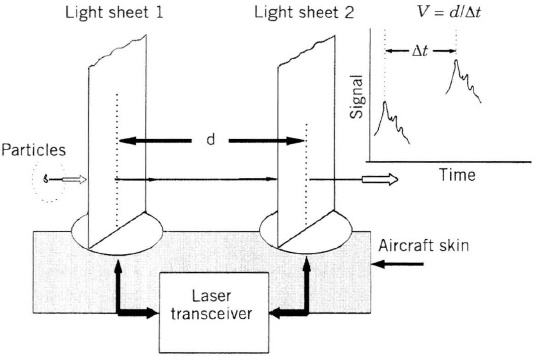
Figure 8.14 Particle time-of-flight method of measuring airspeed.

Figure 8.15 Flush-mounted air-data system with distributed pressure ports.

Bogue [7] has reported good performance on an F-104 aircraft. In addition to particle reflections, the detector sees ambient radiation from sky or ground. Thus, selection of laser wave length, optical filters, and signal-processing are difficult design issues. A successful product would have to measure particles penetrating the light sheets at a distance of 5 to 10 meters from the aircraft skin. Figure 8.15 shows one axis.

Altitude Measurement In conventional air-data systems, altitude and air density are derived from the static pressure measurement. Optical air-data techniques have not demonstrated any methods that will measure pressure, but there are approaches to measuring density ρ and temperature T from which pressure p can be inferred (Equation 8.10). Bogue [7] describes test results with a fluorescence and Rayleigh scatter sensor. In 1996, performance was not adequate for measuring pressure altitude.

8.5.3 Hypersonic Air Data

Air-data measurements in hypersonic flight do not provide primary flight control parameters. They usually support aerodynamic research to confirm structural loading and aero-thermal models. In controlling air-breathing engines (scramjets) in hypersonic flight, pressure and flow-direction measurements are critical [20]. From the earliest experiences with hypersonic vehicles, it was recognized that conventional air-data measurements would be inadequate, primarily because of the thermal loads and shock wave effects on pitot tubes and vanes. Nonintrusive probes were studied in the early days of space flight [40]. The X-15 research aircraft, which flew to 350K ft and Mach 6.7, used a servoed nose ball and conventional pressure transducers [42, 44, 20].

In the X-15, a spherical ball (Q ball) was located in the forward part of the aircraft's conic nose. The ball was servo controlled with hydraulic actuators to align with the relative wind by nulling differential pressures derived from pairs of lateral and vertical pressure ports on the ball. The ball's rotation measured angles of attack and sideslip. Flush-mounted static pressure ports were located at the side of the conic nose. Performance of the ball was adequate to monitor hypersonic and supersonic flight. Nevertheless, the X-15 was augmented with conventional pitot-static probes for subsonic flight and landing. Mach accuracy was 5% to 10%, becoming worse at the low total pressures existing at its peak altitude.

The Space Shuttle Orbiter does not use an air-data system during launch or reentry. It deploys conventional pitot tubes when it has slowed to about Mach 4.0. A variation of the ball nose sensor is used in the Shuttle Orbiter's shuttle entry air-data system (SEADS), where an array of flush pressure orifices are distributed around the nose section [20, 38, 43]. This array includes 14 orifices on the nose cap and 6 aft of the nose cap. Figure 8.15 illustrates the concept of locating multiple pressure ports around an aircraft forebody to extract total pressure and flow direction. This type of configuration is also referred to as a flush air-data system (FADS) and has been used at NASA Dryden in high angle-of-attack research flights [7]. In general, the differences in pressure between upper and lower orifices measure angle of attack and the differences between left and right orifices measure sideslip angle. Algorithms that combine all sensors to determine total pressure are refined during wind tunnel testing. In-flight determination of α and β with SEADS has been accurate to about 0.25 degree; P_t has been accurate to 0.5%. However, static pressure remains the largest source of error which results in a Mach number accuracy of about ±5% [20, 38].

8.6 CALIBRATION AND SYSTEM TEST

8.6.1 Ground Calibration

Typical equipment used to calibrate both the sensors and the central air-data computers is shown in Figure 8.16. The elements in this figure are usually part of automatic test equipment (ATE), with the pressure sources packaged in a separate pneumatic test module. Manometers are the most precise way to measure the pressures that are applied to sensors, but most test sets use secondary standards, often a specially calibrated version of the sensor used in the flight equipment (“unit under test”). Pressure measurements with an accuracy of 0.005 in. of H_g (0.127 mm of H_g = 0.17 mbars) are required.

When calibrating a sensor, the valves shown in Figure 8.16 would respond to test software that commands the pneumatic test module to produce a sequence of input pressures. The sensor outputs are fed to a test computer (“monitor of displays and outputs” on the figure), compared against stored values, and recorded. At the factory, the sensor is mounted inside a temperature chamber, and the pressure test sequences are applied for various temperatures. The result is a table of errors versus pressure for each test temperature. These tables are stored in a calibration ROM that is mounted on the transducer or in the computer.

When the unit under test is a complete air-data computer, the ATE applies a sequence of pressure inputs corresponding to discrete values of altitude, airspeed, and Mach. It also sets simulated temperature-probe resistances and angle of attack to specified values. The output of the computer, usually in the form of a serial digital word stream, is read by the ATE. A dynamic test is also run in which a continuously changing pressure sequence is applied corresponding to a flight profile. The performance capability of the pneumatic test module often limits the severity of the test dynamics.

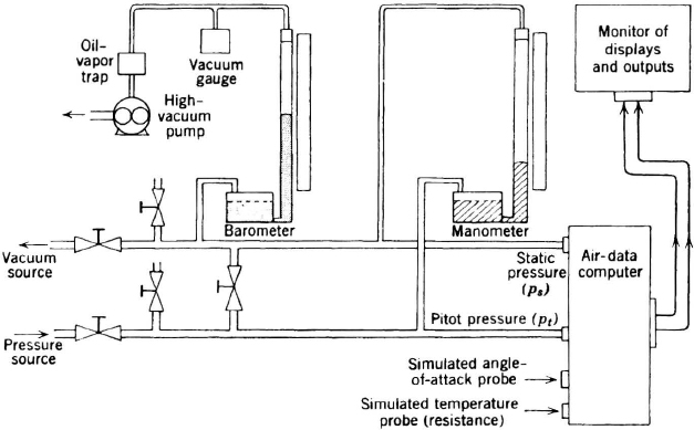
Figure 8.16 Typical test and calibration system.

8.6.2 Flight Calibration

Flight calibration is often a limit to the attainable system accuracy. To calibrate for static defect and for local flow corrections to α vanes, test aircraft are usually equipped with booms that extend forward of the aircraft's nose (Section 8.2.1). These booms contain specially calibrated pitot static tubes and flow direction vanes. On-board laser velocimeters have been used to augment this process (Section 8.5.2). With contemporary inertial/differential-GPS systems, precise aircraft ground velocity is also available.

8.6.3 Built-in Test (BIT)

Digital air-data systems can detect nearly 100% of their own failures. At startup, processor tests and memory tests verify computer operation. Continuous BIT checks all interfaces, “wraps around” outputs into inputs to check A/D and D/A conversions, and verifies that the processors are operating properly. BIT monitors a sensor's function such as excitation voltages and oscillator or voltage reasonableness. However, it cannot detect a slow degradation of accuracy resulting from a mechanical deterioration of a sensor (e.g., a leak in the tubing). Since air-data functions are often critical to flight safety, systems are redundant. Thus, transport aircraft use dual or triplex air-data systems. Combat aircraft often use single air-data computers but provide pneumatic altimeters and airspeed indicators as backup.

8.7 FUTURE TRENDS

With the growing popularity of distributed architectures in which redundant “smart probes” incorporate processors, the CADC is disappearing and flight-control, navigation and flight-management computers are executing the air-data computations. Optical air data measurements offer attractive solutions for difficult applications where intrusive probes are precluded. Micro-machined transducers are likely to come into widespread use. The size and cost of electronics are being steadily reduced by new computer and input-output chips.

PROBLEMS

8.1. (a) At an altitude of 20,000 meters (65,617 ft), the static pressure measurement is 41.41 mm of Hg, What is the static temperature?

(b) If Mach number is 4.0 at this altitude, what is the impact pressure q_c in mm of Hg?

(c) Under the above conditions, what is the true airspeed in knots?

Ans.: (a) 235 K; (b) 831 mm Hg; (c) 2388 knots.

8.2. (a) If an aircraft is flying at Mach = 0.8, what is the impact pressure to static pressure ratio q_c/p_s?

(b) If the aircraft has an uncorrected static source error of ±5% and a pitot tube error of ±5%, what is the range of computed Mach numbers?

Ans.: (a) q_c/p_s = 0.524; (b) M = 0.766 to 0.835.

8.3. (a) A digital autopilot is to maintain altitude to an accuracy of 0.5 meters. Its spec calls for a resolution of 5.0 cm. The aircraft has an altitude ceiling of 20,000 meters. To meet the specification, how many bits are required to encode the altitude measurement?

(b) To meet the 5-cm resolution, what pressure measurement sensitivity will be required for the static pressure transducer?

(c) What is wrong with this specification?

8.4 At what airspeed will a conventional pitot tube become more sensitive than a rotating anemometer type of airspeed sensor and at what speed will the pressure at the pitot tube transducer exceed the pressure measured by a rotating anemometer?