The current ratio (and its close cousin, the quick ratio) is one measure of a company's ability to meet its short term obligations. Creditors and potential creditors typically pay attention to the current ratio because it tells them if the company is in a position to pay off its liabilities with assets that it can quickly access.

The definition of the current ratio is:

(Current Assets) / (Current Liabilities)

Current assets are usually defined as those that can be converted to cash within a year, and current liabilities are obligations that come due within a year. So, if a company has a current ratio of 3, it can pay its known liabilities three times over from existing, relatively liquid resources. A current ratio of 3 would tend to be regarded as fairly high — a current ratio of 2 or more is usually considered satisfactory by creditors.

But a company's current ratio can be too high, even though the higher the current ratio, the better creditors like it. When too much of a company's resources are in current assets (cash, accounts receivable, inventory, and prepaid expenses usually account for most of a company's current assets), it may be that the resources are not being invested to the company's best advantage. Having $30,000 in a cash account does not tend to support the creation of new revenue; having $30,000 invested in a new delivery van does.

It's usually a good idea to look at a company's current ratio along with a closely related measure, working capital. The current ratio is the ratio of current assets to current liabilities, whereas working capital is the result of subtracting current liabilities from current assets. Chapter 5 has much more to say about working capital. For the moment, consider two companies, one with current assets of $30,000 and current liabilities of $10,000, and one with current assets of $300,000 and current liabilities of $100,000. Both have current ratios of 3. But the first company's working capital is $10,000 while the second company has $200,000 in working capital. Clearly, the second company will have a much easier time qualifying for a loan than the first company.

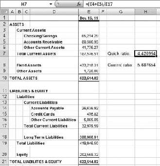
QuickBooks' Summary Balance Sheet report is the easiest way to get the current ratio (as well as the quick ratio, explained in the next section). To get the report, choose Reports

Figure 6.1. The current ratio based on these figures is probably much too high for management's comfort.

Once you've pulled up this report, you can tell the company's current ratio, at least roughly, with just a glance at the total current assets and the total current liabilities. In the figure it's between 5 and 6, which is unusually high, and a large fraction of the current assets is in accounts receivable. If you were a creditor, you'd take comfort in these figures, but if you were a stockholder you might want less liquidity and more investment in the company's future — something should be done with that $155,000 in working capital. And if you were a manager in the company, you'd probably want to look at the company's average collection period (see the final section in this chapter).

The quick ratio, sometimes called the acid test, takes an even more conservative look at a company's liquidity than does the current ratio. The idea is that some current assets are more current than others. In particular, it takes longer to convert inventory to cash than to convert receivables; the same is true of prepaid expenses, some of which may not be convertible to cash at all. Cash is cash, of course, and the company can press for payment of receivables if necessary.

Some analysts therefore want to look at the quick ratio as well as the current ratio. The quick ratio subtracts inventory from current assets in the ratio's numerator. Formally:

Quick ratio = (Current Assets – Inventory) / (Current liabilities)

In Figure 6.1 you can see that the company's quick ratio is between 4 and 5: about $146,000 in cash and receivables, and about $33,000 in current liabilities.

As with the current ratio and working capital, it can help to evaluate the quick ratio in the context of another figure, the average collection period (again, see the final section in this chapter). If the length of time that the company has to pay its vendors is roughly the same as its average collection period, then payment and receipt schedules are in line with one another and a quick ratio of 1 is acceptable.

But if it takes a company 60 days or longer, on average, to collect its receivables and its vendors are pressing for net 30, there might be much less liquidity than a quick ratio of 1 would normally suggest.

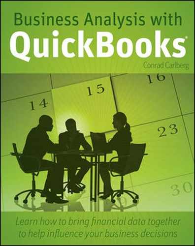
If you don't feel like glancing at the balance sheet and doing the addition and division mentally, just click the report's Export button and move the data to an Excel workbook. There you can compute both the current ratio and the quick ratio directly, as shown in Figure 6.2.

Figure 6.2. You can calculate a variety of financial ratios directly from the Balance Sheet Summary report.

As a manager, and possibly the owner, of a company that seeks to conduct its operations without actually losing money, you know that you have more control over how the company spends its money than you do over how your customers spend their money. Much of your time goes to making sure that expenses are under control and, where possible, staying focused on creating more revenue.

One indicator that's useful in the control of expenses is the operating expense ratio, particularly when you view it across more than one accounting period using a comparative P&L. Figure 6.3 shows a comparative P&L summary. To obtain it, choose Reports

At first glance, this report looks like good news: Sales are up over 27% year to year. But the bad news immediately sets in when you look at the cost and expense categories. The COGS is up over 33%, and gross profit must fall when COGS rises more than sales. This can happen when a company reduces its sales price, usually in an effort to increase volume, but its vendors hold the line or even increase their pricing.

Then the General and Administrative (G&A) expenses have increased, also more than sales, so they are eating up more of the gross profit during the second year than they did during the first. It is particularly troubling when G&A rises faster than sales. Although some G&A costs rise and fall in line with sales (bonuses, for example), many administrative costs such as office space leases are fixed or, perhaps, semi-variable. So you generally expect to see G&A costs rising slower than sales, not faster.

You would have to look further than a P&L allows to determine the reasons that sales expenses rose nearly two-thirds when sales rose less than one-third. It's possible that in trying to increase sales, commissions were boosted, or there was more travel. Whatever the reason, it did not pay off, at least not so far, with a commensurate increase in revenues.

As an owner or manager, it's not sufficient that you pursue increased revenue. You want to pursue profitable revenue. And when operating expenses are rising faster than sales, as is the case in this example with G&A and sales expenses, you need to investigate the reasons. It could easily be due to something reasonable and one-time, such as additional office space to accommo date new staff. But if it's due to things such as a $1,400 wastebasket for the CEO, then there are problems looming that had better be corrected before the costs outstrip the sales.

Figure 6.3. The Percent Change in QuickBooks' comparative reports use the earlier period's value as the denominator.

It does help to focus on the expenses where you have more, or more immediate, control, and the operating expense ratio can tell you if you need to delve further. The ratio is defined simply as follows:

(Operating Expenses) / (Net Sales)

In this example, for the year 2010, the ratio is 115,600 to 510,000, or 22.7%. For the year 2011, it's 174, 960 to 648,000, or 27.0%. That may not seem like too much, a difference of 4.3%, but if operating expenses just kept pace with sales in 2011, then net income would have grown 15.6% instead of falling by 11.8%. Figure 6.4 shows that analysis. The reports are exported to Excel for more effective comparison.

Figure 6.4. Comparative income statements with rising, and with constant, operating expense ratios

In Figure 6.4, columns B, C, and E show the comparative P&L data from the QuickBooks report in Figure 6.3. The total operating expenses increase by 51.3% from 2010 to 2011 (cell E9) as net sales are rising 27.1% (cell E2). The result is that net income falls by 11.8% (cell E17).

Now look at columns G, H, and J. The only differences are in operating expenses in rows 7 through 9, which have been constrained in 2011 to the same rate of change (27.1%) as net sales in row 2. Because the expenses are lower, the income tax for 2011 is higher than it was when the operating expenses were greater (compare cells B16 and G16). And yet, even with an additional $11,284 in income taxes, the company's percent change in net income rose from −11.8% to 15.6%.

Notice also that the operating expense ratios in cells G20 and H20 are identical, whereas the ratio increases by 4.3%, as noted in the figure, in cells B20 and C20.

The concept of the return on assets (ROA) is fundamental to an assessment of how well a company's management is handling its resources. Conceptually, ROA is a measure of the income earned, adjusted for the amount of assets available to support the earnings process. More objectively, it is defined as follows:

(Net Income) / (Total Assets)

If you have $1,000 available in the form of assets — cash, equipment, supplies — and you create $100 by using those assets, your ROA is 10%. If you manage the $1,000 in assets a little more effectively and create $140 in net income, your ROA is a slightly more robust 14%.

Calculating ROA

More specifically yet, the "net income" that's the numerator in the ROA ratio usually has interest payments added back in. The reason is that the net income calculation subtracts COGS, salaries, supplies, and other costs from gross profit. Among those other costs are interest payments on loans taken out to increase the company's total assets. The cost of acquiring the assets that are to be managed should not count against the manager's effectiveness in generating income with those assets. Therefore interest payments are added back in to net income before calculating the ROA.

Bear in mind that the P&L shows the accumulation of income and expenses over time: for example, the current year to date, or current quarter, or some other time span that's important to you. The balance sheet, in contrast, represents a snapshot, the amount of money that the company has invested in different accounts and that it owes in the form of various liabilities, as of the report date. It's a good idea, therefore, to get a measure of the company's total assets over the full period of time covered by the P&L. One way to do that is to take the average of the total assets at the beginning of the period and at the end of the period.

Figure 6.5 shows a variation of the balance sheet in Figure 6.1. Figure 6.5 shows a comparative balance sheet, one that makes it easy to compare account balances on December 15, 2011, with those from exactly one year earlier. With the total assets at the beginning and at the end of the period in view, it's easy to average them for a slightly more accurate ROA estimate.

To get the sort of comparative statement shown in Figure 6.5, take these steps:

1. Open a Balance Sheet Summary report by choosing Reports

   

2. Click Modify Report. The Display tab appears as shown in Figure 6.6.

3. Fill the Previous Year checkbox and click OK.

Using the average of the start and end of the period as an estimate of total assets is better than a single-date snapshot, but it's still a relatively crude estimate and it's a relic of times when a balance sheet as of any given date could not be quickly and easily obtained. If you're concerned about getting a more accurate estimate of the typical level of total assets during, say, a year of the company's operations, you can get it for each month and then take the average across 12 evenly-spaced dates, not just two.

To do so, first refer back to Figure 6.6. Instead of filling the Previous Year checkbox in the Modify Report dialog box, use the Display Columns By dropdown at the top of the report itself and choose Month. Then, after you click OK, the report will appear as shown in Figure 6.7.

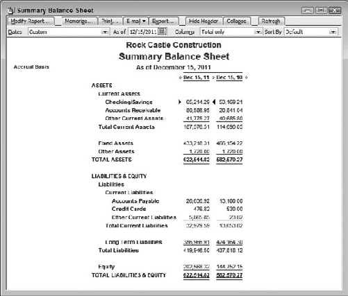
Figure 6.5. By tradition, comparative statements show the more recent accounting periods on the left.

Figure 6.6. You can choose a range of dates, but the results are shown for only the ending date.

Figure 6.7. You can't see it here, but the columns extend through December 15, 2011.

Of course it's a lot more difficult to take the average of 12 asset values in your head than just two, so it's a good idea to export this report to an Excel workbook and then compute the average.

The corresponding P&L appears in Figure 6.8. Notice that it covers the period from December 15, 2010, through December 15, 2011.

Only a portion of the P&L is shown in Figure 6.8. Notice that an Expand button appears at the top of the report. This button is a toggle. If it were clicked, subaccounts would appear in the report and the button's caption would change from Expand to Collapse. With the report collapsed, the user can see that interest expense for the period shown is $2,217.31. Adding interest back in to net income results in $57,816.17 + $2,217.31, or $60,033.48.

Using the data from Figure 6.5, the average total assets at the beginning and end of the 12-month period is $602,542.55. The ROA is therefore $60,033.48 ÷ $602,542.55, or almost exactly 10%. Is that good, bad, or indifferent? The ROA from other, similar companies — a type of vertical analysis — can help determine whether the company is operating more or less efficiently than its competitors. It can also be useful to compute the ROA on the same company but from other years — a horizontal analysis that can help determine whether a company is operating more or less efficiently over time.

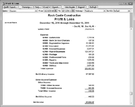
Figure 6.8. The custom report dates are chosen to align the data more closely with the report in Figure 6.7.

=(1+ RATE(24,-2710.90,60000))^12-1

The Balance Sheet Summary, shown in Figure 6.1, and in worksheet format in Figure 6.2, make it very easy to determine the company's equity ratio:

(Total Equity) / (Total Assets)

Just divide the value in cell E20 of Figure 6.2 (the company's total equity) by the value in cell E10 (the company's total assets). In this case that's $202,568.32 divided by $622,514.82, or 33%.

If you hold stock in this company, you should watch its ROA carefully. A low equity ratio (and 33% is rather low) shows that the company has acquired most of its assets through borrowing rather than by using its equity. As described in the earlier section on ROA, leverage magnifies the effect of borrowing, whether that's good or bad. If the ROA is less than the rate paid to service the debt, the degree of leverage accelerates the loss. And the equity ratio is one measure of the amount of leverage the company is using.

The danger to the company becomes more apparent when you put yourself in the position of a stockholder. The company has in this example financed two-thirds of its assets through borrowing. If the return on those assets is less than the company is paying to finance the debt, then your return in the form of dividends or stock price also suffers. You could do better by lending the company money than you can by investing your funds in it.

The combination of a low equity ratio (therefore, high leverage) and a relatively poor ROA would pressure you, as a stockholder, to sell your stock if feasible. So will other stockholders. And that makes it very difficult for the company to raise money in the capital markets.

On the other hand, if the ROA is greater than the debt service, you can do better as an investor than you can as a creditor. The lesson is that if the company has a relatively low equity ratio, an investor needs to watch its ROA and its debt service.

As mentioned in the prior section, the debt ratio is the complement of the equity ratio. You can find it either by subtracting the equity ratio, calculated earlier, from 1.0, or directly by the formula

(Total Liabilities) / (Total Assets)

In Figure 6.2, that's cell E19 divided by cell E10, or 67%.

If you were a creditor you'd prefer to see a debt ratio that's a lot closer to 33% than 67%. Suppose that the company loses value precipitously and must liquidate its assets. The assets themselves then lose value, and a high debt ratio suggests there might not be enough in the way of devalued assets to pay off all the creditors. A low debt ratio, and a correspondingly high equity ratio, provides more protection to creditors against a reduction in the company's asset value.

The ratio called "times interest earned" can be considered a leverage ratio because it depends in part on the amount of debt service a company must pay during an accounting period, typically a year. But while the debt ratio looks at total liabilities as a fraction of total assets, the times interest earned ratio looks at the cost of the debt as a fraction of income.

Creditors are of course vitally interested in a company's ability to repay the principal of a loan, but they also want to know to what degree the company is positioned to make its periodic interest payments. That ability is measured by the ratio of income to interest payments, or the multiple of the interest that is represented by income: the number of times that the interest is earned.

The divisor in the ratio is simply the dollars in interest payable during the year. The numerator is the company's operating income, with a couple of adjustments. The income should be before interest and income taxes are deducted to arrive at net income — that is, EBIT, or earnings before interest and taxes. The rationale is that the analyst wants to know how much money is available for interest payments, and therefore those payments should not be subtracted in arriving at the income estimate. Furthermore, because the income tax amounts depend on the deductible interest amounts, they should not be subtracted from the income.

Figure 6.9. In a closer case, you should probably export the data to Excel for the calculations.

Each value, the interest payments and the pre-interest, pre-tax income can be found on, or easily derived from, the P&L Standard report (see Figure 6.9).

The example in Figure 6.9 clearly returns a very large times interest earned ratio — large enough that you can quickly see that there's no problem lending this company some money. In a closer case, such as a company with a much smaller ratio of EBIT to interest payments, let Excel do the calculations for you. The times interest earned ratio often ranges from 2 to 6, and a ratio between 3 and 4 is typical. Ratios in the 3 and 4 range are strong enough to encourage lending.

The inventory turns ratio, sometimes called the inventory turnover ratio, is an indictor of how well a company manages its investment in merchandise, whether at the wholesale or the retail level.

You may have come across the term just-in-time inventory. It refers both to a goal and to procedures that are meant to help meet the goal: to bring goods into inventory no sooner than needed for manufacture, or onto a reseller's shelves no sooner than needed to support revenues. The idea is that the longer a company owns goods, the longer its financial resources are tied up in a static investment and are unavailable to create more profit.

The sales/week ratio

In QuickBooks, when you set up a new inventory item — or when you edit an existing item — you might supply a reorder point on the item record. (Choose Lists

Regardless of how you come up with a reorder point, it represents one way to express the idea of a turns ratio. A rational reorder point takes into account how soon you need more of an item and how long it will take your supplier to fulfill your order. If you sell 20 units a week, and if your supplier needs two weeks' lead time, then you should probably reorder when you're down to 40 units in stock.

The phrase "20 units a week" in the preceding sentence is a measure of inventory turns: an inventory level of 20 turns over once a week. But that's too specific a usage. Instead, it's usual to talk in terms of an annual turnover rate, and to generalize the ratio to a dollar value: cost of goods sold, or COGS.

The turns ratio

Before cheap computing power became broadly available, the turns ratio was often calculated in this way:

(Annual COGS) / (Average Inventory Asset Value)

where the average inventory level was just the inventory value at the start of the year plus the inventory level at the end of the year, divided by 2.

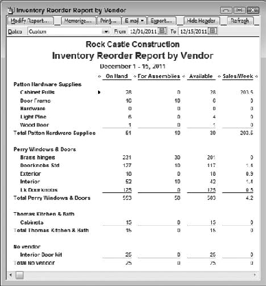
Figure 6.10. The sales/week ratio in the final column is a measure of units sold, not dollars reinvested.

There are problems with that approach. For one thing, companies often arrange their inventory levels to be lowest on the date their fiscal year's start (and end). This is to dress up their financial statements, so it will not appear as though their resources are tied up in stock sitting on shelves, but hard at work generating new profits. Therefore, the average inventory level is often an underestimation of the actual level throughout the year, and the turns ratio was therefore not representative of the actual inventory activity.

Notice that this ratio is calculated in terms of dollars: the cost of goods sold, divided by a measure of typical inventory value. This is handy, because by using a ratio of dollars to dollars it's possible to compare turns ratios across items, or product lines, or even companies. To see the advantage of working with ratios based on currency units, consider the QuickBooks Inventory Reorder Report by Vendor (see Figure 6.10). This report is found in the Premier Manufacturing and Wholesale edition of QuickBooks, but don't worry if you don't use it — my mentioning it is meant only to illustrate why your management decisions should look beyond simple unit counts.

The sales/week ratio shown in Figure 6.10 is a helpful number from the perspective of ordering new inventory from the supplier. You can see, among other fields, how many units you have on hand, how many are committed, how many are available, and how many you have sold per week during the report's time frame. Operationally, the sales/week ratio can be a very useful number because it tells you if you're likely to run out of product in the near future.

Figure 6.11. The Inventory Valuation Summary report helps you build up a rough estimate of average inventory levels.

But from a business analysis or a management perspective, it's not so useful. Suppose your purpose in looking at inventory status is not to decide when and if to buy more goods, but whether or not a product line moves well enough to justify retaining it in your business mix. Selling cabinet pulls at a 250 per week clip is all well and good, but that number by itself does not address an important issue: How long does it take to deplete your existing stock at that run rate?

That's what the turns ratio is intended to examine. Figure 6.11 shows two Inventory Valuation Summary reports for Rock Castle Construction, for the first and last days of 2011. No customization is needed to produce this report, other than specifying the date for the summary.

It helps to start with the full inventory analysis as a context. Figure 6.11 shows the overall inventory level on 1/1/2011 was $12,810.15. On 12/31/2011, the inventory level was $28,807.29. The average of the two inventory valuation figures is ($12,810.15 + $28,807.29) ÷ 2 = $20,808.72, a fairly crude but not irrational estimate of how much the company has invested in its inventory on any given day.

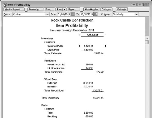
Figure 6.12. Be careful to pick up the total cost for inventory, not the grand total cost which might include non-inventory parts.

Figure 6.12 uses the Item Profitability report to get a COGS figure for the overall inventory during the same period of 12/1/2011 through 12/15/2011. This report has been modified, using the Modify Report button, to show only the Actual Cost column, and to use 1/1/2011 and 12/31/2011 as its starting and ending dates. To display the Item Profitability Summary, choose Reports

The company used $16,373.14 — the COGS — in inventory during the time period in question. So, an estimate of the turns ratio for the company's overall inventory is $16,373.14 ÷ $20,808.72, or almost exactly 0.8. Overall, during the 12 months of 2011, this company runs through 0.8, or 80%, of its inventory. The stock turns over 0.8 times per year.

With that figure as context, here's a look at a particular inventory item. In addition to the overall inventory, Figures 6.11 and 6.12 show the required data for Rock Castle's supply of exterior wooden doors. With a starting inventory of $210.00 and an ending inventory of $4,374.05, the average is $2,292.03. Combined with COGS of $11,049.14, the resulting turns ratio is 4.8. That is, the company's average supply of exterior wood doors turns over not quite five times in 2011. Clearly, some other inventory item or set of items is selling so slowly that it's dragging down the company's overall turns ratio. Only a similar examination of the other inventory items will identify the source of the problem.

And it is a problem. Inventory is traditionally and conventionally regarded as a current asset, and the usual definition of a current asset is one that can be converted into cash within a year. This company's inventory is turning over — being converted to cash — less than once a year. Once every 15 months, to be precise. That's not good enough, and if you were the company's owner you would demand to know why you're carrying so much stock, or selling it so slowly, that your overall inventory turns ratio is only 0.8.

There are some other issues to keep in mind with the turns ratio, as the following subsections explain.

Average inventory

Two factors can cause a low turns ratio: a low COGS and a high inventory level. If your company has done its account setup and data entry properly, it's hard to argue with the figure that QuickBooks gives you for COGS. But the average inventory level is another matter.

Earlier in this section, I mentioned that the average of the inventory at the start and the end of the fiscal year might be misleading, because companies sometimes manage to time their fiscal years with periods of low inventory. If you're going to go to the trouble of getting a starting and an ending inventory, you might as well do a little bit of additional work and get the starting inventory for each quarter as well as the end of year level. Add them up and divide by 5 to give you a better estimate of the actual average inventory level. You can go further and get monthly figures to average, as explained later in the "Average collection period" section.

Best would be to determine the asset value in stock for each day during the fiscal year. That's feasible, but it requires exporting the inventory valuation detail report to Excel and then doing some hand-waving to get a value for every calendar day, not just those days on which a transaction occurs. If you do this, bear in mind that any day that has no activity for a given item carries the same total asset value as the most recent day on which a transaction involving that item occurred.

High turns

A high turns ratio is usually regarded as a positive sign, but if it's high compared to similar companies there may be a problem. Because part of the ratio is some measure of average stock level, a high ratio can be due more to low stock levels than to high sales. Low stock levels can mean that some customers are turned away or otherwise underserved because the company maintains insufficient stock levels. I mention this only because this point is frequently cited. It actually occurs less frequently than the number of citations suggests.

Relationship to gross profit rate

It often happens that high inventory turns rates are found in companies with low gross profit margins. It's not necessarily cause-and-effect. Instead, it is often due to the fact that companies with low gross profit margins, companies that deal in commodities, for example, must turn their inventories over rapidly in order to make up for the low profit margins. Otherwise, they will not be able to produce an acceptable return on assets.

Measuring turns in days

Some analysts find it easier to think of stock turnover in terms of number of days worth of stock. If you divide 365 by an annual turns ratio, you have the number of days worth of stock on the shelf. In the example given earlier in this section, a turns ratio of 0.8 divided into 365 results in 456 days: a year and three months. This figure is useful in combination with the average collection period, explained next, to determine the length of a company's operating cycle.

The average collection period is analogous to inventory turnover. Inventory turnover analysis tells you how long it takes to deplete your stock of goods, while the average collection period gives you a rough idea of how long it takes to collect money for sales made on credit. Together, the two figures make up the company's operating cycle: the initial investment in goods, holding the goods in stock until they are sold, collecting from the purchaser, and then reinvesting that money in more goods.

The average collection rate tells you how long proceeds from credit sales sit in accounts receivable. Formally, it is defined by the formula

(Total Sales – Returns – Cash Sales – Credit Card Purchases) /
   (Average Accounts Receivable)

the ratio of net credit sales to an average accounts receivable balance. (In QuickBooks, net credit sales means total invoiced amounts, less returns.) If you have made $500,000 in net credit sales for a year and your average monthly A/R balance was $50,000 during that year, you are turning over — that is, depleting accounts receivable by means of collections — at the rate of 10 times per year. Your average collection period is therefore 36.5 days. It's important to note that the net sales in this context are limited to those made on credit; sales for cash or via credit card result in immediate collection, or at worst the two or three days it takes a credit card processing bureau to credit the company's bank account.

Obviously, the calculation as described is a rough estimate. It depends on the comparison of the sales made during one period with the collection of funds for sales made at other times. There are many ways to calculate an average accounts receivable balance — daily average, weekly average, average of starting and ending balances, and so on — and each returns a different result if your receivables bounce around much. Which they do.

Ideally, the analysis of QuickBooks data would begin with a list of all credit transactions (in effect, transaction types would include invoices and payments only) that associate an invoice date, amount, terms, due date, payment date, and payment amount. Only then would it be possible to create a more sensitive analysis. Greater precision would enable, for example, the analysis of collection periods across different payment terms, such as net 15 versus net 30. But QuickBooks reports do not tie payment transactions to their associated invoices, so a rough estimate is the best that can be done by means of the user interface.

Here's how to get the average collection period using QuickBooks reports. So that you can see everything in Figures 6.13 through 6.15, the following instructions pick up data by quarter. Remember that when you run your own analysis, you might want more frequent time slices, and pick up the data by month instead of by quarter.

You now have the basis for getting average accounts receivable. It would be useful if you could get net sales on the same report, but from the balance sheet perspective you'll get a cumulative, not a quarterly, figure. To make the analysis easier in Excel it will be best to get the quarterly actuals instead of a running total. So take the earlier seven steps again, with these modifications:

You now have two Excel worksheets in two different workbooks. Suppose that the accounts receivable information is in Excel Book3 and the sales income data is in Book5. They appear in Figure 6.14.

Figure 6.13. Modify the report dates to match your company's particular history.

Figure 6.14. It's a good idea at this point to check that the dates in the two reports correspond.

Figure 6.15. It takes this company an average of 41.2 days to collect on its credit sales.

To complete the analysis, take these steps:

If you have another year's, or more, worth of data, you can repeat Steps 7 through 10 another four columns to the right. Comparison of the annualized data for the two years will tell you whether your average collection period is increasing or decreasing. In turn, that will tell you whether you should take steps to reduce the length of time needed to collect on credit sales, perhaps by adjusting the terms you offer your credit customers.

By adding the average collection period to the inventory turnover period, you can get a measure of how long it takes to turn an investment in goods back into cash. If that length of time is increasing by what is, to you or in your industry, a meaningful amount, that means you are experiencing lower sales and higher investment in inventory. That combination, if left uncor-rected, is sure to hurt your profit.