IN THIS CHAPTER
Exporting Reports to Excel Workbooks
Formatting and Layout Problems
Exporting to Text Files
Analyzing QuickBooks Data with Pivot Tables
To bring a broader array of tools to bear on the data you've entered into QuickBooks, you really need some straightforward ways to make the data available to other applications. Although QuickBooks has various methods you can use to carry out business analysis without leaving its comfortable and familiar user interface, you just can't do it all in QuickBooks. Sometimes you need to send it out.
One method you can use to get data from QuickBooks into another application is the export of a report. To export a QuickBooks report is to make its data available to another application such as Excel. As you'll see in this chapter, the information in a report can be placed in an Excel worksheet where you can analyze the data more fully than is possible in QuickBooks.
The very nature of most QuickBooks reports is to summarize data. Even the detail reports have data summaries that provide totals and subtotals for their detail lines.
The summaries can be helpful because they classify values that otherwise you'd have to deal with yourself: COGS (cost of goods sold) versus office supplies, for example. At the same time the summaries can create problems because they often roll up, and therefore repeat, information already in the report in the form of details. Much of the knowledge needed to analyze business data comes from learning what to keep and what to pitch.
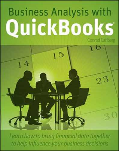
Suppose you want to export an income statement (known to QuickBooks as a Profit & Loss report) from QuickBooks to Excel. There are various reasons you might want to export a report, and perhaps the most typical is so that you can quickly calculate measures such as a Current Ratio or a Times Interest Earned Ratio. Figure 2.1 shows how the QuickBooks report might look.
You start the export process by clicking the Export button at the top of the report. When you do so, the Export Report dialog box shown in Figure 2.2 appears.
The comma-separated values (CSV) option looks like it will take you down a pretty boring road: Saving a report to a simple text file doesn't look nearly as slick as choosing any of the Excel options. But don't ignore the CSV option. Exporting a report in CSV format to a text file can save you plenty of heartburn, especially if you haven't dusted off your Excel skills in a while. See the "Exporting to Text Files" section later in this chapter for more information.
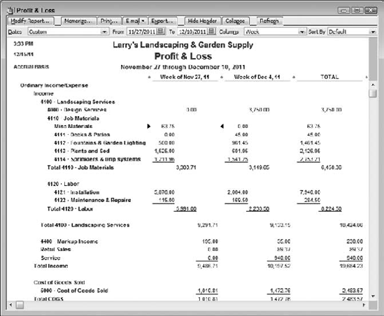

Figure 2.2. There are some traps in the Export Report dialog box. Be sure you understand the effects that the options will have on the exported report.
If you want the report to go directly to Excel, you have two principal choices: a new Excel workbook or an existing workbook. If you export to a new workbook, QuickBooks starts Excel if necessary, establishes a new workbook, and places the report data into it.
Note
The name of the new workbook will be something like Book2, or Book4, or Book6, etc., depending on whether Excel is already open with unsaved workbooks active. New workbooks established by QuickBooks are incremented by 2: Book2, Book4, and so on.
In the Export Report dialog box shown in Figure 2.2, if you export to a new workbook and click OK, your worksheet will look similar to that shown in Figure 2.3, which is based on the report in Figure 2.1.
There are several ways that you might change the worksheet created by the QuickBooks export:
Naming the worksheet
It would be helpful for QuickBooks to give the worksheet the name of the report it is based on, instead of the nondescript default of Sheet1. I urge you to do that yourself, especially if you intend to store additional reports in the same workbook. To rename the worksheet:
Right-click the tab at the bottom of the worksheet. In Figure 2.3, the tab contains the name Sheet1.
Choose Rename from the contextual menu.
The worksheet tab is highlighted. Type a new name and press Enter.
Tip
You can use up to 31 characters in a worksheet name. If you want to name it P&L, I you can do so, but you can't use any of these characters: / ? * : [ ]
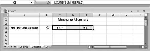
If you're using Excel 2002 (part of Office XP) or later, you might see a mysterious triangle in the upper-left corner of some cells — for example, cell H12 in Figure 2.3. This triangle is a warning that a cell's contents might not be doing what you intend. The warning usually means that the cell contains a formula that doesn't conform precisely to what Excel expects, and so Microsoft wags its finger at you by way of that mysterious triangle.
If you select the cell, a yellow icon with an exclamation point appears next to it. Clicking that icon reveals a menu, headed by a description of what Excel thinks might be an error.
In the case of an exported QuickBooks report, the potential error (1) isn't an error, and (2) almost always means that a formula omits a value in a neighboring cell. Consider cell H12 in Figure 2.3. That cell contains the formula:
=ROUND(SUM(H6:H11),5)
This formula tells Excel to take the sum of the values in cells H6 through H11, round the sum to five decimal places, and display the result in the cell that contains the formula. (Not all five decimals appear because the cell's numeric format is Currency. In Excel, a cell's appearance is normally determined more by its format than by its contents.)
QuickBooks is responsible for putting that formula in H12, and it could have done a slightly better job. This formula's purpose is to show you the sum of the dollars associated with Job Materials subaccounts. Those dollar amounts occupy cells H7 through H11, and the formula should really be:
=ROUND(SUM(H7:H11),5)
As it is, though, Excel notices that cell H5 contains a value, and therefore thinks it is possible that the formula was supposed to include cell H5 in the formula — it's a value in a cell that's adjacent to the cells that the formula sums. So Excel warns you that you might have omitted an important value, and it warns you with that triangle in the upper-left corner of the cell.
You know it's not an error, though, and here are the ways you can deal with the error indicator:
Ignore it.
Select the cell with the error indicator. Click the yellow warning icon and choose Ignore Error from the contextual menu. This removes the indicator from the active cell only.
Select the cell, click the yellow icon, and choose Error Checking Options from the contextual menu. The Excel Options dialog box shown in Figure 2.4 appears. Clear the checkbox labeled Formula Omits Cells in Region and click OK to clear the error indicator, as well as any other instances of the error warning that might be in other cells.
I have been using Excel since the early 1990s, but it still took me around 10 minutes to figure out why a QuickBooks report that I exported to Excel refused to take seriously formulas that I subsequently entered in the worksheet. The following example might save you from wasting the time that I did.
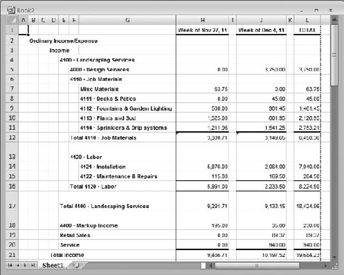
Suppose that you have called for a Profit & Loss Summary report in QuickBooks that has each of two weeks' results in two columns, and their total in a third column. Figure 2.5 shows how the exported report might appear in Excel.
If it's my company, I'd be curious to know how we did in the week leading up to December 4, compared to how we did in the week before November 27. One way to do that is to look at Gross Profit. I'd want to know what percent of the total Gross Profit of $17,200.66 was earned in each of those weeks.
I'd start by entering this formula in cell I25:
=H25/L25

Figure 2.4. To get to the error-checking options in Excel 2007, click the Formulas tab and then click Error Checking in the Formula Auditing group. In earlier versions, choose Tools
expecting it to return a value of something around 50%. I'd be surprised instead to see this in cell I25:
=H25/L25
The cell is not evaluating the formula and displaying its result (actually, 49.3%) but merely displaying the formula itself, as though it were a text value such as Gross Profit.
This is very unusual behavior for Excel, and at first it took a while to solve. When QuickBooks lays out the new worksheet, it gives a Text format to the cells in the print area that contain neither numeric values nor formulas.
You can do the same thing in Excel by right-clicking a cell, choosing Format Cells from the contextual menu, and choosing Text from the Category list box. If you then enter a formula into the active cell, all you will see is the formula, not its result.
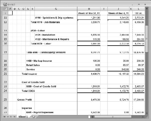
Figure 2.5. You can call for or suppress blank intervening columns via the Advanced tab of QuickBooks' Export Report dialog box.
The way to undo this mischief is to select a column whose cells do not now contain numbers or formulas: for example, column I in Figure 2.5. Right-click the column header, choose Format Cells, choose General from the Category list box (you could also choose Percentage or Number if you prefer) and click OK. Now any formula that you enter in the cell will display as its result. If there's already a formula in the cell, click it in the formula box and either press Enter or click the green checkmark icon, to force it to recalculate.
Skip this section if you consider yourself an experienced Excel user. Otherwise ...
From time to time I see a plaintive question in the QuickBooks user forums from someone who tried to copy an exported report into another worksheet. Usually, that other worksheet is intended as a management report of some sort, and someone wants to add information, exported from QuickBooks, to the report. Then, the added information makes no sense.
Notice in Figure 2.6 that the data is captured starting in row 12 of the exported report. The data is intended to appear in row 3 of the target report. Figure 2.7 shows the result of copying cells H12:J12 in the exported report into cells C3:E3 of the management report.

Figure 2.6. If you want to copy exported QuickBooks data to another Excel worksheet, convert the formulas to values.
That's an annoying outcome. Here's why it happens, and what you can do about it.
Look at the formula box shown in Figure 2.6 — that's the box located above the workbook, and above specifically columns G and H in the figure. There you'll see that cell H12 contains this formula:
=ROUND(SUM(H6:H11),5)
You've seen the formula earlier in this chapter, in the section "Dealing with error warnings." The formula's range address includes all the cells from H6 through H11. The formula itself is found in cell H12, so the formula is calling for the sum of the values in the cells that are from one to six rows above H12: H11, H10, H9, H8, H7, and H6.
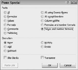
Figure 2.8. The "Formats" in the Values and Number Formats option pertains only to number formats such as currency, not to more broadly defined formats such as boldface and italics.
When you copy cell H12, you are copying its contents, and it contains a formula. When you then paste it into another cell, you are pasting that formula. If you try to paste it into, say, cell C3, you are pasting a formula that calls for the sum of values from one to six rows above the cell that contains the formula. But there aren't six rows above cell C3. Neither are there five rows above it, nor four, nor three.
Pasting a formula that refers to cells that don't exist always results in the #REF! error value, just as shown in Figure 2.7.
Here's the way to manage things, if you want to do something similar to what's shown in Figures 2.6 and 2.7 — assuming additionally that you want it to actually work:
In the exported QuickBooks report, select the cells that you want to move. In Figure 2.6, that's H12:J12.
You can choose Edit

Switch to the target worksheet, and select the cell where you want the paste operation to start. (This cell will contain whatever was in cell H12 in the QuickBooks export.)
Right-click the selected cell, or choose Edit, and then choose Paste Special. The Paste Special dialog box shown in Figure 2.8 appears.
In the Paste section, click the Values and Number Formats option, and then click OK.
Now, when the paste operation is complete, you have not formulas but values (and the number formats in use in the copied cells) in the target worksheet. With values, there are no missing cells for a formula to look for, and therefore no #REF! error values. What you have lost is access to the cells the formula was based on, but since you weren't copying those cells anyway you've lost nothing you need.
Tip
If you want to copy and paste several parts of the QuickBooks report to another I worksheet, it can be quicker to begin by converting all the formulas to values in one operation. Click Excel's Select All button, which is the rectangle to the left of the column A header and above the row 1 header, to select all the cells. Next do your copy, and paste-special back to their original location. Now all the formulas will have become values in the QuickBooks export, and you can copy and paste them directly to the target sheet.
In Figure 2.2 you'll notice that one of the options in the Export Report dialog box is to export the report to an existing Excel workbook. Using an existing Excel workbook can be an attractive option for several reasons:
You can store several different reports in the same Excel workbook.
You can store a QuickBooks report that is run after each of several different accounting periods in the same workbook.
If you have several different company files, you can store a balance sheet and income statement from each company in one summary Excel workbook.
You can run a QuickBooks report on each of several different product lines and have each copy of the report occupy a different worksheet in the same workbook.
And so on. To use an existing workbook, select the option labeled An Existing Excel Workbook (refer to Figure 2.2). When you select this option, the edit box and the Browse button become enabled.
Whatever your reason to store a QuickBooks report in an existing Excel workbook, there are a few minor points that will save you time in the long run. The two main issues to keep in mind are where the workbook is located and which worksheet to use.
If you want to use an existing workbook to store the exported report, you have to tell QuickBooks where to find the workbook. If you want, you can type its path and name directly into the edit box. But most of us find that it's a lot easier to click the Browse button and use the familiar Windows navigation windows to locate the file. When you get to the file, click the file's name and then click Open.
A couple of items to take care of before you start the export:
The target workbook must be closed.
You cannot export a QuickBooks report to an open, unsaved Excel workbook. The Export Report dialog box asks you to browse to the saved location of the target workbook, and an unsaved workbook by definition has no saved location.
If you try to export a QuickBooks report to an open, saved Excel workbook, QuickBooks will complain and refuse to comply. This situation comes about when you have saved the Excel workbook but have left the workbook open in the Excel application window.
If you encounter this problem, just switch to Excel and close the workbook, re-saving it if necessary. Then return to QuickBooks and proceed with the export. If a different user has the workbook open, you have two options: You can wait for the other user to finish and close the workbook (Excel has a notification option for this situation). Or you can use Windows to make a copy of the workbook and have QuickBooks export to the copy. Of course you'll first have to specify the name of the copy in the Export Report dialog box.
The workbook must be saved on a disk or network location visible to your logon.
If an existing file is closed, it must be saved somewhere. If the Excel file is sitting on a server, be sure that you're logged on with a user name that has permission to read and modify the file.
You have the option of exporting the report to a new or an existing worksheet in an existing workbook. To select a particular worksheet, select the Use an Existing Sheet in the Workbook option. When you do so, the list box becomes enabled so that you can choose among existing sheets.
And here too there are some considerations:
Overwriting existing data. If you choose to export a QuickBooks report to an existing worksheet, all data, formulas, and formats in that worksheet will be deleted by the export.
Deleting the contents of the existing worksheet might seem okay. All you're doing is replacing an older export with a newer one. And you may well be right to do so. QuickBooks' exporting tips even suggest this method.
As someone who has used Excel on a daily basis for about 20 years, as the author or co-author of more than 15 books on Excel, and as the recipient of several Microsoft Excel MVP awards, I offer you this advice: Don't.
The QuickBooks Export Tips notwithstanding (see the section "Ignoring the QuickBooks Export Tips" for more information), it's likely to get you into difficulties. And even if you have good reason to replace the contents of the existing worksheet, there are better ways to go about it. You're better off exporting to a new worksheet.
Exporting to a new worksheet. If you export a QuickBooks report to a new worksheet in an existing Excel workbook, you run no risk of overwriting existing data. Once QuickBooks has created the new worksheet, you'll want to find it, and it helps to keep in mind the following:
Every Excel workbook has an active sheet that you see when the workbook is open, and whose title bar is not dimmed if there is more than one sheet visible in different windows. Even a closed workbook has an active sheet. When you export to a new worksheet, QuickBooks puts that new worksheet immediately to the left of the active worksheet in the tab area. (This is consistent with Excel's behavior when you insert a worksheet via the Excel user interface.)
As Figure 2.2 shows, QuickBooks' Export Report dialog box has an Include a New Worksheet in the Workbook that Explains Excel Worksheet Linking checkbox. If you fill that checkbox and export the report to a new or an existing Excel workbook, QuickBooks adds another worksheet to the workbook named QuickBooks Export Tips. The Export Tips worksheet goes beyond the topic of worksheet linking and mentions some other issues.
The topic "Where did my worksheet go?" tells you where QuickBooks locates the worksheet in the workbook. Another tells you that you can suppress the QuickBooks Export Tips worksheet in the future by clearing the checkbox.
Then the tip sheet gets into cell linkages, and things start to fall apart. The basic idea is that you might want to export a QuickBooks report to an Excel worksheet. Then, you would put formulas into another Excel worksheet, formulas that link to cells in the exported worksheet, in places that make more sense to you — perhaps to structure a report that hits only certain highlights. (See the "Establishing Links" section for an example of how to create this type of link.)
The idea that the tip sheet is trying to get across is that once these links are set up, you can re-export data repeatedly to the source worksheet and see the values update accordingly in the target worksheet.
The Export Tip sheet refers to the worksheet you export to variously as QuickBooks summary report, your source worksheet, an existing worksheet, a QuickBooks data worksheet, the current report, and the exported data sheet which serves as data source. It may help to standardize the jargon; I refer to the sheet that you export the QuickBooks data to as the export sheet, and the sheet that you want to customize either for functional or esthetic purposes as the custom sheet.
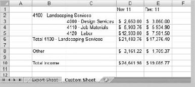
Figure 2.9 shows an export sheet with a Profit & Loss from QuickBooks.
Figure 2.10 shows the Profit & Loss in a custom sheet, as you want it to appear, for a board meeting perhaps, or just for your files, where you're not interested in maintaining subaccount information.
The way that the data in Figure 2.10 gets there is very different from the method outlined in the section "Moving Cells with Formulas." In the earlier section, you saw how to copy a formula and paste it into another cell as a value. The numbers in Figure 2.10 are also formulas, but they are formulas created by the user, not by QuickBooks. Figure 2.11 shows the data in Figure 2.9 (top) and Figure 2.10 (bottom), but instead of showing the results in the custom sheet as in Figure 2.10, it shows the formulas.

The most convenient, and probably the surest way to get those formulas into the custom sheet is to follow these steps (for just one cell — you'd have to adapt the steps slightly for other cells):
Select cell D3 in the custom sheet.
Type = (an equal sign).
To continue entering the formula, click in cell H5 in the export sheet. The formula should look like this:
='Export Sheet'!H5
Press Enter or click the green checkmark in the Formula Bar to establish the formula.
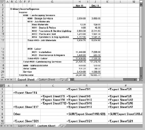
In words, the formula tells Excel to let cell D3 in the custom sheet equal whatever is contained in cell H5 in the export sheet. The Excel Export Tips sheet, as well as Excel itself, terms this formula a link.
In theory, this approach can be handy. It's a way to cherry-pick the values you want to see and skip the ones you don't. In this example, I'm cobbling together a report that shows income from parent accounts, and doesn't bother breaking those figures out by sub-subaccounts.
The preceding approach works best when the data source — in this case, the export sheet — does not vary from export to export. For example, suppose you export the income statement on November 11, and you would like the figure for Design Services in cell H5 to also appear in cell H5 when you export the income statement on December 11. The actual numeric figure may well be different a month later, but you would still hope to find it in the same cell as you did a month earlier.
In that case, the cells that the links in your custom sheet point to contain the same sort of information they did when you constructed them one or more months earlier: the values may differ, but if the cell contained a figure for Design Services in November's export, you expect it to contain a figure for Design Services in December's export. If you can depend on H5 in the export sheet to always contain Design Services income, regardless of when you export the report, then you can also depend on cell D3 in the custom sheet to display Design Services income.
But that's not what happens with QuickBooks reports. There are many ways that the P&L (or any QuickBooks report) can vary from month to month, simply as a function of normal financial events. The Export Tips sheet itself warns you of some of them, for example:
You have added, deleted, made active or deactivated even one item. This adds a row that wasn't there before in an item-driven report, or removes a row that was there before. Your formulas point to the same cells they did before, but the information in those cells is different: not just a different value, that's to be expected, but a different source for that value.
An account has activity during one period but not during another. Account-driven reports — reports that show different accounts on different lines — might rearrange themselves without letting you know. During November, for example, the income account named Books About Software might carry a $10 total. During December, when nobody buys books about software, that account might have no activity and disappear from the report. Then every subsequent line would get pulled up by one, but your links would still point at their original sources in the export sheet.
The QuickBooks' Export Tips worksheet recommends that before exporting you modify the report to show all rows. It does not tell you what to do about the fact that this modification snaps back to active rows when you're through. Sure, memorize the report, but are you certain you'll remember to use the memorized version next month? Furthermore, following that recommendation does not protect you against the consequences of adding a new item between exports.
Here's how to build more sophisticated links in Excel: links that will survive even if your report's rows unexpectedly appear or disappear between the dates that you run your report.
This approach is based on the fact that many QuickBooks reports can be depended on to always have certain important labels, and that they are always in the same columns. For example, regardless of the company file or when you create the report, the Balance Sheet Standard report has these labels in an export to an Excel worksheet:
Total Current Assets in column B
XXXX Inventory Asset in column D (where XXXX is an account number, if used)
Total Current Liabilities in column C
Suppose you want to create a custom report that shows your company's Current Ratio and its Quick Ratio. You want to glance at these ratios each month. Your approach is to export a Balance Sheet Standard report to an existing workbook at the end of each month. The report will always be exported to the same worksheet in that workbook.
Your custom sheet will contain links to the export sheet, and your immediate goal is to structure those links so that they work even if rows in the export sheet come and go from month to month. These links take just a little more time to create than do the simple point-and-shoot links explained in the prior section. But because you will use them over and over again, without having to worry about whether you structured the export report properly, the benefits are well worth the upfront time.
Figure 2.12 shows an example of the export sheet and the custom sheet.
Start by copying the labels of the values you're interested in seeing from the export sheet to the custom sheet. In this case, you want the building blocks of the current ratio and the quick ratio: total current assets, inventory assets, and total current liabilities. Copy these labels from cells B18, D15, and C44, respectively, in the export sheet and paste them into cells A2, A4, and A6 in the custom sheet. (The result is shown in Figure 2.12, column A in the custom sheet.)
Next, you want to build a formula in the custom sheet that finds the Total Current Assets label in the export sheet and displays the dollar figure associated with the label. To do so, start with Excel's MATCH function. In the custom report sheet, you would start by entering this formula, which uses MATCH, in cell B2:
=MATCH(A2,Export!B:B,0)
The formula returns the value 18, meaning that the value in A2, Total Current Assets, is matched by the value in the 18th row column B in the sheet named Export. The general syntax of the MATCH function is:
=MATCH(value to match, search location, match type)
where, in this case:
Total Current Assets is the value to match,
Column B in the sheet named Export is where to look for a match, and
0 is the match type, meaning that values in the search location are not necessarily in ascending numeric or alphabetical order.
The point is to locate the Total Current Assets value in the export sheet, regardless of how many rows precede it, therefore, regardless of which accounts appear in the report. Once you have located that label, it's easy to find the dollar amount associated with it. Meet Excel's OFFSET function:
=OFFSET(Export!$A$1,17,6)

Figure 2.12. If your company has cash, A/R amounts, undeposited funds, or inventory, it has current assets.
This formula, making use of OFFSET, returns the value 151178.40. That is the value in the cell offset by 17 rows and 6 columns from cell A1 in the sheet named Export. Not coincidentally, it's the amount of the total current assets shown in the balance sheet report.
Tip
Notice the dollar signs in the reference to cell A1 in the OFFSET formula. The $'s make it what Excel terms an absolute reference. If you copy the formula and paste it to a different cell, it will still refer to cell A1. In contrast, a relative reference to cell A1, without the dollar signs, would change, depending on how many rows down or columns across you pasted it into. By using the absolute reference, you can more easily replicate the formula in other cells, to pick up the inventory asset and the total current liabilities.
How do you know to use 17 rows and 6 columns in the OFFSET function? Well, in the standard balance sheet report, the dollar figures are always found in column G of the exported worksheet. Column G is the seventh column — it is offset six columns from cell A1.
The value Total Current Assets is found in the 18th row of column B, located there by the MATCH function described earlier. Therefore, it's offset by 17 rows from cell A1.
If you take the six-column offset as a constant, and by using MATCH allow for a variable number of rows to appear before the Total Current Assets value, you can get the associated dollar value directly by nesting MATCH within OFFSET:
=OFFSET(Export!$A$1,MATCH(A2,Export!B:B,0)-1,6)
to return, using just one formula, the value for the total current assets in the export sheet from QuickBooks
Tip
When you work with more complex formulas like this one, peek inside the formula to see what's going on. One way is to select the cell that contains the formula, click the Formula tab, and click Evaluate Formula in the Formula Auditing group (prior to Excel 2007, choose Tools
Now two more simple steps will give you the value for the inventory asset and the total current liabilities:
Copy the formula from its location in cell B2 in the custom sheet (shown in Figure 2.12) and paste it into cells B4 and B6, immediately to the right of the labels in column A that you're looking for in the export sheet.
For the inventory value, change B:B in the formula to D:D, so Excel will know which column to look in for the inventory asset label. For the current liabilities, change B:B to C:C, for the same reason.
The reference to cell A2, in the formula that picks up the total current assets, is a relative reference. Therefore, when you copy and paste it into cells B4 and B6, it automatically adjusts to a reference to A4 and A6. You will wind up with these formulas in cells B4 and B6:
=OFFSET(Export!$A$1,MATCH(A4,Export!D:D,0)-1,6)
=OFFSET(Export!$A$1,MATCH(A6,Export!C:C,0)-1,6)
To get the current ratio, enter this formula in cell B9 (or whatever other cell you prefer):
=B2/B6
and for the quick ratio (which removes inventory from the current assets to better estimate the assets that are already cash or that can be converted to cash quickly):
=(B2-B4)/B6
If this is your first time through this sort of formula development, it might seem complicated and unduly exacting. By the time you've done it three or four times it starts to seem old hat. Bear these points in mind:
You need do it only once, in your custom sheet.
Regardless of what changes push the row containing the current assets (or the inventory asset or the current liabilities) up or down in your export sheet, the
MATCHandOFFSETfunctions cause your formulas to return the correct values for the ratios you want.
And you don't have to worry about all those warnings in the QuickBooks Export Tips worksheet.
In Figure 2.2 you'll notice that your first available option is to export to a comma-separated values (CSV) file, which has the filename extension .csv. A CSV file can be used as a data source for most applications that work with user-supplied data: for example, a spreadsheet program such as Excel, a presentation program such as Adobe Acrobat, a database such as Oracle, or a statistical analysis package such as R. (QuickBooks can read data similar to CSV files too, but imposes extra requirements and refers to them as IIF files.)
A QuickBooks report exported to a CSV file has a particular structure, and it is much like an Excel worksheet list, or a data sheet in a database. Each row contains a different record, and each column contains a different field. If you are exporting a P&L or a balance sheet report, a field on the left corresponds to, say, a parent account, subaccount names appear in the next column, and sub-subaccounts appear in the subsequent columns. The final column or columns is for the numbers that apply to the accounts.
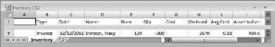
Figure 2.13 shows a CSV file as it appears in a simple application like Notepad:
The ninth row in the file is:
,"Invoice","12/12/2011","Stinson, Tracy", "129",-200,"",2670,0.18,480.6
There are nine fields in each row of this CSV file. Each pair of adjacent fields is separated by a comma. Text fields, such as customer name, are surrounded by quote marks (and may include a comma that doesn't separate two fields). Empty fields, where there is no value given for a particular record, are indicated by consecutive commas (,,) or in text fields by two quotation marks within commas (,"",). The ninth row shown earlier begins with an empty field; there's nothing to the left of the first comma.
Both Microsoft Excel and Microsoft Access recognize these patterns. Figure 2.14 shows how this row appears in an Excel worksheet.
QuickBooks export files that use the CSV structure are not as fancy as their Excel worksheet counterparts. For example:
The currency fields have no currency formats. If you open a CSV file in Excel, you see no dollar signs, thousands separators, or red fonts to indicate negative values.
Subtotals and totals are pure numeric values. In a direct export to an Excel worksheet, subtotals and totals are formulas using (normally) the
SUMfunction. (The absence of formulas is not necessarily a drawback. Even experienced Excel users sometimes insert an extraneous value where it will be used, erroneously, by an existing SUM function.)Particularly in reports that display information for subaccounts, the indenting you normally see might be absent. Figure 2.15 shows the same balance sheet, once as exported via a CSV file named
Balance Sheet.csvand opened in Excel, and as exported directly to an Excel worksheet. Note that the report exported directly to Excel uses indentation, and simulates section breaks by varying row heights (for example, rows 9 and 12 in Sheet1 in Figure 2.15).

Excel can distinguish numeric values from text, but you have to tell it if a field contains a currency value.
Generally, it makes more sense to export a report to an Excel worksheet than to a CSV file. If the export is to take advantage of Excel's broad scope of mathematical, financial, and statistical functions, there's usually little reason to take the extra step of exporting to a CSV file and then opening that file using Excel.
But if you want to put a QuickBooks report into an application such as a database, a CSV file makes good sense — and you don't even need a table in the database whose field structure matches the fields that you're going to export.
Why would you bother to import data from QuickBooks into a true database at all? There are several good reasons to import QuickBooks data into Excel. Excel has superior charting capabilities, analysis tools, and financial functions, and Excel can calculate key financial ratios. But a database, such as Access, SQL Server, or Oracle, has little of this sort of capability.

Figure 2.15. Notice that the indents indicating parent-subaccount relationships are missing from the CSV file.
In fact, you don't get much of a return by moving most QuickBooks reports into a true database. The standard reports are either almost all subtotals and totals (the summary reports) or individual records interspersed with subtotals and totals (the detail reports). Neither of these is much use in a database, which works best when all the records occupy the same level of detail.
One type of report, though, that you can move into a database to good effect is a custom transaction report. This report has great design flexibility. You can have subtotals if you want, using just about any field in your company file: account, item, customer, and so on. Or, if you want to handle data summaries in a different way, you can suppress subtotals, calling for totals only, and export the result to a CSV file for use in a database. Exported in this fashion, the records imported into the database are individual transactions.
Still, what's the point? Well, suppose that you want to analyze your business results by something other than QuickBook's built-in methods: items, or customers, or accounts, or fiscal years, and so on. What if you market to four regions of the country and want to view your revenues by region? Or, what if you have several different kinds of business to transact — say, Design, Landscaping, and Maintenance — and you want to see which business is the most profitable over time?
That's why QuickBooks provides the option of assigning transactions to a class. You can enable classes for a company file by choosing Edit
The difficulty arises when you want to use the class to represent different ways of slicing up your results. Suppose that in addition to line of business or geographic region, you also want to categorize transactions according to a department, say, Catalog Sales and Direct Sales. You can create these two new classes to represent your departments by choosing Lists
Setting up the two new classes to represent departments isn't the problem. The problem is that you can assign only one class to a given transaction. If you sell 12 argyle sweaters via your catalog to a customer in Idaho, do you assign that transaction to the Catalog class or to the Northwest class? You can't assign it to both since a given transaction can belong to one class only.
The usual advice is to create subclasses. So Catalog and Direct could be subclasses of Northwest, subclasses of Northeast, and so on. The subclass approach can sometimes be a good solution, but not in this case. Beyond the simple esthetics of having to look at something such as Northwest:Catalog Sales, or Design:Direct Sales (you can't suppress a parent class the way you can suppress a parent account) there is the more important issue of properly representing reality. It would make sense if you were to define the sales territories of Washington, Oregon, and Idaho as sub-classes of a Northwest class: states are logically and, usually, structurally subordinate to regions in a company's organization.
But distribution channels, such as catalog sales and direct sales, are not normally subordinate to regions. Channels cross regions; they are not nested within them. The same is often true of sales channels and lines of business.
So, to develop a way to classify transactions using more than one type of class, you normally need to go beyond the fields that QuickBooks gives you. Furthermore, true databases are ideally suited to adding new fields to a data set. (Better even than Excel, which offers only rudimentary database management capabilities.)
QuickBooks custom fields don't help here, because they belong to customer records, vendor records, employee records, and item records. They do not belong to transactions, which is what you're looking for. Yes, you could create a sales rep named Catalog, but that doesn't put you in a position to analyze all direct sales versus all catalog sales. QuickBooks reports would contrast each sales rep versus the entire catalog.
Still, you're stuck with how to classify transactions along more than one dimension. One way involves using the reference number field in QuickBooks (titled Num in QuickBooks' reports that show individual transactions). Continuing the example, you might consider entering the letter "C" at the start of each transaction that is a Catalog sale and the letter "D" if it is a Direct sale. After the data has been exported to a CSV file and imported into a database, it's easy to add to the database a field named Sales Channel and populate it by an update query that uses the reference number. You'll see one way in the "Opening the CSV File in Access" section.
It's easy to open a CSV file in Excel. Suppose that you have exported a report to a CSV file on the Desktop. To open it in Excel, just take these steps:
Choose File
Use the Open window to browse to the Desktop.
Click the Files of Type list box at the bottom of the Open window and choose Text Files (*.prn, *.txt, *.csv). Only files with one of those three extensions will appear in the Open window.
Click the name of your exported CSV file and click Open.
With Access, you can create an entirely new table in a database just by importing the CSV file. Access will use any labels it finds in the file's first row as field names. Importing a CSV file is probably the most straightforward way to get data out of QuickBooks and into a database.
While Excel can open the CSV file directly using File
Click External Data on the Ribbon and click Text File.
In the Select the Source and Destination of the Data window, use the Browse button to navigate to the location of the CSV file. When you click Browse, the File Open window appears.
Browse to the location where you saved the CSV report export file. Text Files (*.txt; *. csv; *.tab; *.asc) is the default file type, so you'll see any CSV files that you've saved in that location.
Select the CSV file and click Open. You are returned to the Source and Destination of the Data window. At this point you choose whether to import the data into the database or link to the data source. This choice is conceptually similar to using values in a report exported to Excel, or using linked formulas (explained earlier in the "Doing it the expert way" section). Your choice has no effect on completing the wizard, so assume you accept the default Import, and click OK.
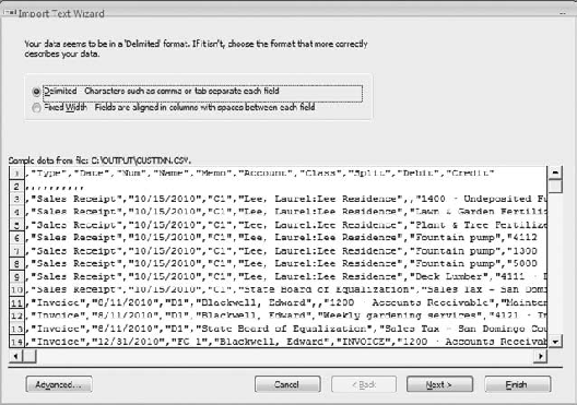
Click the Delimited or Fixed width option (see Figure 2.16). Because the fields in your file are delimited by commas, make sure the Delimited option is selected and click Next. (Files intended for a printer usually have fixed width columns and a .prn filename extension.)
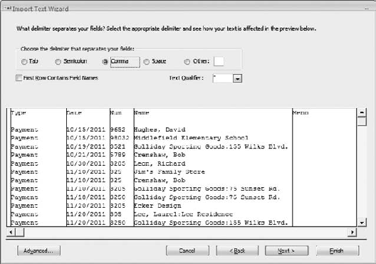
Select the Comma delimiter option (see Figure 2.17), choose the quotation mark from the list box as the text qualifier, and fill the First Row Contains Field Names checkbox. Most QuickBooks reports, including the Inventory Valuation reports, have columns with labels in the first row. However, the first column often has nothing in its first row, and the wizard will warn you of that situation. Access will replace a missing or unacceptable field name with something such as Field1. Dismiss the warning and click Next.
Next you can specify certain options for each field: the name the field will carry in the database, its numeric format, whether to skip the field, and whether to index it. It's a good idea to specify the Currency format for columns in a QuickBooks report that contains dollar values (see Figure 2.18). Do not index a field unless you're familiar with concepts such as primary keys and foreign keys. When you're finished, click Next.
Add a primary key to the table. A primary key is a value that uniquely identifies a record in a table in a database. All QuickBooks transactions and members of lists have primary keys, but you can't get at them through exported reports. The decision to use a primary key is much more complicated than is implied by this step (see Figure 2.19) but it will not slow things down much and could conceivably help. Choose Let Access Add a Primary Key and click Next.
In the wizard's final step, give the newly imported table a name and click Finish.
There's one more thing: Don't forget that the table is based on a QuickBooks report. That report has a total row, which you don't want in your database table. Scroll down to the bottom of the table to locate the total row, click to select it, and then press Delete to remove the row.
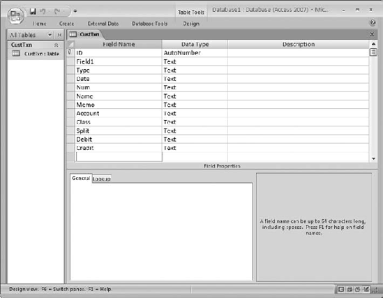
A portion of the imported table appears in Figure 2.20. Notice that the values in the Num field begin with either a C or a D: before the data was exported from QuickBooks, one or the other of those letters was added to indicate a Catalog or a Direct sale. The next task is to add a Sales Channel field to the database, and then classify the sales records according to their channel using the Num field. Here are the specific steps:
Click the Home tab on the Ribbon and choose Design View from the View list box. The window shown in Figure 2.21 appears.
Click the first empty cell in the Field Name column, and type a name for the new Sales Channel field.
Tip
In Access, names without embedded blanks are a little easier to deal with and you might consider a name such as SalesChannel or Sales_Channel.
On the same row, click in the cell in the Data Type column and choose Text in the list box.
Close the table by clicking the X in its upper-right corner. Respond Yes when Access asks you if you want to save changes to the table.

Figure 2.18. Click anywhere in a column to select it and specify its attributes, such as numeric format and whether to skip the field.

Figure 2.19. A primary key must have unique values, and QuickBooks reports provide no field that you can depend on to have a different value on each record.
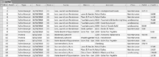
Figure 2.20. Access assigned the previously unnamed field the name FIELD1. You can change it later if you want.
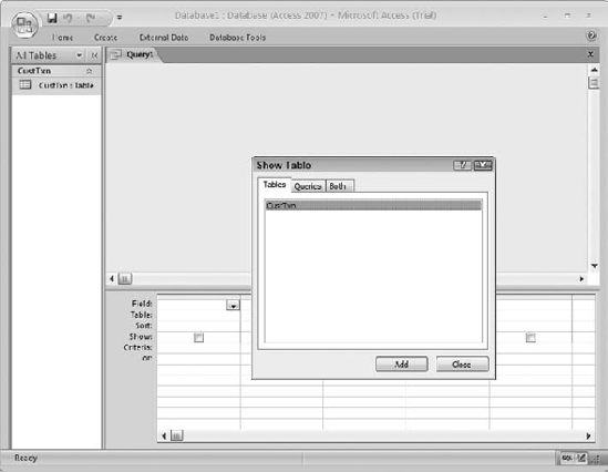
With the new field — which will contain the classes QuickBooks could not manage separately from the existing Class — defined, you can create an update query to populate the new field. Click the Create tab and click Query Design on the Ribbon (see Figure 2.22).
With just one table, it will be selected in the Show Table window. Click Add and then click Close.
Click Update in the Query Type group. The query design grid changes and will appear as shown in Figure 2.23.
Click the Num field from the data table and drag it to the cell in the design grid's first column, in its Field row.
Click in the first column's Criteria row and type
Left([Num],1)="C"
This expression, used as a criterion, tells Access to work only with records that have the letter "C" as their leftmost single character; that is, if the one character at the left end of the Num value is "C," include that record among those to process.
Click and drag the Sales Channel field name from the data table to the design grid's second column, in its Field row.
Click in the second column's Update To row and type this value, including the quote marks: "Catalog". The query window should now appear as shown in Figure 2.23.
Click Run in the Results group. The query runs, putting the value "Catalog" in the Sales Channel field for all records whose Num field begins with "C."
To get the "Direct" values into the Sales Channel field, change "C" to "D" in the design grid's Criteria row, and change "
Catalog" to "Direct" in the Update To row. Then click Run again.
To see the results of your query, double-click the table in the Navigation pane to open it in datasheet view. You will see the values in the Sales Channel field that correspond to the values you used in the update query: in this example, Catalog and Direct. See Figure 2.24 for an example.
But the datasheet view is too detailed to tell you much about how, if at all, Sales Channel and the Class you're using interact to bring about different levels of revenue or profit. The best way is by means of a pivot table.
Microsoft Access does offer pivot tables, but they are not as fully functioned or informative as are pivot tables in Excel. The next section shows you how to build a pivot table in Access, and one way to get the pivot table into Excel.
Once you have created a table in Access based on a CSV file from QuickBooks, most of the heavy lifting is finished and you're just a few mouse clicks away from a true data analysis. If you've followed the information and instructions in the prior section, you now have a table open in Access. To get a look at that table in a way that gives you some management information, follow these steps:
With a table open, click the Home tab if necessary and then choose PivotTable view from the View list box in the Views group. A window that shows the schematic for a pivot table appears as shown in Figure 2.25.

Figure 2.23. To see what the query looks like in Structured Query Language, click the View list box in the Results group and click SQL View.
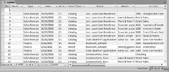
Figure 2.24. You should delete the first data row: it's just a blank row in the QuickBooks report that separates the column headers from the data.
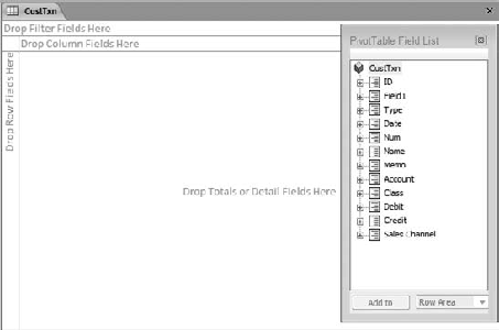
Figure 2.25. The Filter Fields area works much as does the Page Fields area in an Excel pivot table.
If you don't see the PivotTable Field List box shown in Figure 2.25, click the Field List button in the Show/Hide group on the Design tab. Drag the Class icon into the rectangle in the table schematic labeled Drop Row Fields Here.
Drag the Sales Channel icon into the rectangle labeled Drop Column Fields Here.
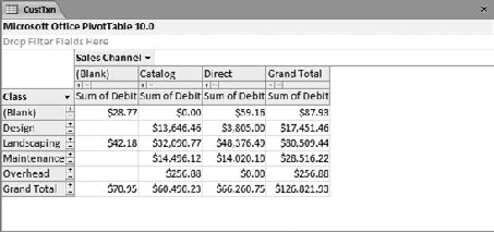
Drag the Debit icon into the main body of the schematic, labeled Drop Totals or Detail Fields Here.
At first you might see individual Debit values in the pivot table's data area, as shown in Figure 2.26. You can get sums of dollar values for each combination of Class and Sales Channel by clicking the Hide Details (the − [minus sign] icon) next to each value of either the Class field or the Sales Channel Field. When you do so, the pivot table appears as shown in Figure 2.27.

Tip
If your pivot table appears like the one in Figure 2.27 but no sums appear, make sure that you have defined the Debit field as Currency (begin by clicking View
This type of analysis is not feasible in QuickBooks. You sometimes need to export transaction data (or even list data) out of QuickBooks and into an application that might not be intended for bookkeeping, but that performs powerful numeric analysis.
Pivot tables in Access are useful, but they're even more useful in Excel. You can export the pivot table you created In Access to an Excel workbook; it will retain all the functionality it has in Access. Just click the Ribbon's Design tab, and then click Export to Excel in the Data group.