
7
Feature Extraction and Selection
In some cases, the dimension N of a measurement vector z, that is the number of sensors, can be very high. In image processing, when raw image data are used directly as the input for a classification, the dimension can easily attain values of 104 (a 100 × 100 image) or more. Many elements of z can be redundant or even irrelevant with respect to the classification process.
For two reasons, the dimension of the measurement vector cannot be taken arbitrarily large. The first reason is that the computational complexity becomes too large. A linear classification machine requires on the order of KN operations (K is the number of classes; see Chapter 4). A quadratic machine needs about KN2 operations. For a machine acting on binary measurements the memory requirement is on the order of K2N. This, together with the required throughput (number of classifications per second), the state of the art in computer technology and the available budget define an upper bound to N.
A second reason is that an increase of the dimension ultimately causes a decrease in performance. Figure 7.1 illustrates this. Here we have a measurement space with the dimension N varying between 1 and 13. There are two classes (K = 2) with equal prior probabilities. The (true) minimum error rate Emin is the one that would be obtained if all class densities of the problem were fully known. Clearly, the minimum error rate is a non-increasing function of the number of sensors. Once an element has been added with discriminatory information, the addition of another element cannot destroy this information. Therefore, with growing dimension, class information accumulates.

Figure 7.1 Error rates versus dimension of measurement space.
However, in practice the densities are seldom completely known. Often the classifiers have to be designed using a (finite) training set instead of using knowledge about the densities. In the example of Figure 7.1 the measurement data are binary. The number of states a vector can take is 2N. If there are no constraints on the conditional probabilities, then the number of parameters to estimate is on the order of 2N. The number of samples in the training set must be much larger than this. If not, overfitting occurs and the trained classifier will become too much adapted to the noise in the training data. Figure 7.1 shows that if the size of the training set is NS = 20, the optimal dimension of the measurement vector is about N = 4; that is where the error rate E is lowest. Increasing the sample size permits an increase of the dimension. With NS = 80 the optimal dimension is about N = 6.
One strategy to prevent overfitting, or at least to reduce its effect, has already been discussed in Chapter 6: incorporating more prior knowledge by restricting the structure of the classifier (for instance, by an appropriate choice of the discriminant function). In the current chapter, an alternative strategy will be discussed: the reduction of the dimension of the measurement vector. An additional advantage of this strategy is that it automatically reduces the computational complexity.
For the reduction of the measurement space, two different approaches exist. One is to discard certain elements of the vector and to select the ones that remain. This type of reduction is feature selection. It is discussed in Section 7.2. The other approach is feature extraction. Here the selection of elements takes place in a transformed measurement space. Section 7.3 addresses the problem of how to find suitable transforms. Both methods rely on the availability of optimization criteria. These are discussed in Section 7.1.
7.1 Criteria for Selection and Extraction
The first step in the design of optimal feature selectors and feature extractors is to define a quantitative criterion that expresses how well such a selector or extractor performs. The second step is to do the actual optimization, that is to use that criterion to find the selector/extractor that performs best. Such an optimization can be performed either analytically or numerically.
Within a Bayesian framework ‘best’ means the one with minimal risk. Often, the cost of misclassification is difficult to assess or is even fully unknown. Therefore, as an optimization criterion the risk is often replaced by the error rate E. Techniques to assess the error rate empirically by means of a validation set are discussed in Section 6.6. However, in this section we need to be able to manipulate the criterion mathematically. Unfortunately, the mathematical structure of the error rate is complex. The current section introduces some alternative, approximate criteria that are simple enough for a mathematical treatment.
In feature selection and feature extraction, these simple criteria are used as alternative performance measures. Preferably, such performance measures have the following properties:
- The measure increases as the average distance between the expectations vectors of different classes increases. This property is based on the assumption that the class information of a measurement vector is mainly in the differences between the class-dependent expectations.
- The measure decreases with increasing noise scattering. This property is based on the assumption that the noise on a measurement vector does not contain class information and that the class distinction is obfuscated by this noise.
- The measure is invariant to reversible linear transforms. Suppose that the measurement space is transformed to a feature space, that is y = Az with A an invertible matrix; then the measure expressed in the y space should be exactly the same as the one expressed in the z space. This property is based on the fact that both spaces carry the same class information.
- The measure is simple to manipulate mathematically. Preferably, the derivatives of the criteria are obtained easily as it is used as an optimization criterion.
From the various measures known in the literature (Devijver and Kittler, 1982), two will be discussed. One of them – the interclass/intraclass distance (Section 7.1.1) – applies to the multiclass case. It is useful if class information is mainly found in the differences between expectation vectors in the measurement space, while at the same time the scattering of the measurement vectors (due to noise) is class-independent. The second measure – the Chernoff distance (Section 7.1.2) – is particularly useful in the two-class case because it can then be used to express bounds on the error rate.
Section 7.1.3 concludes with an overview of some other performance measures.
7.1.1 Interclass/Intraclass Distance
The inter/intra distance measure is based on the Euclidean distance between pairs of samples in the training set. We assume that the class-dependent distributions are such that the expectation vectors of the different classes are discriminating. If fluctuations of the measurement vectors around these expectations are due to noise, then these fluctuations will not carry any class information. Therefore, our goal is to arrive at a measure that is a monotonically increasing function of the distance between expectation vectors and a monotonically decreasing function of the scattering around the expectations.
As in Chapter 6, TS is a (labelled) training set with NS samples. The classes ωk are represented by subsets Tk ⊂ TS, each class having Nk samples (∑Nk = NS). Measurement vectors in TS – without reference to their class – are denoted by zn. Measurement vectors in Tk (i.e. vectors coming from class ωk) are denoted by zk,n.
The development starts with the following definition of the average squared distance of pairs of samples in the training set:

The summand (zn–zm)T (zn–zm) is the squared Euclidean distance between a pair of samples. The sum involves all pairs of samples in the training set. The divisor N2S accounts for the number of terms.
The distance ![]() is useless as a performance measure because none of the desired properties mentioned above are met. Moreover,
is useless as a performance measure because none of the desired properties mentioned above are met. Moreover, ![]() is defined without any reference to the labels of the samples. Thus, it does not give any clue about how well the classes in the training set can be discriminated. To correct this,
is defined without any reference to the labels of the samples. Thus, it does not give any clue about how well the classes in the training set can be discriminated. To correct this, ![]() must be divided into a part describing the average distance between expectation vectors and a part describing distances due to noise scattering. For that purpose, estimations of the conditional expectations (
must be divided into a part describing the average distance between expectation vectors and a part describing distances due to noise scattering. For that purpose, estimations of the conditional expectations (![]() k = E[z|ωk]) of the measurement vectors are used, along with an estimate of the unconditional expectation (
k = E[z|ωk]) of the measurement vectors are used, along with an estimate of the unconditional expectation (![]() = E[z]). The sample mean of class ωk is
= E[z]). The sample mean of class ωk is

The sample mean of the entire training set is

With these definitions, it can be shown (see Exercise 1) that the average squared distance is

The first term represents the average squared distance due to the scattering of samples around their class-dependent expectation. The second term corresponds to the average squared distance between class-dependent expectations and the unconditional expectation.
An alternative way to represent these distances is by means of scatter matrices. A scatter matrix gives some information about the dispersion of a population of samples around their mean. For instance, the matrix that describes the scattering of vectors from class ωk is

Comparison with Equation (6.14) shows that Sk is close to an unbiased estimate of the class-dependent covariance matrix. In fact, Sk is the maximum likelihood estimate of Ck. Thus Sk does not only supply information about the average distance of the scattering, it also supplies information about the eccentricity and orientation of this scattering. This is analogous to the properties of a covariance matrix.
Averaged over all classes the scatter matrix describing the noise is

This matrix is the within-scatter matrix as it describes the average scattering within classes. Complementary to this is the between-scatter matrix Sb that describes the scattering of the class-dependent sample means around the overall average:

Figure 7.2 illustrates the concepts of within-scatter matrices and between-scatter matrices. The figure shows a scatter diagram of a training set consisting of four classes. A scatter matrix S corresponds to an ellipse, zS–1zT = 1, which can be thought of as a contour roughly surrounding the associated population of samples. Of course, strictly speaking the correspondence holds true only if the underlying probability density is Gaussian-like. However, even if the densities are not Gaussian, the ellipses give an impression of how the population is scattered. In the scatter diagram in Figure 7.2 the within-scatter Sw is represented by four similar ellipses positioned at the four conditional sample means. The between-scatter Sb is depicted by an ellipse centred at the mixture sample mean.

Figure 7.2 The interclass/intraclass distance.
With the definitions in Equations (7.5), (7.6) and (7.7) the average squared distance in (7.4) is proportional to the trace of the matrix Sw + Sb (see Equation (B.22)):
Indeed, this expression shows that the average distance is composed of a contribution due to differences in expectation and a contribution due to noise. The term JINTRA = trace(Sw) is called the intraclass distance. The term JINTER = trace(Sb) is the interclass distance. Equation (7.8) also shows that the average distance is not appropriate as a performance measure, since a large value of ![]() does not imply that the classes are well separated, and vice versa.
does not imply that the classes are well separated, and vice versa.
A performance measure more suited to express the separability of classes is the ratio between interclass and intraclass distance:
This measure possesses some of the desired properties of a performance measure. In Figure 7.2, the numerator, trace(Sb), measures the area of the ellipse associated with Sb. As such, it measures the fluctuations of the conditional expectations around the overall expectation, that is the fluctuations of the ‘signal’. The denominator, trace(Sw), measures the area of the ellipse associated with Sw. Therefore, it measures the fluctuations due to noise. Thus trace(Sb)/trace(Sw) can be regarded as a ‘signal-to-noise ratio’.
Unfortunately, the measure of Equation (7.9) oversees the fact that the ellipse associated with the noise can be quite large, but without having a large intersection with the ellipse associated with the signal. A large Sw can be quite harmless for the separability of the training set. One way to correct this defect is to transform the measurement space such that the within-scattering becomes white, that is Sw = I. For that purpose, we apply a linear operation to all measurement vectors yielding feature vectors yn = Azn. In the transformed space the within- and between-scatter matrices become ASwAT and ASbAT, respectively. The matrix A is chosen such that ASwAT = I.
The matrix A can be found by factorization: Sw = V![]() VT, where
VT, where ![]() is a diagonal matrix containing the eigenvalues of Sw and V is a unitary matrix containing the corresponding eigenvectors (see Appendix B.5). With this factorization it follows that A =
is a diagonal matrix containing the eigenvalues of Sw and V is a unitary matrix containing the corresponding eigenvectors (see Appendix B.5). With this factorization it follows that A = ![]() –1/2VT. An illustration of the process is depicted in Figure 7.2. The operation VT performs a rotation that aligns the axes of Sw. It decorrelates the noise. The operation
–1/2VT. An illustration of the process is depicted in Figure 7.2. The operation VT performs a rotation that aligns the axes of Sw. It decorrelates the noise. The operation ![]() –1/2 scales the axes. The normalized within-scatter matrix corresponds with a circle with unit radius. In this transformed space, the area of the ellipse associated with the between-scatter is a usable performance measure:
–1/2 scales the axes. The normalized within-scatter matrix corresponds with a circle with unit radius. In this transformed space, the area of the ellipse associated with the between-scatter is a usable performance measure:

This performance measure is called the inter/intra distance. It meets all of our requirements stated above.
Example 7.1 Interclass and intraclass distance
Numerical calculations of the example in Figure 7.2 show that before normalization JINTRA = trace(Sw) = 0.016 and JINTER = trace(Sb) = 0.54. Hence, the ratio between these two is JINTER/JINTRA = 33.8. After normalization, JINTRA = N = 2, JINTER = JINTER/INTRA = 59.1 and JINTER/JINTRA = trace(Sb)/trace(Sw) = 29.6. In this example, before normalization, the JINTER/JINTRA measure is too optimistic. The normalization accounts for this phenomenon.
7.1.2 Chernoff–Bhattacharyya Distance
The interclass and intraclass distances are based on the Euclidean metric defined in the measurement space. Another possibility is to use a metric based on probability densities. Examples in this category are the Chernoff distance (Chernoff, 1952) and the Bhattacharyya distance (Bhattacharyya, 1943). These distances are especially useful in the two-class case.
The merit of the Bhattacharyya and Chernoff distance is that an inequality exists where the distances bound the minimum error rate Emin. The inequality is based on the following relationship:
The inequality holds true for any positive quantities a and b. We will use it in the expression of the minimum error rate. Substitution of Equation (3.15) in (3.16) yields

Together with Equation (7.11) we have the following inequality:
The inequality is called the Bhattacharyya upper bound. A more compact notation of it is achieved with the so-called Bhattacharyya distance. This performance measure is defined as
The Bhattacharyya upper bound then simplifies to
The bound can be made tighter if inequality (7.11) is replaced with the more general inequality min {a, b} ≤ asb1-s. This last inequality holds true for any s, a and b in the interval [0, 1]. The inequality leads to the Chernoff distance, defined as
Application of the Chernoff distance in derivation similar to Equation (7.12) yields
The so-called Chernoff bound encompasses the Bhattacharyya upper bound. In fact, for s = 0.5 the Chernoff distance and the Bhattacharyya distance are equal: JBHAT = JC(0.5).
There also exists a lower bound based on the Bhattacharyya distance. This bound is expressed as
A further simplification occurs when we specify the conditional probability densities. An important application of the Chernoff and Bhattacharyya distance is the Gaussian case. Suppose that these densities have class-dependent expectation vectors µk and covariance matrices Ck, respectively. Then it can be shown that the Chernoff distance transforms into

It can be seen that if the covariance matrices are independent of the classes, for example C1 = C2, the second term vanishes and the Chernoff and the Bhattacharyya distances become proportional to the Mahalanobis distance SNR given in Equation (3.46): JBHAT = SNR/8. Figure 7.3(a) shows the corresponding Chernoff and Bhattacharyya upper bounds. In this particular case, the relation between SNR and the minimum error rate is easily obtained using expression (3.47). Figure 7.3(a) also shows the Bhattacharyya lower bound.

Figure 7.3 Error bounds and the true minimum error for the Gaussian case (C1 = C2). (a) The minimum error rate with some bounds given by the Chernoff distance. In this example the bound with s = 0.5 (Bhattacharyya upper bound) is the most tight. The figure also shows the Bhattacharyya lower bound. (b) The Chernoff bound with dependence on s.
The dependency of the Chernoff bound on s is depicted in Figure 7.3(b). If C1 = C2, the Chernoff distance is symmetric in s and the minimum bound is located at s = 0.5 (i.e. the Bhattacharyya upper bound). If the covariance matrices are not equal, the Chernoff distance is not symmetric and the minimum bound is not guaranteed to be located midway. A numerical optimization procedure can be applied to find the tightest bound.
If in the Gaussian case the expectation vectors are equal (![]() 1 =
1 = ![]() 2), the first term of Equation (7.19) vanishes and all class information is represented by the second term. This term corresponds to class information carried by differences in covariance matrices.
2), the first term of Equation (7.19) vanishes and all class information is represented by the second term. This term corresponds to class information carried by differences in covariance matrices.
7.1.3 Other Criteria
The criteria discussed above are certainly not the only ones used in feature selection and extraction. In fact, large families of performance measures exist; see Devijver and Kittler (1982) for an extensive overview. One family is the so-called probabilistic distance measures. These measures are based on the observation that large differences between the conditional densities p(z|ωk) result in small error rates. Let us assume a two-class problem with conditional densities p(z|ω1) and p(z|ω2). Then a probabilistic distance takes the following form:
The function g(·,·) must be such that J is zero when p(z|ω1) = p(z|ω2), ∀z, and non-negative otherwise. In addition, we require that J attains its maximum whenever the two densities are completely non-overlapping. Obviously, the Bhattacharyya distance (7.14) and the Chernoff distance (7.16) are examples of performance measures based on a probabilistic distance. Other examples are the Matusita measure and the divergence measures:

These measures are useful for two-class problems. For more classes, a measure is obtained by taking the average of pairs. That is,

where Jk,l is the measure found between the classes ωk and ωl.
Another family is the one using the probabilistic dependence of the measurement vector z on the class ωk. Suppose that the conditional density of z is not affected by ωk, that is p(z|ωk.) = p(z),∀z; then an observation of z does not increase our knowledge of ωk. Therefore, the ability of z to discriminate class ωk from the rest can be expressed in a measure of the probabilistic dependence:
where the function g(·,·) must have similar properties to those in Equation (7.20). In order to incorporate all classes, a weighted sum of Equation (7.24) is formed to get the final performance measure. As an example, the Chernoff measure now becomes

Other dependence measures can be derived from the probabilistic distance measures in a likewise manner.
A third family is founded on information theory and involves the posterior probabilities P(ωk|z). An example is Shannon's entropy measure. For a given z, the information of the true class associated with z is quantified by Shannon by entropy:

Its expectation
is a performance measure suitable for feature selection and extraction.
7.2 Feature Selection
This section introduces the problem of selecting a subset from the N-dimensional measurement vector such that this subset is most suitable for classification. Such a subset is called a feature set and its elements are features. The problem is formalized as follows. Let F(N) = {zn|n = 0 ··· N 1} be the set with elements from the measurement vector z. Furthermore, let Fj (D) = {yd|d = 0 ··· D – 1} be a subset of F(N) consisting of D < N elements taken from z. For each element yd there exists an element zn such that yd = zn. The number of distinguishable subsets for a given D is
This quantity expresses the number of different combinations that can be made from N elements, each combination containing D elements and with no two combinations containing exactly the same D elements. We will adopt an enumeration of the index j according to: j = 1 ··· q (D).
In Section 7.1 the concept of a performance measure has been introduced. These performance measures evaluate the appropriateness of a measurement vector for the classification task. Let J(Fj (D)) be a performance measure related to the subset Fj(D). The particular choice of J(.) depends on the problem at hand. For instance, in a multiclass problem, the interclass/intraclass distance JINTER/INTRA(.) could be useful (see Equation (7.10)).
The goal of feature selection is to find a subset ![]() with dimension D such that this subset outperforms all other subsets with dimension D:
with dimension D such that this subset outperforms all other subsets with dimension D:
An exhaustive search for this particular subset would solve the problem of feature selection. However, there is one practical problem. How to accomplish the search process? An exhaustive search requires q(D) evaluations of J(Fj(D)). Even in a simple classification problem, this number is enormous. For instance, let us assume that N = 20 and D = 10. This gives about 2 × 10⁵ different subsets. A doubling of the dimension to N = 40 requires about 109 evaluations of the criterion. Needless to say that even in problems with moderate complexity, an exhaustive search is out of the question.
Obviously, a more efficient search strategy is needed. For this, many options exist, but most of them are suboptimal (in the sense that they cannot guarantee that the subset with the best performance will be found). In the remaining part of this section, we will first consider a search strategy called ‘branch-and-bound’. This strategy is one of the few that guarantees optimality (under some assumptions). Next, we continue with some of the much faster, but suboptimal, strategies.
7.2.1 Branch-and-Bound
The search process is accomplished systematically by means of a tree structure (see Figure 7.4). The tree consists of an N – D + 1 level. Each level is enumerated by a variable n with n varying from D up to N. A level consists of a number of nodes. A node i at level n corresponds to a subset Fi(n). At the highest level, n = N, there is only one node corresponding to the full set F(N). At the lowest level, n = D, there are q(D) nodes corresponding to the q(D) subsets among which the solution must be found. Levels in between have a number of nodes that is less than or equal to q(n). A node at level n is connected to one node at level n + 1 (except the node F(N) at level N). In addition, each node at level n is connected to one or more nodes at level n – 1 (except the nodes at level D). In the example of Figure 7.4, N = 6 and D = 2.

Figure 7.4 A top-down tree structure on behalf of feature selection.
A prerequisite of the branch-and-bound strategy is that the performance measure is a monotonically increasing function of the dimension D. The assumption behind it is that if we remove one element from a measurement vector, the performance can only become worse. In practice, this requirement is not always satisfied. If the training set is finite, problems in estimating large numbers of parameters may result in an actual performance increase when fewer measurements are used (see Figure 7.1).
The search process takes place from the highest level (n = N) by systematically traversing all levels until finally the lowest level (n = D) is reached. Suppose that one branch of the tree has been explored up to the lowest level and suppose that the best performance measure found so far at level n = D is ![]() . Consider a node Fi(l) (at a level n > D) which has not been explored as yet. Then, if J(Fi(n)) ×
. Consider a node Fi(l) (at a level n > D) which has not been explored as yet. Then, if J(Fi(n)) × ![]() , it is unnecessary to consider the nodes below Fi(n). The reason is that the performance measure for these nodes can only become less than J(Fi(n)) and thus less than
, it is unnecessary to consider the nodes below Fi(n). The reason is that the performance measure for these nodes can only become less than J(Fi(n)) and thus less than ![]() .
.
The following algorithm traverses the tree structure according to a depth first search with a backtrack mechanism. In this algorithm the best performance measure found so far at level n = D is stored in a variable ![]() Branches whose performance measure is bounded by
Branches whose performance measure is bounded by ![]() are skipped. Therefore, relative to exhaustive search the algorithm is much more computationally efficient. The variable S denotes a subset. Initially this subset is empty and
are skipped. Therefore, relative to exhaustive search the algorithm is much more computationally efficient. The variable S denotes a subset. Initially this subset is empty and ![]() is set to 0. As soon as a combination of D elements has been found that exceeds the current performance, this combination is stored in S and the corresponding measure in
is set to 0. As soon as a combination of D elements has been found that exceeds the current performance, this combination is stored in S and the corresponding measure in ![]() .
.
Algorithm 7.1 Branch-and-bound search
Input: a labelled training set on which a performance measure J() is defined.
- 1. Initiate:
 = 0 and S = φ.
 - 2. Explore-node (F1(N)).
Output: the maximum performance measure stored in ![]() with the associated subset of F1 (N) stored in S.
with the associated subset of F1 (N) stored in S.
Procedure: Explore-node (Fi(n)).
- 1. If (J(Fi(n)) ≤
 ) then return.
 - 2. If (n = D) then
- 2.1 If (J(Fi(n)) >
 ) then
 - 2.1.1.
 = J(Fi(n));
 - 2.1.2. S = Fi (n);
- 2.1.3. Return.
- 3. For all (Fj(n – 1) ⊂ Fi(n)) do Explore-node(Fj(n – 1)).
- 4. Return.
The algorithm is recursive. The procedure ‘Explore-node ()’ explores the node given in its argument list. If the node is not a leaf, all its children nodes are explored by calling the procedure recursively. The first call is with the full set F (N) as argument.
The algorithm listed above does not specify the exact structure of the tree. The structure follows from the specific implementation of the loop in step 3. This loop also controls the order in which branches are explored. Both aspects influence the computational efficiency of the algorithm. In Figure 7.4, the list of indices of elements that are deleted from a node to form the child nodes follows a specific pattern (see Exercise 2). The indices of these elements are shown in the figure. Note that this tree is not minimal because some twigs have their leaves at a level higher than D. Of course, pruning these useless twigs in advance is computationally more efficient.
7.2.2 Suboptimal Search
Although the branch-and-bound algorithm can save many calculations relative to an exhaustive search (especially for large values of q (D)), it may still require too much computational effort.
Another possible defect of branch-and-bound is the top-down search order. It starts with the full set of measurements and successively deletes elements. However, the assumption that the performance becomes worse as the number of features decreases holds true only in theory (see Figure 7.1). In practice, the finite training set may give rise to an overoptimistic view if the number of measurements is too large. Therefore, a bottom-up search order is preferable. The tree in Figure 7.5 is an example.
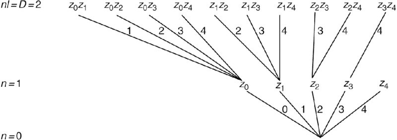
Figure 7.5 A bottom-up tree structure for feature selection.
Among the many suboptimal methods, we mention a few. A simple method is sequential forward selection (SFS). The method starts at the bottom (the root of the tree) with an empty set and proceeds its way to the top (a leaf) without backtracking. At each level of the tree, SFS adds one feature to the current feature set by selecting from the remaining available measurements the element that yields a maximal increase of the performance. A disadvantage of the SFS is that once a feature is included in the selected sets it cannot be removed, even if at a higher level in the tree, when more features are added, this feature would be less useful.
The SFS adds one feature at a time to the current set. An improvement is to add more than one, say l, features at a time. Suppose that at a given stage of the selection process we have a set Fj (n) consisting of n features. Then the next step is to expand this set with l features taken from the remaining N – n measurements. For that we have (N – n)! / ((N – n – l)! l!) combinations, which all must be checked to see which one is most profitable. This strategy is called the generalized sequential forward selection (GSFS (l)).
Both the SFS and the GSFS (l) lack a backtracking mechanism. Once a feature has been added, it cannot be undone. Therefore, a further improvement is to add l features at a time and after that to dispose of some of the features from the set obtained so far. Hence, starting with a set of Fj (n) features we select the combination of l remaining measurements that when added to Fj (n) yields the best performance. From this expanded set, say Fi (n + l), we select a subset of r features and remove it from Fi (n + l) to obtain a set, say Fk (n + l – r). The subset of r features is selected such that Fk (n + l – r) has the best performance. This strategy is called ‘Plus l – take away r selection’.
Example 7.2 Character classification for licence plate recognition
In traffic management, automated licence plate recognition is useful for a number of tasks, for example speed checking and automated toll collection. The functions in a system for licence plate recognition include image acquisition, vehicle detection, licence plate localization, etc. Once the licence plate has been localized in the image, it is partitioned such that each part of the image – a bitmap – holds exactly one character. The classes include all alphanumerical values. Therefore, the number of classes is 36. Figure 7.6(a) provides some examples of bitmaps obtained in this way.

Figure 7.6 Character classifications for licence plate recognition. (a) Character sets from licence plates, before and after normalization. (b) Selected features. The number of features is 18 and 50, respectively.
The size of the bitmaps ranges from 15 × 6 up to 30 × 15. In order to fix the number of pixels, and also to normalize the position, scale and contrasts of the character within the bitmap, all characters are normalized to 15 × 11.
Using the raw image data as measurements, the number of measurements per object is 15 × 11 = 165. A labelled training set consisting of about 70 000 samples, that is about 2000 samples/class, is available. Comparing the number of measurements against the number of samples/class we conclude that overfitting is likely to occur.
A feature selection procedure, based on the ‘plus l–take away r’ method (l = 3, r = 2) and the inter/intra distance (Section 7.1.1) gives feature sets as depicted in Figure 7.6(b). Using a validation set consisting of about 50 000 samples, it was established that 50 features gives the minimal error rate. A number of features above 50 introduces overfitting. The pattern of 18 selected features, as shown in Figure 7.6(b), is one of the intermediate results that were obtained to get the optimal set with 50 features. It indicates which part of a bitmap is most important to recognize the character.
7.2.3 Several New Methods of Feature Selection
Researchers have observed that feature selection is a combinatorial optimization issue. As a consequence, we can solve a feature selection problem with some approaches utilized for solving a combinatorial optimization issue. Many efforts have paid close attention to the optimization problem and some characteristic methods have been proposed in recent years. Here we will introduce several representative methods.
7.2.3.1 Simulated Annealing Algorithm
Simulated annealing is a probabilistic technique for approximating the global optimum of a given function. Specifically, it is metaheuristic to approximate global optimization in a large search space. For problems where finding the precise global optimum is less important than finding an acceptable global optimum in a fixed amount of time, simulated annealing may be preferable to alternatives such as brute-force search or gradient descent.
The name and inspiration come from annealing in metallurgy, a technique involving heating and controlled cooling of a material to increase the size of its crystals and reduce defects. Both are attributes of the material that depend on its thermodynamic free energy. Heating and cooling the material affects both the temperature and the thermodynamic free energy. While the same amount of cooling brings the same decrease in temperature, the rate of cooling dictates the magnitude of decrease in the thermodynamic free energy, with slower cooling producing a bigger decrease. Simulated annealing interprets slow cooling as a slow decrease in the probability of accepting worse solutions as it explores the solution space. Accepting worse solutions is a fundamental property of metaheuristics because it allows for a more extensive search for the optimal solution.
If the material status is defined with the energy of its crystals, the simulated annealing algorithm utilizes a simple mathematic model to describe the annealing process. Suppose that the energy is denoted with E(i) at the state i, then the following rules will be obeyed when the state changes from state i to state j at the temperature T:
- If E(j) ≤ E(i), then accept the case that the state is transferred.
- If E(j) > E(i), then the state transformation is accepted with a probability:
where K is a Boltzmann constant in physics and T is the temperature of the material.

The material will reach a thermal balance after a full transformation at a certain temperature. The material is in a status i with a probability meeting with a Boltzmann distribution:

where x denotes the random variable of current state of the material and S represents the state space set.
Obviously,

where |S| denotes the number of the state in the set S. This manifests that all states at higher temperatures have the same probability. When the temperature goes down,

where ![]() and Smin = {i: E(i) = Emin }.
and Smin = {i: E(i) = Emin }.
The above equation shows that the material will turn into the minimum energy state with a high probability when the temperature drops to very low.
Suppose that the problem needed to be solved is an optimization problem finding a minimum. Then applying the simulated annealing idea to the optimization problem, we will obtain a method called the simulated annealing optimization algorithm.
Considering such a combinatorial optimization issue, the optimization function is f: x → R+, where x ∈ S is a feasible solution, R+ = {y|y ∈ R, y > 0}, S denotes the domain of the function and N(x)⊆S represents a neighbourhood collection of x.
Firstly, given an initial temperature T0 and an initial solution x(0) of this optimization issue, the next solution x′ ∈ N(x(0)) is generated by x(0). Whether or not to accept x′ as a new solution x(1) will depend on the probability below:

In other words, if the function value of the generated solution x' is smaller than the one of the previous solution, we accept x(1) = x' as a new solution; Otherwise, we accept x' as a new solution with the probability ![]() .
.
More generally, for a temperature Ti and a solution x(k) of this optimization issue, we can generate a solution x'. Whether or not to accept x' as a new solution x(k + 1) will depend on the probability below:

After a lot of transformation at temperature Ti, we will obtain Ti + 1 < Ti by reducing the temperature Ti; then repeat the above process at temperature Ti + 1. Hence, the whole optimization process is an alternate process of repeatedly searching new resolution and slowly cooling.
Note that a new state x(k + 1) completely depends on the previous state x(k) for each temperature Ti, and it is independent of the previous states x(0), …, x(k − 1). Hence, this is a Markov process. Analysing the above simulated annealing steps with the Markov process theory, the results show that, if the probability of generating x′ from any a state x(k) follows a uniform distribution in N(x(k)) and the probability of accepting x′ meets with Equation (7.34), the distribution of the equilibrium state xi at temperature Ti can be described as

When the temperature T becomes 0, the distribution of xi will be

and
The above expressions show that, if the temperature drops very slowly and there are sufficient state transformations at each temperature, then the globally optimal solution will be found with the probability 1. In other words, the simulated annealing algorithm can find the globally optimal solution.
When we apply the simulated annealing algorithm to the feature selection, we first need to provide an initial temperature T0 > 0 and a group of initial features x(0). Then we need to provide a neighbourhood N(x) with respect to a certain group of features and the temperature dropping method. Here we will describe the simulated annealing algorithm for feature selection.
- Step 1: Let i = 0, k = 0, T0 denotes an initial temperature and x(0) represents a group of initial features.
- Step 2: Select a state x′ in the neighbourhood N(x(k)) of x(k), then compute the corresponding criteria J(x′) and accept x(k + 1) = x′ with the probability according to Equation (7.34).
- Step 3: If the equilibrium state cannot be arrived at, go to step 2.
- Step 4: If the current temperature Ti is low enough, stop computing and the current feature combination is the final result of the simulated annealing algorithm. Otherwise, continue.
- Step 5: Compute the new temperature Ti + 1 according to the temperature dropping method and then go to step 2.
Several issues should be noted.
- If the cooling rate is too slow, the performance of the solution obtained is good but the efficiency is low. As a result, there are not significant advantages relative to some simple searching algorithms. However, the final result obtained may not be the globally optimal solution if the cooling rate is too fast. The performance and efficiency should be taken into account when we utilize the algorithm.
- The stopping criterion should be determined for the state transformation at each temperature. In practice, the state transformation at a certain temperature can be stopped when the state does not change during a continuous m times transformation process. The final temperature can be set as a relatively small valueTe.
- The choice of an appropriate initial temperature is also important.
- The determination of the neighbourhood of a feasible solution should be carefully considered.
7.2.3.2 Tabu Search Algorithm
The tabu search algorithm is a metaheuristic search method employing local search methods used for mathematical optimization. Tabu search enhances the performance of local search by relaxing its basic rule. First, at each step worsening moves can be accepted if no improving move is available (such as when the search is stuck at a strict local mimimum). In addition, prohibitions (henceforth the term tabu) are introduced to discourage the search from coming back to previously visited solutions.
The implementation of tabu search uses memory structures that describe the visited solutions or user-provided sets of rules. If a potential solution has been previously visited within a certain short-term period or if it has violated a rule, it is marked as ‘tabu’ (forbidden) so that the algorithm does not consider that possibility repeatedly.
Tabu search uses a local or neighbourhood search procedure to iteratively move from one potential solution x to an improved solution x′ in the neighbourhood of x, until some stopping criterion has been satisfied (generally an attempt limit or a score threshold). Local search procedures often become stuck in poor-scoring areas or areas where scores plateau. In order to avoid these pitfalls and explore regions of the search space that would be left unexplored by other local search procedures, tabu search carefully explores the neighbourhood of each solution as the search progresses. The solutions admitted to the new neighbourhood, N(x), are determined through the use of memory structures. Using these memory structures, the search progresses by iteratively moving from the current solution x to an improved solution x′ in N(x).
These memory structures form what is known as the tabu list, a set of rules and banned solutions used to filter which solutions will be admitted to the neighbourhood N(x) to be explored by the search. In its simplest form, a tabu list is a short-term set of the solutions that have been visited in the recent past (less than n iterations ago, where n is the number of previous solutions to be stored – it is also called the tabu tenure). More commonly, a tabu list consists of solutions that have changed by the process of moving from one solution to another. It is convenient, for ease of description, to understand a ‘solution’ to be coded and represented by such attributes.
The basic framework of a tabu searching algorithm is described below:
- Step 1: Let the iterative step i = 0, the tabu table T = ∅, the initial solution is x and the optimal solution xg = x.
- Step 2: Select a number of solutions from the neighbourhood x to form the candidate solution set N(x).
- Step 3: If N(x) = ∅, then go to step 2. Otherwise, find the optimal solution x′ from N(x).
- Step 4: If x′ ∈ T and x′ does not meet the activation condition, then let N(x) = N(x) − {x′} and go to step 3. Otherwise, let x = x′.
- Step 5: If x is better than xg in performance, then xg = x.
- Step 6: If the length of the tabu table is equal to the specified length, then remove the solution search at the earliest.
- Step 7: Let T = T∪{x}.
- Step 8: If the algorithm meets with the stopping criterion, then stop the algorithm and output the final solution xg. Otherwise, let i = i + 1 and go to step 2.
When the above method is directly applied to feature selection, each solution x represents a kind of feature combination and its performance is measured with the separability criterion J.
Here we will discuss several important issues in the above algorithm.
- Step 5 can ensure that the final solution must be an optimal solution among all solutions searched.
- The tabu table records the solutions that possess better performance and are searched recently; the new candidate solution sets are based on the recent solutions in the tabu table. In order to obtain better solution with higher probability, we should make the candidate solution sets include the elements that have not been searched as far as possible. To this aim, one possible method is to generate the candidate solution set based on various solutions x as far as possible. Thus, a longer tabu table will extend the searching range, which will result in a better solution with higher probability. The length of the tabu table is an important issue. It is associated with the complexity of the optimization problem to be solved and it is also relevant to the method generating the candidate solution and the number of iterations. Of course, a longer table needs more storage memory and more computation time.
- The performance of the algorithm can also be influenced by the neighbourhood of a solution x and the choice of the candidate solutions. If the solution distribution can be taken into account when the neighbourhood and the candidate solution sets are generated, the neighbourhood and the candidate solution sets generated may have better performance. In addition, the number of candidate solutions is also an important parameter. Generally, a greater value means that more prohibition solutions will be accessed and the solution obtained may be better.
7.2.3.3 Genetic Algorithm
Genetic algorithms are a part of evolutionary computing, which is a rapidly growing area of artificial intelligence. Genetic algorithms are inspired by Darwin's theory about evolution. Simply said, the solution to a problem solved by genetic algorithms has evolved. Before we can explain more about a genetic algorithm, some terms about it will first be given.
- Gene encoding. The characters of biology are determined by the genetic code. In a genetic algorithm, each solution for a problem should be encoded as a genetic code. For example, suppose that an integer 1552 is a solution for a problem; then we can utilize its binary number as the corresponding genetic code and each bit represents a gene. Therefore, a genetic code represents a solution for a problem and each genetic code sometimes is called an individual.
- Population. A population is a set consisting of several individuals. Since each individual represents a solution for the problem, a population forms the solution set for the problem.
- Crossover. Select two individuals x1, x2 from the population and take the two individuals as a parent to implement the crossover of the genetic codes. As a result, two new individuals x′1, x′2 are generated. The simplest way to do this is to choose randomly some crossover point and everything before this point copy from a first parent and then everything after a crossover point copy from the second parent. There are other ways that can be used to make a crossover, for example we can choose more crossover points. Crossover can be rather complicated and very much depends on the genetic codes. A specific crossover made for a specific problem can improve the performance of the genetic algorithm.
- Mutation. After a crossover is performed, mutation takes place. This is to prevent placing all solutions in a population into a local optimum of a solved problem. Mutation randomly changes the new offspring. For binary encoding we can switch a few randomly chosen bits from 1 to 0 or from 0 to 1.
- Fitness. Each individual directly corresponds to a solution xi for the optimization problem and each solution xi directly corresponds to a function value fi. A greater fi (if the optimization problem requires a maximum) means that xi is a better solution, that is xi adapts to the surrounding environment better.
According to Darwin's theory of evolution, each individual in nature continually learns and fits its surrounding environment and those individuals generate new offspring by crossover, which is so-called genetic inheritance. After genetic inheritance, those offspring inherit excellent properties from their parents and continually learn and fit their surrounding environment. From an evolution perspective, new populations are stronger than their parents in advantage fitness for the surrounding environment.
The basic framework of genetic algorithm is described below:
- Step 1: Let evolution generation be t = 0.
- Step 2: Let P(t) represent the initial population and xg denote any individual.
- Step 3: Estimate the objective function value of each individual in P(t) and compare the optimal value x′ with xg. If the performance of x′ is better than xg, then set xg = x′.
- Step 4: If the stopping criterion is satisfied, then stop the algorithm and xg is regarded as the final result. Otherwise, go to step 5.
- Step 5: Select the individuals from P(t) and carry out the operation of crossover and mutation to obtain the new population P(t + 1). Let t = t + 1 and go to Step 3.
Here we will discuss several important issues in the above algorithm.
- Step 3 can ensure that the final solution must be an optimal solution among all solutions searched.
- The common stopping criteria are that the evolution generation is greater than a given threshold or there is not a more optimal solution after continuous evolution generations are given.
- The size of the population and the evolution generations are important parameters. Within certain limits, greater values of the two parameters can generate a better solution.
- In step 5, two individuals used for crossover can be selected with the following rules: If an individual possesses better performance, the probability selected should be greater.
When we apply a genetic algorithm to feature selection, we first need to encode each solution into a genetic code. To this aim, we can adopt the following simple encoding rules. For example, if the problem is to select d features from D original features, then we can utilize a binary string constituting D bits 0 or 1 to represent a feature combination, where the numerical value 1 denotes the corresponding feature to be selected and the numerical value 0 denotes the corresponding feature to be unselected. Obviously, there is an exclusive binary string that corresponds to any feature combination. In addition, the fitness function can be replaced with the separability criterion J.
7.2.4 Implementation Issues
PRTools offers a large range of feature selection methods. The evaluation criteria are implemented in the function feateval and are basically all inter/intra cluster criteria. Additionally, a κ-nearest neighbour classification error is defined as a criterion. This will give a reliable estimate of the classification complexity of the reduced dataset, but can be very computationally intensive. For larger datasets it is therefore recommended to use the simpler inter–intra-cluster measures.
PRTools also offers several search strategies, i.e. the branch-and-bound algorithm, plus-l-takeaway-r, forward selection and backward selection. Feature selection mappings can be found using the function featselm. The following listing is an example.
Listing 7.1 PRTools code for performing feature selection.
% Create a labeled dataset with 8 features, of which only 2
% are useful, and apply various feature selection methods
z = gendatd(200,8,3,3);
w=featselm(z, ’maha-s’, ’forward’,2);     % Forward selection
figure; clf; scatterd(z*w);
title([’forward: ’ num2str(+w{2})]);
w=featselm(z,’maha-s’, ’backward’,2);     % Backward selection
figure; clf; scatterd(z*w);
title([’backward: ’ num2str(+w{2})]);
w=featselm(z, ’maha-s’, ’b&b’,2);         % B&B selection
figure; clf; scatterd(z*w);
title([’b&b: ’ num2str(+w{2})]);
The function gendatd creates a dataset in which just the first two measurements are informative while all other measurements only contain noise (where the classes completely overlap). The listing shows three possible feature selection methods. All of them are able to retrieve the correct two features. The main difference is in the required computing time: finding two features out of eight is approached most efficiently by the forward selection method, while backward selection is the most inefficient.
7.3 Linear Feature Extraction
Another approach to reduce the dimension of the measurement vector is to use a transformed space instead of the original measurement space. Suppose that W(.) is a transformation that maps the measurement space ![]() on to a reduced space
on to a reduced space ![]() , D ≪ N. Application of the transformation to a measurement vector yields a feature vector
, D ≪ N. Application of the transformation to a measurement vector yields a feature vector
![]() :
:
Classification is based on the feature vector rather than on the measurement vector (see Figure 7.7).

Figure 7.7 Feature extraction.
The advantage of feature extraction above feature selection is that no information from any of the elements of the measurement vector needs to be wasted. Furthermore, in some situations feature extraction is easier than feature selection. A disadvantage of feature extraction is that it requires the determination of some suitable transformation W(.). If the transform chosen is too complex, the ability to generalize from a small dataset will be poor. On the other hand, if the transform chosen is too simple, it may constrain the decision boundaries to a form that is inappropriate to discriminate between classes. Another disadvantage is that all measurements will be used, even if some of them are useless. This might be unnecessarily expensive.
This section discusses the design of linear feature extractors. The transformation W(.) is restricted to the class of linear operations. Such operations can be written as a matrix–vector product:
where W is a D × N matrix. The reason for the restriction is threefold. First, a linear feature extraction is computationally efficient. Second, in many classification problems – though not all – linear features are appropriate. Third, a restriction to linear operations facilitates the mathematical handling of the problem.
An illustration of the computational efficiency of linear feature extraction is the Gaussian case. If covariance matrices are unequal, the number of calculations is on the order of KN2 (see Equation (3.20)). Classification based on linear features requires about DN + KD2 calculations. If D is very small compared with N, the extraction saves a large number of calculations.
The example of Gaussian densities is also well suited to illustrate the appropriateness of linear features. Clearly, if the covariance matrices are equal, then Equation (3.25) shows that linear features are optimal. On the other hand, if the expectation vectors are equal and the discriminatory information is in the differences between the covariance matrices, linear feature extraction may still be appropriate. This is shown in the example of Figure 3.10(b) where the covariance matrices are eccentric, differing only in their orientations. However, in the example shown in Figure 3.10(a) (concentric circles) linear features seem to be inappropriate. In practical situations, the covariance matrices will often differ in both shape and orientations. Linear feature extraction is likely to lead to a reduction of the dimension, but this reduction may be less than what is feasible with non-linear feature extraction.
Linear feature extraction may also improve the ability to generalize. If, in the Gaussian case with unequal covariance matrices, the number of samples in the training set is in the same order as that of the number of parameters, KN2, overfitting is likely to occur, but linear feature extraction – provided that D ≪ N – helps to improve the generalization ability.
We assume the availability of a training set and a suitable performance measure J(.). The design of a feature extraction method boils down to finding the matrix W that – for the given training set – optimizes the performance measure.
The performance measure of a feature vector y = Wz is denoted by J(y) or J(Wz). With this notation, the optimal feature extraction is
Under the condition that J(Wz) is continuously differentiable in W, the solution of Equation (7.37) must satisfy
Finding a solution of either Equation (7.40) or (7.41) gives us the optimal linear feature extraction. The search can be accomplished numerically using the training set. Alternatively, the search can also be done analytically assuming parameterized conditional densities. Substitution of estimated parameters (using the training set) gives the matrix W.
In the remaining part of this section, the last approach is worked out for two particular cases: feature extraction for two-class problems with Gaussian densities and feature extraction for multiclass problems based on the inter/intra distance measure. The former case will be based on the Bhattacharyya distance.
7.3.1 Feature Extraction Based on the Bhattacharyya Distance with Gaussian Distributions
In the two-class case with Gaussian conditional densities a suitable performance measure is the Bhattacharyya distance. In Equation (7.19) JBHAT implicitly gives the Bhattacharyya distance as a function of the parameters of the Gaussian densities of the measurement vector z. These parameters are the conditional expectations ![]() k and covariance matrices Ck. Substitution of y = Wz gives the expectation vectors and covariance matrices of the feature vector, that is W
k and covariance matrices Ck. Substitution of y = Wz gives the expectation vectors and covariance matrices of the feature vector, that is W![]() k and WCkWT, respectively. For the sake of brevity, let m be the difference between expectations of z:
k and WCkWT, respectively. For the sake of brevity, let m be the difference between expectations of z:
Then substitution of m, ![]() k and WCkWT in Equation (7.19) gives the Bhattacharyya distance of the feature vector:
k and WCkWT in Equation (7.19) gives the Bhattacharyya distance of the feature vector:

The first term corresponds to the discriminatory information of the expectation vectors; the second term to the discriminatory information of covariance matrices.
Equation (7.40) is in such a form that an analytic solution of (7.37) is not feasible. However, if one of the two terms in (7.40) is dominant, a solution close to the optimal one is attainable. We consider the two extreme situations first.
7.3.1.1 Equal Covariance Matrices
In the case where the conditional covariance matrices are equal, that is C = C1 = C2, we have already seen that classification based on the Mahalanobis distance (see Equation (3.41)) is optimal. In fact, this classification uses a 1 × N-dimensional feature extraction matrix given by
To prove that this equation also maximizes the Bhattacharyya distance is left as an exercise for the reader.
7.3.1.2 Equal Expectation Vectors
If the expectation vectors are equal, m = 0, the first term in Equation (7.43) vanishes and the second term simplifies to

The D × N matrix W that maximizes the Bhattacharyya distance can be derived as follows.
The first step is to apply a whitening operation (Appendix C.3.1) on z with respect to class ω1. This is accomplished by the linear operation ![]() –1/2VTz. The matrices V and
–1/2VTz. The matrices V and ![]() follow from factorization of the covariance matrix: C1 = V
follow from factorization of the covariance matrix: C1 = V![]() VT, where V is an orthogonal matrix consisting of the eigenvectors of C1 and
VT, where V is an orthogonal matrix consisting of the eigenvectors of C1 and ![]() is the diagonal matrix containing the corresponding eigenvalues. The process is illustrated in Figure 7.8. The figure shows a two-dimensional measurement space with samples from two classes. The covariance matrices of both classes are depicted as ellipses. Figure 7.8(b) shows the result of the operation
is the diagonal matrix containing the corresponding eigenvalues. The process is illustrated in Figure 7.8. The figure shows a two-dimensional measurement space with samples from two classes. The covariance matrices of both classes are depicted as ellipses. Figure 7.8(b) shows the result of the operation ![]() –1/2VT. The operation VT corresponds to a rotation of the coordinate system such that the ellipse of class ω1 lines up with the axes. The operation
–1/2VT. The operation VT corresponds to a rotation of the coordinate system such that the ellipse of class ω1 lines up with the axes. The operation ![]() –1/2 corresponds to a scaling of the axes such that the ellipse of ω1 degenerates into a circle. The figure also shows the resulting covariance matrix belonging to class ω2.
–1/2 corresponds to a scaling of the axes such that the ellipse of ω1 degenerates into a circle. The figure also shows the resulting covariance matrix belonging to class ω2.

Figure 7.8 Linear feature extractions with equal expectation vectors. (a) Covariance matrices with decision function. (b) Whitening of ω1 samples. (c) Decorrelation of ω2 samples. (d) Decision function based on one linear feature.
The result of the operation ![]() –1/2VT on z is that the covariance matrix associated with ω1 becomes I and the covariance matrix associated with ω2 becomes
–1/2VT on z is that the covariance matrix associated with ω1 becomes I and the covariance matrix associated with ω2 becomes ![]() –1/2VTC2V
–1/2VTC2V![]() –1/2. The Bhattacharyya distance in the transformed domain is
–1/2. The Bhattacharyya distance in the transformed domain is

The second step consists of decorrelation with respect to ω2. Suppose that U and ![]() are matrices containing the eigenvectors and eigenvalues of the covariance matrix
are matrices containing the eigenvectors and eigenvalues of the covariance matrix ![]() –1/2VT C2V
–1/2VT C2V![]() –1/2. Then, the operation UT
–1/2. Then, the operation UT![]() –1/2VT decorrelates the covariance matrix with respect to class ω2. The covariance matrices belonging to the classes ω1 and ω2 transform into UTIU = I and
–1/2VT decorrelates the covariance matrix with respect to class ω2. The covariance matrices belonging to the classes ω1 and ω2 transform into UTIU = I and ![]() , respectively. Figure 7.8(c) illustrates the decorrelation. Note that the covariance matrix of ω1 (being white) is not affected by the orthonormal operation UT.
, respectively. Figure 7.8(c) illustrates the decorrelation. Note that the covariance matrix of ω1 (being white) is not affected by the orthonormal operation UT.
The matrix ![]() is a diagonal matrix. The diagonal elements are denoted γi = Γi,i. In the transformed domain UT
is a diagonal matrix. The diagonal elements are denoted γi = Γi,i. In the transformed domain UT![]() –1/2VTz, the Bhattacharyya distance is
–1/2VTz, the Bhattacharyya distance is

The expression shows that in the transformed domain the contribution to the Bhattacharyya distance of any element is independent. The contribution of the ith element is

Therefore, if in the transformed domain D elements have to be selected, the selection with the maximum Bhattacharyya distance is found as the set with the largest contributions. If the elements are sorted according to
then the first D elements are the ones with the optimal Bhattacharyya distance. Let UD be an N × D submatrix of U containing the D corresponding eigenvectors of ![]() –1/2VTC2V
–1/2VTC2V![]() –1/2. The optimal linear feature extractor is
–1/2. The optimal linear feature extractor is
and the corresponding Bhattacharyya distance is

Figure 7.8(d) shows the decision function following from linear feature extraction backprojected in the two-dimensional measurement space. Here the linear feature extraction reduces the measurement space to a one-dimensional feature space. Application of the Bayes classification in this space is equivalent to a decision function in the measurement space defined by two linear, parallel decision boundaries. In fact, the feature extraction is a projection on to a line orthogonal to these decision boundaries.
7.3.1.3 The General Gaussian Case
If both the expectation vectors and the covariance matrices depend on the classes, an analytic solution of the optimal linear extraction problem is not easy. A suboptimal method, that is a method that hopefully yields a reasonable solution without the guarantee that the optimal solution will be found, is the one that seeks features in the subspace defined by the differences in covariance matrices. For that, we use the same simultaneous decorrelation technique as in the previous section. The Bhattacharyya distance in the transformed domain is

where di are the elements of the transformed difference of expectation, that is d = UT![]() –1/2VTm.
–1/2VTm.
Equation (7.52) shows that in the transformed space the optimal features are the ones with the largest contributions, that is with the largest

The extraction method is useful especially when most class information is contained in the covariance matrices. If this is not the case, then the results must be considered cautiously. Features that are appropriate for differences in covariance matrices are not necessarily also appropriate for differences in expectation vectors.
Listing 7.5 PRTools code for calculating a Bhattacharryya distance feature extractor.
z = gendatl([200 200],0.2);     % Generate a dataset
J = bhatm(z,0);                 % Calculate criterion values
figure; clf; plot(J, ’r.-’);     % and plot them
w = bhatm(z,1);                 % Extract one feature
figure; clf; scatterd(z);        % Plot original data
figure; clf; scatterd(z*w);      % Plot mapped data
7.3.2 Feature Extraction Based on Inter/Intra Class Distance
The inter/intra class distance, as discussed in Section 7.1.1, is another performance measure that may yield suitable feature extractors. The starting point is the performance measure given in the space defined by y = ![]() –1/2VTz. Here Λ is a diagonal matrix containing the eigenvalues of Sw and V is a unitary matrix containing the corresponding eigenvectors. In the transformed domain the performance measure is expressed as (see Equation (7.10))
–1/2VTz. Here Λ is a diagonal matrix containing the eigenvalues of Sw and V is a unitary matrix containing the corresponding eigenvectors. In the transformed domain the performance measure is expressed as (see Equation (7.10))
A further simplification occurs when a second unitary transform is applied. The purpose of this transform is to decorrelate the between-scatter matrix. Suppose that there is a diagonal matrix whose diagonal elements γi = Γi,i are the eigenvalues of the transformed between-scatter matrix ![]() –1/2VTSbV
–1/2VTSbV![]() –1/2. Let U be a unitary matrix containing the eigenvectors corresponding to
–1/2. Let U be a unitary matrix containing the eigenvectors corresponding to ![]() . Then, in the transformed domain defined by:
. Then, in the transformed domain defined by:
the performance measure becomes

The operation UT corresponds to a rotation of the coordinate system such that the between-scatter matrix lines up with the axes. Figure 7.9 illustrates this.

Figure 7.9 Feature extraction based on the interclass/intraclass distance (see Figure 7.2). (a) The within and between scatters after simultaneous decorrelation. (b) Linear feature extraction.
The merit of Equation (7.53) is that the contributions of the elements add up independently. Therefore, in the space defined by y = UT![]() –1/2VTz it is easy to select the best combination of D elements. It suffices to determine the D elements from y whose eigenvalues γi are largest. Suppose that the eigenvalues are sorted according to γi ≥ γi+1 and that the eigenvectors corresponding to the D largest eigenvalues are collected in UD, being an N × D submatrix of U. Then the linear feature extraction becomes
–1/2VTz it is easy to select the best combination of D elements. It suffices to determine the D elements from y whose eigenvalues γi are largest. Suppose that the eigenvalues are sorted according to γi ≥ γi+1 and that the eigenvectors corresponding to the D largest eigenvalues are collected in UD, being an N × D submatrix of U. Then the linear feature extraction becomes
The feature space defined by y = Wz can be thought of as a linear subspace of the measurement space. This subspace is spanned by the D row vectors in W. The performance measure associated with this feature space is

Example 7.6 Feature extraction based on inter/intra distance
Figure 7.9(a) shows the within-scattering and between-scattering of Example 7.1 after simultaneous decorrelation. The within-scattering has been whitened. After that, the between-scattering is rotated such that its ellipse is aligned with the axes. In this figure, it is easy to see which axis is the most important. The eigenvalues of the between-scatter matrix are γ0 = 56.3 and γ1 = 2.8, respectively. Hence, omitting the second feature does not deteriorate the performance much.
The feature extraction itself can be regarded as an orthogonal projection of samples on this subspace. Therefore, decision boundaries defined in the feature space correspond to hyperplanes orthogonal to the linear subspace, that is planes satisfying equations of the type Wz = constant.
A characteristic of linear feature extraction based on JINTER/INTRAis that the dimension of the feature space found will not exceed K – 1, where K is the number of classes. This follows from expression (7.7), which shows that Sb is the sum of K outer products of vectors (of which one vector linearly depends on the others). Therefore, the rank of Sb cannot exceed K – 1. Consequently, the number of non-zero eigenvalues of Sb cannot exceed K – 1 either. Another way to put this into words is that the K conditional means ![]() k span a (K – 1)-dimensional linear subspace in
k span a (K – 1)-dimensional linear subspace in ![]() . Since the basic assumption of the inter/intra distance is that within-scattering does not convey any class information, any feature extractor based on that distance can only find class information within that subspace.
. Since the basic assumption of the inter/intra distance is that within-scattering does not convey any class information, any feature extractor based on that distance can only find class information within that subspace.
Example 7.7 Licence plate recognition (continued)
In the licence plate application, discussed in Example 7.2, the measurement space (consisting of 15 × 11 bitmaps) is too large with respect to the size of the training set. Linear feature extraction based on maximization of the inter/intra distance reduces this space to at most Dmax = K – 1 = 35 features. Figure 7.10(a) shows how the inter/intra distance depends on D. It can be seen that at about D = 24 the distance has almost reached its maximum. Therefore, a reduction to 24 features is possible without losing much information.
Figure 7.10(b) is a graphical representation of the transformation matrix W. The matrix is 24 × 165. Each row of the matrix serves as a vector on which the measurement vector is projected. Therefore, each row can be depicted as a 15 × 11 image. The figure is obtained by means of Matlab® code that is similar to Listing 7.3.

Figure 7.10 Feature extraction in the licence plate application. (a) The inter/intra distance as a function of D. (b) First 24 eigenvectors in W are depicted as 15 × 11 pixel images.
Listing 7.3 PRTools code for creating a linear feature extractor based on maximization of the inter/intra distance. The function for calculating the mapping is fisherm. The result is an affine mapping, that is a mapping of the type Wz + b. The additive term b shifts the overall mean of the features to the origin. In this example, the measurement vectors come directly from bitmaps. Therefore, the mapping can be visualized by images. The listing also shows how fisherm can be used to get a cumulative plot of JINTER/INTRA, as depicted in Figure 7.10(a). The precise call to fisherm is discussed in more detail in Exercise 5.
prload license_plates.mat     % Load dataset
figure; clf; show(z);          % Display it
J = fisherm(z,0);              % Calculate criterion values
figure; clf; plot(J, ’r.-’);   % and plot them
w = fisherm(z,24,0.9);         % Calculate the feature extractor
figure; clf; show(w);          % Show the mappings as images
The two-class case, Fisher's linear discriminant

where α is a constant that depends on N1 and N2. In the transformed space, Sb becomes ![]() This matrix has only one eigenvector with a non-zero eigenvalue
This matrix has only one eigenvector with a non-zero eigenvalue ![]() The corresponding eigenvector is
The corresponding eigenvector is ![]() Thus, the feature extractor evolves into (see Equation 7.54)
Thus, the feature extractor evolves into (see Equation 7.54)

This solution – known as Fisher's linear discriminant (Fisher, 1936) – is similar to the Bayes classifier for Gaussian random vectors with class-independent covariance matrices; that is the Mahalanobis distance classifier. The difference with expression (3.41) is that the true covariance matrix and the expectation vectors have been replaced with estimates from the training set. The multiclass solution (7.54) can be regarded as a generalization of Fisher's linear discriminant.
7.4 References
- Bhattacharyya, A., On a measure of divergence between two statistical populations defined by their probability distributions, Bulletin of the Calcutta Mathematical Society, 35, 99–110, 1943.
- Chernoff, H., A measure of asymptotic efficiency for tests of a hypothesis based on the sum of observations, Annals of Mathematical Statistics, 23, 493–507, 1952.
- Devijver, P.A. and Kittler, J., Pattern Recognition, a Statistical Approach, Prentice-Hall, London, UK, 1982.
- Fisher, R.A., The use of multiple measurements in taxonomic problems, Annals of Eugenics, 7, 179–188, 1936.
Exercises
-
Prove Equation (7.4). (*)
Hint: use

-
Develop an algorithm that creates a tree structure like that in Figure 7.4. Can you adapt that algorithm such that the tree becomes minimal (thus, without the superfluous twigs)? (0)
-
Under what circumstances would it be advisable to use forward selection or plus-l-takeaway-r selection with l > r and backward selection or plus-l-takeaway-r selection with l < r? (0)
-
Prove that W = mTC–1 is the feature extractor that maximizes the Bhattacharyyaa distance in the two-class Gaussian case with equal covariance matrices. (**)
-
In Listing 7.3,
fishermis called with0.9as its third argument. Why do you think this is used? Try the same routine, but leave out the third argument (i.e. usew = fisherm(z, 24)). Can you explain what you see now? (*) -
Find an alternative method of preventing the singularities you saw in Exercise 7.5. Will the results be the same as those found using the original Listing 7.3? (**)
-
What is the danger of optimizing the parameters of the feature extraction or selection stage, such as the number of features to retain, on the training set? How could you circumvent this? (0)