
5
State Estimation
The theme of the previous two chapters will now be extended to the case in which the variables of interest change over time. These variables can be either real-valued vectors (as in Chapter 4) or discrete class variables that only cover a finite number of symbols (as in Chapter 3). In both cases, the variables of interest are called state variables.
The state of a system is a description of the aspects of the system that allow us to predict its behaviour over time. For example, a system describing elevator controller can have basic enumeration of states such as ‘closed’, ‘closing’, ‘open’ and ‘opening’, which can be the elements of a finite state space. A state space that is described using more than one variable, such as a counter for seconds and a counter for minutes in a clock system, can be described as having more than one state variables (in the example it can be ‘seconds’ and ‘minutes’).
The design of a state estimator is based on a state space model, which describes the underlying physical process of the application. For instance, in a tracking application, the variables of interest are the position and velocity of a moving object. The state space model gives the connection between the velocity and the position (which, in this case, is a kinematical relation). Variables, like position and velocity, are real numbers. Such variables are called continuous states.
Although a system is supposed to move through some sequence of states over time, instead of getting to see the states, usually we only get to make a sequence of observations of the system, where the observations (also known as measurements) give partial, noisy information about the actual underlying state. To infer the information about the current state of the system given the history of observations, we need an observer (also known as a measurement model), which describes how the data of an observation system depends on the state variables. For instance, in a radar tracking system, the measurements are the azimuth and range of the object. Here, the measurements are directly related to the two-dimensional position of the object if represented in polar coordinates.
The estimation of a discrete state variable is sometimes called mode estimation or labelling. An example is in speech recognition where – for the recognition of a word – a sequence of phonetic classes must be estimated from a sequence of acoustic features. Here, too, the analysis is based on a state space model and a measurement model (in fact, each possible word has its own state space model).
The outline of the chapter is as follows. Section 5.1 gives a framework for estimation in dynamic systems. It introduces the various concepts, notations and mathematical models. Next, it presents a general scheme to obtain the optimal solution. In practice, however, such a general scheme is of less value because of the computational complexity involved when trying to implement the solution directly. Therefore, the general approach needs to be worked out for different cases. Section 5.2 is devoted to the case of infinite discrete-time state variables. Practical solutions are feasible if the models are linear-Gaussian (Section 5.2.1). If the model is not linear, one can resort to suboptimal methods (Section 5.2.2). Section 5.3 deals with the finite discrete-time state case. Sections 5.4 and 5.5 contain introductions to particle filtering and genetic algorithms for state estimation, respectively. Both methods can be used to handle non-linear and non-Gaussian models covering the continuous and the discrete cases, and even mixed cases (i.e. combinations of continuous and discrete states). The chapter finalizes with Section 5.6, which deals with the practical issues such as implementations, deployment and consistency checks. The chapter confines itself to the theoretical and practical aspects of state estimation.
5.1 A General Framework for Online Estimation
Usually, the estimation problem is divided into three paradigms:
- Online estimation (optimal filtering)
- Prediction
- Retrodiction (smoothing, offline estimation).
Online estimation is the estimation of the present state using all the measurements that are available, that is all measurements up to the present time. Prediction is the estimation of future states. Retrodiction is the estimation of past states.
This section sets up a framework for the online estimation of the states of discrete-time processes. Of course, most physical processes evolve in continuous time. Nevertheless, we will assume that these systems can be described adequately by a model where the continuous time is reduced to a sequence of specific times. Methods for the conversion from continuous-time to discrete-time models are described in many textbooks, for instance, on control engineering.
5.1.1 Models
We assume that the continuous time t is equidistantly sampled with period Δ. The discrete time index is denoted by an integer variable i. Hence, the moments of sampling are ti = iΔ. Furthermore, we assume that the estimation problem starts at t = 0. Thus, i is a non-negative integer denoting the discrete time.
5.1.1.1 The State Space Model
The state at time i is denoted by x(i) ∈ X, where X is the state space. For finite discrete state space, X = Ω = {ω1, …, ωk}, where ωk is the kth symbol (label or class) out of K possible classes. For infinite discrete state space, X = Ω = {ω1, …, ωk, …}, where 1 ≤ k < ∞. For real-valued vectors with dimension m, we have ![]() . In all these cases we assume that the states can be modelled as random variables.
. In all these cases we assume that the states can be modelled as random variables.
For a causal system with input vector u(i), an mth-order state space model takes the form
where w(i) is the system noise (also known as process noise).
Suppose for a moment that we have observed the state of a process during its whole history, that is from the beginning of time up to the present. In other words, the sequence of states x(0), x(1), …, x(i) are observed and as such fully known (i denotes the present time). In addition, suppose that – using this sequence – we want to estimate (predict) the next state x(i + 1). We need to evaluate the conditional probability density p(x(i + 1)|x(0), x(1), …, x(i)). Once this probability density is known, the application of the theory in Chapters 3 and 4 will provide the optimal estimate of x(i + 1). For instance, if X is a real-valued vector space, the Bayes estimator from Chapter 4 provides the best prediction of the next state (the density p(x(i + 1)|x(0), x(1), …, x(i)) must be used instead of the posterior density).
Unfortunately, the evaluation of p(x(i + 1)|x(0), x(1), …, x(i)) is a nasty task because it is not clear how to establish such a density in real-world problems. Things become much easier if we succeed to define the state such that the so-called Markov condition applies:
The probability of x(i + 1) depends solely on x(i) and not on the past states. In order to predict x(i + 1), knowledge of the full history is not needed. It suffices to know the present state. If the Markov condition applies, the state of a physical process is a summary of the history of the process.
Example 5.1 Motion tracking
Suppose a particle P is moving on a two-dimensional plane whose position at the time i is denoted by the coordinate vector (x(i), y(i)). Also at the time moment i the speed of P is expressed as (vx(i), vy(i)), where vx(i) and vy(i) represent the velocity components along the x-axis and y-axis, respectively. The continuous time t is equidistantly sampled with period Δ. If Δ is small enough, it can be assumed that P’s moving speed is approximately uniform during a sampling interval. Thus the position of P can be recursively calculated as

where wx(i) and wy(i) are the approximation errors. Define the state variable as
Then we have
where

and
Equation (5.4) is in the form of (5.1). Furthermore, it is easy to see that the Markov condition (5.2) holds if {wx(i)} and {wy(i)} are independent white random sequences with normal distribution (see Equation (5.14) below).
Example 5.2 The density of a substance mixed with a liquid
Mixing and diluting are tasks frequently encountered in the food industries, paper industry, cement industry, and so. One of the parameters of interest during the production process is the density D(t) of some substance. It is defined as the fraction of the volume of the mix that is made up by the substance.
Accurate models for these production processes soon involve a large number of state variables. Figure 5.1 is a simplified view of the process. It is made up by two real-valued state variables and one discrete state. The volume V(t) of the liquid in the barrel is regulated by an on/off feedback control of the input flow f1(t) of the liquid: f1(t) = f0x(t). The on/off switch is represented by the discrete state variable x(t) ∈ {0, 1}. A hysteresis mechanism using a level detector (LT) prevents jitter of the switch. The x(t) switches to the ‘on’ state (=1) if V(t) < Vlow and switches back to the ‘off’ state (=0) if V(t) > Vhigh.
The rate of change of the volume is ![]() with f2(t) the volume flow of the substance and f3(t) the output volume flow of the mix. We assume that the output flow is governed by Torricelli's law:
with f2(t) the volume flow of the substance and f3(t) the output volume flow of the mix. We assume that the output flow is governed by Torricelli's law: ![]() . The density is defined as
. The density is defined as ![]() , where VS(t) is the volume of the substance. The rate of change of VS(t) is
, where VS(t) is the volume of the substance. The rate of change of VS(t) is ![]() . After some manipulations the following system of differential equations appears:
. After some manipulations the following system of differential equations appears:

A discrete time approximation (notation: V(i) ≡ V(iΔ), D(i) ≡ D(iΔ), and so on) is

This equation is of the type x(i + 1) = f(x(i), u(i), w(i)) with x(i) = [V(i) D(i) x(i)]T. The elements of the vector u(i) are the known input variables, which is the non-random part of f2(i). The vector w(i) contains the random input, i.e. the random part of f2(i). The probability density of x(i + 1) depends on the present state x(i), but not on the past states.
Figure 5.1 shows a realization of the process. Here, the substance is added to the volume in chunks with an average volume of 10 litres and at random points in time.
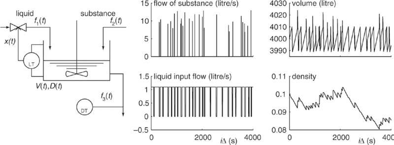
Figure 5.1 A density control system for the process industry.
If the transition probability density p(x(i + 1)|x(i)) is known together with the initial probability density p(x(0)), then the probability density at an arbitrary time can be determined recursively:
The joint probability density of the sequence x(0), x(1), …, x(i) follows readily:

5.1.1.2 The Measurement Model
Unfortunately in most cases we cannot directly observe the system states. Instead we can only observe the system outputs such as the data from the sensor in relation to the state. This means, in addition to the state space model, we also need a measurement model that describes the data from the system output. Suppose that at moment i the measurement data are z(i) ∈ Z, where Z is the measurement space. For the real-valued state variables, the measurement space is often a real-valued vector space, that is ![]() for some positive integer n. For the discrete case, one often assumes that the measurement space is also discrete. The measurement model is described by
for some positive integer n. For the discrete case, one often assumes that the measurement space is also discrete. The measurement model is described by
where v(i) is the measurement noise.
The probabilistic model of the measurement system is fully defined by the conditional probability density p(z(i)|x(0), …, x(i), z(0), …, z(i − 1)). We assume that the sequence of measurements starts at time i = 0. In order to shorten the notation, the sequence of all measurements up to the present will be denoted by
We restrict ourselves to memoryless measurement systems which is systems where z(i) depends on the value of x(i), but not on previous states nor on previous measurements. In other words:
The state model (5.1) together with the measurement model (5.8) forms the general discrete-time state space model for state estimation. However, this general model is not very useful until we move to more specific situations, which will be discussed later in this chapter.
5.1.2 Optimal Online Estimation
Figure 5.2 presents an overview of the scheme for the online estimation of the state. The connotation of the phrase online is that for each time index i an estimate ![]() of x(i) is produced based on Z(i), that is, based on all measurements that are available at that time. The crux of optimal online estimation is to maintain the posterior density p(x(i)|Z(i)) for running values of i. This density captures all the available information of the current state x(i) after having observed the current measurement and all previous ones. With the availability of the posterior density, the methods discussed in Chapters 3 and 4 become applicable. The only work to be done, then, is to adopt an optimality criterion and to work this out using the posterior density to get the optimal estimate of the current state.
of x(i) is produced based on Z(i), that is, based on all measurements that are available at that time. The crux of optimal online estimation is to maintain the posterior density p(x(i)|Z(i)) for running values of i. This density captures all the available information of the current state x(i) after having observed the current measurement and all previous ones. With the availability of the posterior density, the methods discussed in Chapters 3 and 4 become applicable. The only work to be done, then, is to adopt an optimality criterion and to work this out using the posterior density to get the optimal estimate of the current state.

Figure 5.2 An overview of online estimation.
The maintenance of the posterior density is done efficiently by means of a recursion. From the posterior density p(x(i)|Z(i)), valid for the current period i, the density p(x(i + 1)|Z(i + 1)), valid for the next period i + 1, is derived. The first step of the recursion cycle is a prediction step. The knowledge about x(i) is extrapolated to the knowledge about x(i + 1). Using Bayes’ theorem for conditional probabilities in combination with the Markov condition (5.2), we have

At this point, we increment the counter i so that p(x(i + 1)|Z(i)) now becomes p(x(i)|Z(i − 1). The increment can be done anywhere in the loop, but the choice to do it at this point leads to a shorter notation of the second step.
The second step is an update step. The knowledge gained from observing the measurement z(i) is used to refine the density. Using – once again – the theorem of Bayes, now in combination with the conditional density for memoryless sensory systems (5.9), gives

where c is a normalization constant:

The recursion starts with the processing of the first measurement z(0). The posterior density p(x(0)|Z(0)) is obtained using p(x(0)) as the prior.
The outline for optimal estimation, expressed in Equations (5.10), (5.11) and (5.12), is useful in the discrete case (where integrals turn into summations). For continuous states, a direct implementation is difficult for two reasons:
- It requires efficient representations for the multidimensional density functions.
- It requires efficient algorithms for the integrations over a multidimensional space.
Both requirements are hard to fulfil, especially if m is large. Nonetheless, many researchers have tried to implement the general scheme. One of the most successful endeavours has resulted in what is called particle filtering. First, however, the discussion will be focused on special cases.
5.2 Infinite Discrete-Time State Variables
As addressed in the last section, for continuous states a direct implementation is difficult. In order to overcome this difficulty, the continuous-time models are converted to infinite discrete-time models by reducing the continuous time to a sequence of specific times. The starting point is the general scheme for online estimation discussed in the previous section and illustrated in Figure 5.2. Suppose that both the state and the measurements are discrete real-valued vectors with dimensions of m and n, respectively. As stated before, in general a direct implementation of the scheme is still difficult even if the variables are discrete-time. Fortunately, there are circumstances that allow a fast implementation. For instance, in the special case, where the models are linear and the disturbances have a normal distribution, an implementation based on an ‘expectation and covariance matrix’ representation of the probability densities is feasible (Section 5.2.1). If the models are non-linear, but the non-linearity is smooth, linearization techniques can be applied (Section 5.2.2). If the models are highly non-linear but the dimensions m and n are not too large, numerical methods are possible (Sections 5.4 and 5.5).
5.2.1 Optimal Online Estimation in Linear-Gaussian Systems
Most literature in optimal estimation in dynamic systems deals with the particular case in which both the state model and the measurement model are linear, and the disturbances are Gaussian (the linear-Gaussian systems). Perhaps the main reason for the popularity is the mathematical tractability of this case.
5.2.1.1 Linear-Gaussian State Space Models
The state model is said to be linear if the state space model (5.1) can be expressed by a so-called linear system equation (or linear state equation, linear plant equation, linear dynamic equation):
where F(i) is the system matrix. It is an m × m matrix where m is the dimension of the state vector; m is called the order of the system. The vector u(i) is the control vector (input vector) of dimension l. Usually, the vector is generated by a controller according to some control law. As such the input vector is a deterministic signal that is fully known, at least up to the present. L(i) is the gain matrix of dimension m × l. Sometimes the matrix is called the distribution matrix as it distributes the control vector across the elements of the state vector.
w(i) is the process noise (system noise, plant noise). It is a sequence of random vectors of dimension m. The process noise represents the unknown influences on the system, for instance, formed by disturbances from the environment. The process noise can also represent an unknown input/control signal. Sometimes process noise is also used to take care of modelling errors. The general assumption is that the process noise is a white random sequence with normal distribution. The term ‘white’ is used here to indicate that the expectation is zero and the autocorrelation is governed by the Kronecker delta function:

where Cw(i) is the covariance matrix of w(i). Since w(i) is supposed to have a normal distribution with zero mean, Cw(i) defines the density of w(i) in full.
The initial condition of the state model is given in terms of the expectation E[x(0)] and the covariance matrix Cx(0). In order to find out how these parameters of the process propagate to an arbitrary time i, the state equation (5.13) must be used recursively:

The first equation follows from E[w(i)] = 0. The second equation uses the fact that the process noise is white, that is E[w(i)wT(j)] = 0 for i ≠ j (see Equation (5.14)).
If E[x(0)] and Cx(0) are known, then Equation (5.15) can be used to calculate E[x(1)] and Cx(1). From that, by reapplying (5.15), the next values, E[x(2)] and Cx(2), can be found, and so on. Thus, the iterative use of Equation (5.15) gives us E[x(i)] and Cx(i) for arbitrary i > 0.
In the special case, where neither F(i) nor C(i) depends on i, the state space model is time invariant. The notation can then be shortened by dropping the index, that is F and Cw. If, in addition, F is stable (i.e. the magnitudes of the eigenvalues of F are all less than one), the sequence Cx(i), i = 0, 1, … converges to a constant matrix. The balance in Equation (5.15) is reached when the decrease of Cx(i) due to F compensates for the increase of Cx(i) due to Cw. If such is the case, then
which is the discrete Lyapunov equation.
5.2.1.2 Prediction
Equation (5.15) is the basis for prediction. Suppose that at time i an unbiased estimate ![]() is known together with the associated error covariance Ce(i), which was introduced in Section 4.2.2. The best predicted value (MMSE) of the state for ℓ samples ahead of i is obtained by the recursive application of Equation (5.15). The recursion starts with
is known together with the associated error covariance Ce(i), which was introduced in Section 4.2.2. The best predicted value (MMSE) of the state for ℓ samples ahead of i is obtained by the recursive application of Equation (5.15). The recursion starts with ![]() and terminates when E[x(i + ℓ)] is obtained. The covariance matrix Ce(i) is a measure of the magnitudes of the random fluctuations of x(i) around
and terminates when E[x(i + ℓ)] is obtained. The covariance matrix Ce(i) is a measure of the magnitudes of the random fluctuations of x(i) around ![]() . As such it is also a measure of uncertainty. Therefore, the recursive usage of Equation (5.15) applied to Ce(i) gives Ce(i + ℓ), that is the uncertainty of the prediction. With that, the recursive equations for the prediction become
. As such it is also a measure of uncertainty. Therefore, the recursive usage of Equation (5.15) applied to Ce(i) gives Ce(i + ℓ), that is the uncertainty of the prediction. With that, the recursive equations for the prediction become

Example 5.3 Prediction of motion tracking Example 5.1 formulated a simple motion tracking problem with the state equation (5.4), where

and
According to Equation (5.17), the one step ahead prediction (ℓ = 0) can be expressed as
where ![]() represents the input term. The prediction error covariance at the time i is
represents the input term. The prediction error covariance at the time i is
where ![]() is the covariance of
is the covariance of ![]() , which is
, which is

if ![]() is a white random sequence. Suppose the initial prediction error covariance is 0, that is
is a white random sequence. Suppose the initial prediction error covariance is 0, that is

Then ![]() can be generated recursively according to Equation (5.19). By Equation (5.4),
can be generated recursively according to Equation (5.19). By Equation (5.4), ![]() can be set to 0. Also suppose the sample interval is 1, that is
can be set to 0. Also suppose the sample interval is 1, that is

This example will be extended to a complete example of online estimation with a discrete Kalman filter by establishing the measurement model in Example 5.4.
5.2.1.3 Linear-Gaussian Measurement Models
A special form of Equation (5.8) is the linear measurement model, which takes the following form:
where H(i) is the so-called measurement matrix, which is an n × m matrix and v(i) is the measurement noise. It is a sequence of random vectors of dimension n. Obviously, the measurement noise represents the noise sources in the sensory system. Examples are thermal noise in a sensor and the quantization errors of an AD converter.
The general assumption is that the measurement noise is a zero mean, white random sequence with normal distribution. In addition, the sequence is supposed to have no correlation between the measurement noise and the process noise:

where Cv(i) is the covariance matrix of v(i). Cv(i) specifies the density of v(i) in full.
The measurement system is time invariant if neither H nor Cv depends on i.
5.2.1.4 The Discrete Kalman Filter
The concepts developed in the previous section are sufficient to transform the general scheme presented in Section 5.1 into a practical solution. In order to develop the estimator, first the initial condition valid for i = 0 must be established. In the general case, this condition is defined in terms of the probability density p(x(0)) for x(0). Assuming a normal distribution for x(0) it suffices to specify only the expectation E[x(0)] and the covariance matrix Cx(0). Hence, the assumption is that these parameters are available. If not, we can set E[x(0)] = 0 and let Cx(0) approach infinity, that is Cx(0) → ∞ I. Such a large covariance matrix represents the lack of prior knowledge.
The next step is to establish the posterior density p(x(0)|z(0)) from which the optimal estimate for x(0) follows. At this point, we enter the loop of Figure 5.2. Hence, we calculate the density p(x(1)|z(0)) of the next state and process the measurement z(1) resulting in the updated density p(x(1)|z(0), z(1)) = p(x(1)|Z(1)). From that, the optimal estimate for x(1) follows. This procedure has to be iterated for all of the next time cycles.
The representation of all the densities that are involved can be given in terms of expectations and covariances. The reason is that any linear combination of Gaussian random vectors yields a vector that is also Gaussian. Therefore, both p(x(i + 1)|Z(i)) and p(x(i)|Z(i)) are fully represented by their expectations and covariances. In order to discriminate between the two situations a new notation is needed. From now on, the conditional expectation E[x(i)|Z(j)] will be denoted by ![]() . It is the expectation associated with the conditional density p(x(i)|Z(j)). The covariance matrix associated with this density is denoted by C(i|j).
. It is the expectation associated with the conditional density p(x(i)|Z(j)). The covariance matrix associated with this density is denoted by C(i|j).
The update, that is the determination of p(x(i)|Z(i)) given p(x(i)|Z(i − 1)), follows from Section 4.1.5, where it has been shown that the unbiased linear MMSE estimate in the linear-Gaussian case equals the MMSE estimate, and that this estimate is the conditional expectation. Application of Equations (4.33) and (4.45) to (5.20) and (5.21) gives

The interpretation is as follows: ![]() is the predicted measurement. It is an unbiased estimate of z(i) using all information from the past. The so-called innovation matrix S(i) represents the uncertainty of the predicted measurement. The uncertainty is due to two factors: the uncertainty of x(i) as expressed by C(i|i − 1) and the uncertainty due to the measurement noise v(i) as expressed by Cv(i). The matrix K(i) is the Kalman gain matrix. This matrix is large when S(i) is small and C(i|i − 1)HT(i) is large, that is when the measurements are relatively accurate. When this is the case, the values in the error covariance matrix C(i|i) will be much smaller than C(i|i − 1).
is the predicted measurement. It is an unbiased estimate of z(i) using all information from the past. The so-called innovation matrix S(i) represents the uncertainty of the predicted measurement. The uncertainty is due to two factors: the uncertainty of x(i) as expressed by C(i|i − 1) and the uncertainty due to the measurement noise v(i) as expressed by Cv(i). The matrix K(i) is the Kalman gain matrix. This matrix is large when S(i) is small and C(i|i − 1)HT(i) is large, that is when the measurements are relatively accurate. When this is the case, the values in the error covariance matrix C(i|i) will be much smaller than C(i|i − 1).
The prediction, that is the determination of p(x(i + 1)|Z(i)) given p(x(i)|Z(i)), boils down to finding out how the expectation ![]() and the covariance matrix C(i|i) propagate to the next state. Using equations (5.13) and (5.15) we have
and the covariance matrix C(i|i) propagate to the next state. Using equations (5.13) and (5.15) we have

At this point, we increment the counter and x(i + 1|i) and C(i + 1|i) become x(i|i − 1) and C(i|i − 1). These recursive equations are generally referred to as the discrete Kalman filter (DKF).
In the Gaussian case, it does not matter much which optimality criterion we select. MMSE estimation, MMAE estimation and MAP estimation yield the same result, that is the conditional mean. Hence, the final estimate is found as ![]() . It is an absolute unbiased estimate and its covariance matrix is C(i|i). Therefore, this matrix is often called the error covariance matrix.
. It is an absolute unbiased estimate and its covariance matrix is C(i|i). Therefore, this matrix is often called the error covariance matrix.
In the time invariant case, and assuming that the Kalman filter is stable, the error covariance matrix converges to a constant matrix. In that case, the innovation matrix and the Kalman gain matrix become constant as well. The filter is said to be in the steady state. The steady state condition simply implies that C(i + 1|i) = C(i|i − 1). If the notation for this matrix is shortened to P, then Equations (5.22) and (5.23) lead to the following equation:
Equation (5.24) is known as the discrete algebraic Ricatti equation. Usually, it is solved numerically. Its solution implicitly defines the steady state solution for S, K and C.
Example 5.4 Application to the motion tracking In this example we reconsider the motion tracking described in Example 5.3. We model the measurements with the model: ![]() where
where ![]() is the constant matrix
is the constant matrix

Figure 5.3 shows the results of the motion tracking. The covariance of the measurement noise is ![]() . The filter is initiated with
. The filter is initiated with ![]() to be the actual position of the object. Recall that in Example 5.3, Cx(0) is set to be 1. It can be seen from Figure 5.3 that if both system error and measurement error are white noise with covariance 1, the motion tracking works quite well.
to be the actual position of the object. Recall that in Example 5.3, Cx(0) is set to be 1. It can be seen from Figure 5.3 that if both system error and measurement error are white noise with covariance 1, the motion tracking works quite well.

Figure 5.3 Motion tracking: both system and measurement errors are white noises with covariance 1.
Listing 5.1 is the code of this example.
Listing 5.1 Discrete Kalman filter for motion tracking
clear
x=(1:80);
for idx = 1: length(x)
 y(idx)=(idx-22)*(idx-22)/20;
end
y=2*randn(1,length(x)) + y;

kalman = [];
for idx = 1: length(x)
   location = [x(idx),y(idx),0,0];
   if isempty(kalman)
       stateModel = [1 0 1 0;0 1 0 1;0 0 1 0;0 0 0 1];
       measurementModel = [1 0 0 0;0 1 0 0;0 0 1 0;0 0 0 1];
       kalman = vision.KalmanFilter(stateModel,measurementModel,
       'ProcessNoise',1,'MeasurementNoise',1);
       kalman.State = location;
   else
       trackedLocation = predict(kalman);
       plot(location(1),location(2),'k+');
       trackedLocation = correct(kalman,location);
       pause(0.2);
       plot(trackedLocation(1),trackedLocation(2),'ro');
   end
end
For comparison, Figure 5.4 depicts the tracking results when the system noise becomes 1 × 10⁻⁴ (=0.0001) while the measurement noise becomes 4. This time the performance is much worse after time step 28.

Figure 5.4 Motion tracking: measurement errors are white noise with covariance 4.
5.2.2 Suboptimal Solutions for Non-linear Systems
This section extends the discussion on state estimation to the more general case of non-linear systems and non-linear measurement functions:

The vector f( ·, ·, ·) is a non-linear, time variant function of the state x(i) and the control vector u(i). The control vector is a deterministic signal. Since u(i) is fully known, it only causes an explicit time dependency in f( ·, ·, ·). Without loss of generality, the notation can be shortened to f(x(i), i) because such an explicit time dependency is already implied in that shorter notation. If no confusion can occur, the abbreviation f(x(i)) will be used instead of f(x(i), i) even if the system does depend on time. As before, w(i) is the process noise. It is modelled as zero mean, Gaussian white noise with covariance matrix Cw(i). The vector h( ·, ·) is a nonlinear measurement function. Here too, if no confusion is possible, the abbreviation h(x(i)) will be used covering both the time variant and the time invariant case. v(i) represents the measurement noise, modelled as zero mean, Gaussian white noise with covariance matrix Cv(i).
Any Gaussian random vector that undergoes a linear operation retains its Gaussian distribution. A linear operator only affects the expectation and the covariance matrix of that vector. This property is the basis of the Kalman filter. It is applicable to linear-Gaussian systems and it permits a solution that is entirely expressed in terms of expectations and covariance matrices. However, the property does not hold for non-linear operations. In non-linear systems, the state vectors and the measurement vectors are not Gaussian distributed, even though the process noise and the measurement noise might be. Consequently, the expectation and the covariance matrix do not fully specify the probability density of the state vector. The question is then how to determine this non-Gaussian density and how to represent it in an economical way. Unfortunately, no general answer exists to this question.
This section seeks the answer by assuming that the non-linearities of the system are smooth enough to allow linear or quadratic approximations. Using these approximations, Kalman-like filters become within reach. These solutions are suboptimal since there is no guarantee that the approximations are close.
An obvious way to get the approximations is by application of a Taylor series expansion of the functions. Ignorance of the higher-order terms of the expansion gives the desired approximation. The Taylor series exists by virtue of the assumed smoothness of the non-linear function; it does not work out if the non-linearity is a discontinuity, that is saturation, dead zone, hysteresis, and so on. The Taylor series expansions of the system equations are as follows:

where ei is the Cartesian basis vector with appropriate dimension. The ith element of ei is one; the others are zeros; ei can be used to select the ith element of a vector: eTix = xi. F(x) and H(x) are Jacobian matrices. Fixx(x) and Hjxx(x) are Hessian matrices. These matrices are defined in Appendix B.4. HOT are the higher-order terms. The quadratic approximation arises if the higher-order terms are ignored. If, in addition, the quadratic term is ignored, the approximation becomes linear, e.g. ![]() .
.
5.2.2.1 The Linearized Kalman Filter
The simplest approximation occurs when the system equations are linearized around some fixed value ![]() of x(i). This approximation is useful if the system is time invariant and stable, and if the states swing around an equilibrium state. Such a state is the solution of
of x(i). This approximation is useful if the system is time invariant and stable, and if the states swing around an equilibrium state. Such a state is the solution of
Defining ![]() , the linear approximation of the state equation (5.25) becomes
, the linear approximation of the state equation (5.25) becomes ![]() . After some manipulations:
. After some manipulations:

By interpreting the term ![]() as a constant control input and by compensating the offset term
as a constant control input and by compensating the offset term ![]() in the measurement vector, these equations become equivalent to Equations (5.13) and (5.20). This allows the direct application of the DKF as given in Equations (5.22) and (5.23).
in the measurement vector, these equations become equivalent to Equations (5.13) and (5.20). This allows the direct application of the DKF as given in Equations (5.22) and (5.23).
Many practical implementations of the discrete Kalman filter are inherently linearized Kalman filters because physical processes are seldom exactly linear and often a linear model is only an approximation of the real process.
Example 5.5 A linearized model for volume density estimation In Section 5.1.1 we introduced the non-linear, non-Gaussian problem of the volume density estimation of a mix in the process industry (Example 5.2). The model included a discrete state variable to describe the on/off regulation of the input flow. We will now replace this model by a linear feedback mechanism:

The liquid input flow has now been modelled by f1(i) = α(V0 − V(i)) + w1(i). The constant V0 = Vref + (c − f2)/α (with ![]() realizes the correct mean value of V(i). The random part w1(i) of f1(i) establishes a first-order AR model of V(i), which is used as a rough approximation of the randomness of f1(i). The substance input flow f2(i), which in Example 5.2 appears as chunks at some discrete points of time, is now modelled by
realizes the correct mean value of V(i). The random part w1(i) of f1(i) establishes a first-order AR model of V(i), which is used as a rough approximation of the randomness of f1(i). The substance input flow f2(i), which in Example 5.2 appears as chunks at some discrete points of time, is now modelled by ![]() , that is a continuous flow with some randomness.
, that is a continuous flow with some randomness.
The equilibrium is found as the solution of V(i + 1) = V(i) and D(i + 1) = D(i). The results are

The expressions for the Jacobian matrices are

The considered measurement system consists of two sensors:
- A level sensor that measures the volume V(i) of the barrel.
- A radiation sensor that measures the density D(i) of the output flow.
The latter uses the radiation of some source, for example X-rays, that is absorbed by the fluid. According to Beer–Lambert's law, Pout = Pinexp ( − μD(i)), where μ is a constant depending on the path length of the ray and on the material. Using an optical detector the measurement function becomes z = Uexp ( − μD) + v with U a constant voltage. With that, the model of the two sensors becomes

with the Jacobian matrix:

The best fitted parameters of this model are as follows:
| Volume | Substance | Output | Measurement |
| control | flow | flow | system |
| Δ = 1 (s) | Vref = 4000 (l) | ||
| V0 = 4001 (l) | c = 1 (l/s) | U = 1000 (V) | |
| α = 0.95 (1/s) | μ = 100 | ||
Figure 5.5 shows the real states (obtained from a simulation using the model from Example 5.2), observed measurements, estimated states and estimation errors. It can be seen that:
- The density can only be estimated if the real density is close to the equilibrium. In every other region, the linearization of the measurement is not accurate enough.
- The estimator is able to estimate the mean volume but cannot keep track of the fluctuations. The estimation error of the volume is much larger than indicated by the 1σ boundaries (obtained from the error covariance matrix). The reason for the inconsistent behaviour is that the linear-Gaussian AR model does not fit well enough.

Figure 5.5 Linearized Kalman filtering applied to the volume density estimation problem.
5.2.2.2 The Extended Kalman Filter
A straightforward generalization of the linearized Kalman filter occurs when the equilibrium point ![]() is replaced with a nominal trajectory
is replaced with a nominal trajectory ![]() , recursively defined as
, recursively defined as
Although the approach is suitable for time variant systems, it is not often used. There is another approach with almost the same computational complexity, but with better performance. That approach is the extended Kalman filter (EKF).
Again, the intention is to keep track of the conditional expectation x(i|i) and the covariance matrix C(i|i). In the linear-Gaussian case, where all distributions are Gaussian, the conditional mean is identical to the MMSE estimate (= minimum variance estimate), the MMAE estimate and the MAP estimate (see Section 4.1.3). In the present case, the distributions are not necessarily Gaussian and the solutions of the three estimators do not coincide. The extended Kalman filter provides only an approximation of the MMSE estimate.
Each cycle of the extended Kalman filter consists of a ‘one step ahead’ prediction and an update, as before. However, the tasks are much more difficult now because the calculation of, for instance, the ‘one step ahead’ expectation:
requires the probability density p(x(i + 1)|Z(i)) (see Equation (5.10)). However, as stated before, it is not clear how to represent this density. The solution of the EKF is to apply a linear approximation of the system function. With that, the ‘one step ahead’ expectation can be expressed entirely in terms of the moments of p(x(i)|Z(i)).
The EKF uses linear approximations of the system functions using the first two terms of the Taylor series expansions. Suppose that at time i we have the updated estimate ![]() and the associated approximate error covariance matrix C(i|i). The word ‘approximate’ expresses the fact that our estimates are not guaranteed to be unbiased due to the linear approximations. However, we do assume that the influence of the errors induced by the linear approximations is small. If the estimation error is denoted by e(i), then
and the associated approximate error covariance matrix C(i|i). The word ‘approximate’ expresses the fact that our estimates are not guaranteed to be unbiased due to the linear approximations. However, we do assume that the influence of the errors induced by the linear approximations is small. If the estimation error is denoted by e(i), then

In these expressions, ![]() is our estimate. It is available at time i and therefore is deterministic. Only e(i) and w(i) are random. Taking the expectation on both sides of (5.28), we obtain approximate values for the ‘one step ahead’ prediction:
is our estimate. It is available at time i and therefore is deterministic. Only e(i) and w(i) are random. Taking the expectation on both sides of (5.28), we obtain approximate values for the ‘one step ahead’ prediction:
We have approximations instead of equalities for two reasons. First, we neglect the possible bias of ![]() , that is a non-zero mean of e(i). Second, we ignore the higher-order terms of the Taylor series expansion.
, that is a non-zero mean of e(i). Second, we ignore the higher-order terms of the Taylor series expansion.
Upon incrementing the counter, ![]() becomes
becomes ![]() and we now have to update the prediction
and we now have to update the prediction ![]() by using a new measurement z(i) in order to get an approximation of the conditional mean
by using a new measurement z(i) in order to get an approximation of the conditional mean ![]() . First we calculate the predicted measurement
. First we calculate the predicted measurement ![]() based on
based on ![]() using a linear approximation of the measurement function, that is
using a linear approximation of the measurement function, that is ![]() . Next, we calculate the innovation matrix S(i) using that same approximation. Then we apply the update according to the same equations as in the linear-Gaussian case.
. Next, we calculate the innovation matrix S(i) using that same approximation. Then we apply the update according to the same equations as in the linear-Gaussian case.
The predicted measurements are

The approximation is based on the assumption that E[e(i|i − 1)]≅0 and on the Taylor series expansion of h( · ). The innovation matrix becomes
From this point on, the update continues as in the linear-Gaussian case (see Equation (5.22)):

Despite the similarity of the last equation with respect to the linear case, there is an important difference. In the linear case, the Kalman gain K(i) depends solely on deterministic parameters: H(i), F(i), Cw(i), Cv(i) and Cx(0). It does not depend on the data. Therefore, K(i) is fully deterministic. It could be calculated in advance instead of online. In the EKF, the gains depend upon the estimated states ![]() through
through ![]() , and thus also upon the measurements z(i). Therefore, the Kalman gains are random matrices. Two runs of the extended Kalman filter in two repeated experiments lead to two different sequences of the Kalman gains. In fact, this randomness of K(i) can cause unstable behaviour.
, and thus also upon the measurements z(i). Therefore, the Kalman gains are random matrices. Two runs of the extended Kalman filter in two repeated experiments lead to two different sequences of the Kalman gains. In fact, this randomness of K(i) can cause unstable behaviour.
Example 5.6 The extended Kalman filter for volume density estimation Application of the EKF to the density estimation problem introduced in Example 5.2 and represented by a linear-Gaussian model in Example 5.5 gives the results as shown in Figure 5.6. Compared with the results of the linearized KF (Figure 5.5) the density errors are now much more consistent with the 1σ boundaries obtained from the error covariance matrix. However, the EKF is still not able to cope with the non-Gaussian disturbances of the volume.
Note also that the 1σ boundaries do not reach a steady state. The filter remains time variant, even in the long term.

Figure 5.6 Extended Kalman filtering for the volume density estimation problem.
5.2.2.3 The Iterated Extended Kalman Filter
A further improvement of the update step in the extended Kalman filter is within reach if the current estimate ![]() is used to get an improved linear approximation of the measurement function yielding an improved predicted measurement
is used to get an improved linear approximation of the measurement function yielding an improved predicted measurement ![]() . In turn, such an improved predicted measurement can improve the current estimate. This suggests an iterative approach.
. In turn, such an improved predicted measurement can improve the current estimate. This suggests an iterative approach.
Let ![]() be the predicted measurement in the ℓth iteration and let
be the predicted measurement in the ℓth iteration and let ![]() be the ℓth improvement of
be the ℓth improvement of ![]() . The iteration is initiated with
. The iteration is initiated with ![]() . A naive approach for the calculation of
. A naive approach for the calculation of ![]() simply uses a relinearization of h( · ) based on
simply uses a relinearization of h( · ) based on ![]() :
:

Hopefully, the sequence ![]() , with ℓ = 0, 1, 2, …, converges to a final solution.
, with ℓ = 0, 1, 2, …, converges to a final solution.
A better approach is the so-called iterated extended Kalman filter (IEKF). Here, the approximation is made that both the predicted state and the measurement noise are normally distributed. With that, the posterior probability density (Equation (5.11))
being the product of two Gaussians, is also a Gaussian. Thus, the MMSE estimate coincides with the MAP estimate and the task is now to find the maximum of p(x(i)|Z(i)). Equivalently, we maximize its logarithm. After the elimination of the irrelevant constants and factors, it all boils down to minimizing the following function w.r.t. x:
For brevity, the following notation has been used:

The strategy to find the minimum is to use the Newton–Raphson iteration starting from ![]() . In the ℓth iteration step, we already have an estimate
. In the ℓth iteration step, we already have an estimate ![]() obtained from the previous step. We expand f(x) in a second-order Taylor series approximation:
obtained from the previous step. We expand f(x) in a second-order Taylor series approximation:

where ∂f/∂x is the gradient and ∂2f/∂x2 is the Hessian of f(x) (see Appendix B.4). The estimate ![]() is the minimum of the approximation. It is found by equating the gradient of the approximation to zero. Differentiation of Equation (5.30) w.r.t. x gives
is the minimum of the approximation. It is found by equating the gradient of the approximation to zero. Differentiation of Equation (5.30) w.r.t. x gives

The Jacobian and Hessian of Equation (5.29), in explicit form, are

where ![]() is the Jacobian matrix of h(x) evaluated at
is the Jacobian matrix of h(x) evaluated at ![]() . Substitution of Equation (5.32) in (5.31) yields the following iteration scheme:
. Substitution of Equation (5.32) in (5.31) yields the following iteration scheme:

The result after one iteration, that is ![]() , is identical to the ordinary extended Kalman filter. The required number of further iterations depends on how fast
, is identical to the ordinary extended Kalman filter. The required number of further iterations depends on how fast ![]() converges. Convergence is not guaranteed, but if the algorithm converges, usually a small number of iterations suffice. Therefore, it is common practice to fix the number of iterations to some practical number L. The final result is set to the last iteration, that is
converges. Convergence is not guaranteed, but if the algorithm converges, usually a small number of iterations suffice. Therefore, it is common practice to fix the number of iterations to some practical number L. The final result is set to the last iteration, that is ![]() .
.
Equation (4.44) shows that the factor (C− 1p + HℓTC− 1vHℓ)− 1 is the error covariance matrix associated with x(i|i):
This insight gives another connotation to the last term in Equation (5.33) because, in fact, the term C(i|i)HTℓCv− 1 can be regarded as the Kalman gain matrix Kℓ during the ℓth iteration (see Equation (4.20)).
Example 5.7 The iterated EKF for volume density estimation In the previous example, the EKF was applied to the density estimation problem introduced in Example 5.2. The filter was initiated with the equilibrium state as prior knowledge, that is ![]() . Figure 5.7(b) shows the transient that occurs if the EKF is initiated with E[x(0)] = [2000 0]T. It takes about 40(s) before the estimated density reaches the true densities. This slow transient is due to the fact that in the beginning the linearization is poor. The iterated EKF is of much help here. Figure 5.7(c) shows the results. From the first measurement, the estimated density is close to the real density. There is no transient.
. Figure 5.7(b) shows the transient that occurs if the EKF is initiated with E[x(0)] = [2000 0]T. It takes about 40(s) before the estimated density reaches the true densities. This slow transient is due to the fact that in the beginning the linearization is poor. The iterated EKF is of much help here. Figure 5.7(c) shows the results. From the first measurement, the estimated density is close to the real density. There is no transient.

Figure 5.7 Iterated extended Kalman filtering for the volume density estimation problem. (a) Measurements. (b) Results from the EKF. (c) Results from the iterated EKF (number of iterations = 20).
The extended Kalman filter is widely used because for a long period of time no viable alternative solution existed. Nevertheless, it has numerous disadvantages:
- It only works well if the various random vectors are approximately Gaussian distributed. For complicated densities, the expectation–covariance representation does not suffice.
- It only works well if the non-linearities of the system are not too severe because otherwise the Taylor series approximations fail. Discontinuities are deadly for the EKF's proper functioning.
- Recalculating the Jacobian matrices at every time step is computationally expensive.
- In some applications, it is too difficult to find the Jacobian matrix analytically. In these cases, numerical approximations of the Jacobian matrix are needed. However, this introduces other types of problems because now the influence of having approximations rather than the true values comes in.
- In the EKF, the Kalman gain matrix depends on the data. With that, the stability of the filter is no longer assured. Moreover, it is very hard to analyse the behaviour of the filter.
- The EKF does not guarantee unbiased estimates. In addition, the calculated error covariance matrices do not necessarily represent the true error covariances. The analysis of these effects is also hard.
5.3 Finite Discrete-Time State Variables
We consider physical processes that are described at any time as being in one of a finite number of states. Examples of such processes are:
- The sequence of strokes of a tennis player during a game, for example service, backhand-volley, smash, etc.
- The sequence of actions that a tennis player performs during a particular stroke.
- The different types of manoeuvres of an airplane, for example a linear flight, a turn, a nose dive, etc.
- The sequence of characters in a word and the sequence of words in a sentence.
- The sequence of tones of a melody as part of a musical piece.
- The emotional modes of a person: angry, happy, astonished, etc.
These situations are described by a state variable x(i) that can only take a value from a finite set of states Ω = {ω1, …, ωK}.
The task is to determine the sequence of states that a particular process goes through (or has gone through). For that purpose, at any time measurements z(i) are available. Often the output of the sensors is real valued, but nevertheless we will assume that the measurements take their values from a finite set. Thus, some sort of discretization must take place that maps the range of the sensor data on to a finite set Z = {ϑ1, …, ϑN}.
This section first introduces a state space model that is often used for discrete state variables, that is the hidden Markov model. This model will be used in the next subsections for online and offline estimation of the states.
5.3.1 Hidden Markov Models
A hidden Markov model (HMM) is an instance of the state space model discussed in Section 5.1.1. It describes a sequence x(i) of discrete states starting at time i = 0. The sequence is observed by means of measurements z(i) that can only take values from a finite set. The model consists of the following ingredients:
- The set Ω containing the K states ωk that x(i) can take.
- The set Z containing the N symbols ϑn that z(i) can take.
- The initial state probability p0(x(0)).
- The state transition probability pt(x(i)|x(i − 1)).
- The observation probability pz(z(i)|x(i)).
The expression p0(x(0)) with x(0) ∈ {1, …, K} denotes the probability that the random state variable ![]() takes the value ωx(0). Thus
takes the value ωx(0). Thus ![]() . Similar conventions hold for other expressions, like pt(x(i)|x(i − 1)) and pz(z(i)|x(i)).
. Similar conventions hold for other expressions, like pt(x(i)|x(i − 1)) and pz(z(i)|x(i)).
The Markov condition of an HMM states that p(x(i)|x(0), …, x(i − 1)), that is the probability of x(i) under the condition of all previous states, equals the transition probability. The assumption of the validity of the Markov condition leads to a simple, yet powerful model. Another assumption of the HMM is that the measurements are memoryless. In other words, z(i) only depends on x(i) and not on the states at other time points: p(z(j)|x(0), …, x(i)) = p(z(j)|x(j)).
An ergodic Markov model is one for which the observation of a single sequence x(0), x(1), …, x(∞) suffices to determine all the state transition probabilities. A suitable technique for that is histogramming, that is the determination of the relative frequency with which a transition occurs (see Section 6.2.5). A sufficient condition for ergodicity is that all state probabilities are non-zero. In that case, all states are reachable from everywhere within one time step. Figure 5.8 is an illustration of an ergodic model.

Figure 5.8 A three-state ergodic Markov model.
Another type is the so-called left–right model (see Figure 5.9). This model has the property that the state index k of a sequence is non-decreasing as time proceeds. Such is the case when pt(k|ℓ) = 0 for all k < l. In addition, the sequence always starts with ω1 and terminates with ωK. Thus, p0(k) = δ(k, 1) and pt(k|K) = δ(k, K). Sometimes, an additional constraint is that large jumps are forbidden. Such a constraint is enforced by letting pt(k|ℓ) = 0 for all k > ℓ + Δ. Left–right models find applications in processes where the sequence of states must obey some ordering over time. An example is the stroke of a tennis player. For instance, the service of the player follows a sequence like: ‘take position behind the base line’, ‘bring racket over the shoulder behind the back’, ‘bring up the ball with the left arm’, etc.

Figure 5.9 A four-state left–right model.
In a hidden Markov model the state variable x(i) is observable only through its measurements z(i). Now, suppose that a sequence Z(i) = {z(0), z(1), …, z(i)} of measurements has been observed. Some applications require the numerical evaluation of the probability p(Z(i)) of a particular sequence. An example is the recognition of a stroke of a tennis player. We can model each type of stroke by an HMM that is specific for that type, thus having as many HMMs as the types of strokes. In order to recognize the stroke, we calculate for each type of stroke the probability p(Z(i)|type of stroke) and select the one with maximum probability.
For a given HMM and a fixed sequence Z(i) of acquired measurements, p(Z(i)) can be calculated by using the joint probability of having the measurements Z(i) together with a specific sequence of state variables, that is X(i) = {x(0), x(1), …, x(i)}. First we calculate the joint probability p(X(i), Z(i)):

where it is assumed that the measurement z(i) only depends on x(i). Then p(Z(i)) follows from summation over all possible state sequences:
Since there are Ki different state sequences, the direct implementation of Equations (5.34) and (5.35) requires on the order of (i + 1)Ki + 1 operations. Even for modest values of i, the number of operations is already impractical.
A more economical approach is to calculate p(Z(i)) by means of recursion. Consider the probability p(Z(i), x(i)). This probability can be calculated from the previous time step i − 1 using the following expression:

The recursion must be initiated with p(z(0), x(0)) = p0(x(0))pz(z(0)|x(0)). The probability p(Z(i)) can be retrieved from p(Z(i), x(i)) by

The so-called forward algorithm uses the array F(i, x(i)) = p(Z(i), x(i)) to implement the recursion.
Algorithm 5.1 The forward algorithm
- Initialization:

- Recursion:

- for x(i) = 1, …, K


- for x(i) = 1, …, K
In each recursion step, the sum consists of K terms and the number of possible values of x(i) is also K. Therefore, such a step requires on the order of K2 calculations. The computational complexity for i time steps is on the order of (i + 1)K2.
5.3.2 Online State Estimation
We now focus our attention on the situation of having a single HMM, where the sequence of measurements is processed online so as to obtain real-time estimates ![]() of the states. This problem completely fits within the framework of Section 5.1. Therefore, the solution provided by Equations (5.10) and (5.11) is valid, albeit that the integrals must be replaced by summations.
of the states. This problem completely fits within the framework of Section 5.1. Therefore, the solution provided by Equations (5.10) and (5.11) is valid, albeit that the integrals must be replaced by summations.
However, in line with the previous section, an alternative solution will be presented that is equivalent to the one in Section 5.1. The alternative solution is obtained by deduction of the posterior probability:
In view of the fact that Z(i) are the acquired measurements (and are known and fixed) the maximization of p(x(i)|Z(i)) is equivalent to the maximization of p(Z(i), x(i)). Therefore, the MAP estimate is found as
The probability p(Z(i), x(i)) follows from the forward algorithm.
Example 5.8 Online licence plate detection in videos This example demonstrates the ability of HMMs to find the licence plate of a vehicle in a video. Figure 5.10 is a typical example of one frame of such a video. The task is to find all the pixels that correspond to the licence plate. Such a task is the first step in a licence plate recognition system.
A major characteristic of video is that a frame is scanned line-by-line and that each video line is acquired from left to right. The real-time processing of each line individually is preferable because the throughput requirement of the application is demanding. Therefore, each line is individually modelled as an HMM. The hidden state of a pixel is determined by whether the pixel corresponds to a licence plate or not.
The measurements are embedded in the video line (see Figure 5.11). However, the video signal needs to be processed in order to map it on to a finite measurement space. Simply quantizing the signal to a finite number of levels does not suffice because the amplitudes of the signal alone are not very informative. The main characteristic of a licence plate in a video line is a typical pattern of dark–bright and bright–dark transitions due to the dark characters against a bright background, or vice versa. The image acquisition is such that the camera–object distance is about constant for all vehicles. Therefore, the statistical properties of the succession of transitions are typical for the imaged licence plate regardless of the type of vehicle.
One possibility to decode the succession of transitions is to apply a filter bank and to threshold the output of each filter, thus yielding a set of binary signals. In Figure 5.11, three high-pass filters have been applied with three different cut-off frequencies. Using high-pass filters has the advantage that the thresholds can be zero. Therefore, the results do not depend on the contrast and brightness of the image. The three binary signals define a measurement signal z(i) consisting of N = 8 symbols. Figure 5.12 shows these symbols for one video line. Here, the symbols are encoded as integers from 1 up to 8.
Due to the spatial context of the three binary signals we cannot model the measurements as memoryless symbols. The trick to avoid this problem is to embed the measurement z(i) in the state variable x(i). This can be done by encoding the state variable as integers from 1 up to 16. If i is not a licence plate pixel, we define the state as x(i) = z(i). If i is a licence plate pixel, we define x(i) = z(i) + 8. With that, K = 16. Figure 5.12 shows these states for one video line.

Figure 5.10 Licence plate detection.

Figure 5.11 Definitions of the measurements associated with a video line.

Figure 5.12 States and measurements of a video line.
The embedding of the measurements in the state variables is a form of state augmentation. Originally, the number of states was 2, but after this particular state augmentation, the number becomes 16. The advantage of the augmentation is that the dependence, which does exist between any pair z(i), z(j) of measurements, is now properly modelled by means of the transition probability of the states, yet the model still meets all the requirements of an HMM. However, due to our definition of the state, the relation between state and measurement becomes deterministic. The observation probability degenerates into

In order to define the HMM, the probabilities p0(k) and pt(k|ℓ) must be specified. We used a supervised learning procedure to estimate p0(k) and pt(k|ℓ). For that purpose, 30 images of 30 different vehicles, similar to the one in Figure 5.10, were used. For each image, the licence plate area was manually indexed. Histogramming was used to estimate the probabilities.
Application of the online estimation to the video line shown in Figures 5.11 and 5.12 yields results like those shown in Figure 5.13. The figure shows the posterior probability for having a licence plate. According to our definition of the state, the posterior probability of having a licence plate pixel is p(x(i) > 8|Z(i)). Since by definition online estimation is causal, the rise and decay of this probability shows a delay. Consequently, the estimated position of the licence plate is biased towards the right. Figure 5.14 shows the detected licence plate pixels.

Figure 5.13 Online state estimation.

Figure 5.14 Detected licence plate pixels using online estimation.
5.3.3 Offline State Estimation
In non-real-time applications the sequence of measurements can be buffered before the state estimation takes place. The advantage is that not only ‘past and present’ measurements can be used but also ‘future’ measurements. These measurements can prevent the delay that inherently occurs in online esti-mation.
The problem is formulated as follows. Given a sequence Z(I) = {z(0), …, z(I)} of I + 1 measurements of a given HMM, determine the optimal estimate of the sequence x(0), …, x(I) of the underlying states.
Up to now, the adjective ‘optimal’ meant that we determined the individual posterior probability P(x(i)|measurements) for each time point individually, and that some cost function was applied to determine the estimate with the minimal risk. For instance, the adoption of a uniform cost function for each state leads to an estimate that maximizes the individual posterior probability. Such an estimate minimizes the probability of having an erroneous decision for such a state.
Minimizing the error probabilities of all individually estimated states does not imply that the sequence of states is estimated with minimal error probability. It might even occur that a sequence of ‘individually best’ estimated states contains a forbidden transition, that is a transition for which pt(x(i)|x(i − 1)) = 0. In order to circumvent this, we need a criterion that involves all states jointly.
This section discusses two offline estimation methods. One is an ‘individually best’ solution. The other is an ‘overall best’ solution.
5.3.3.1 Individually Most Likely State
Here the strategy is to determine the posterior probability p(x(i)|Z(I)) and then to determine the MAP estimate: x(i|I) = arg max p(x(i)|Z(I)). As stated earlier, this method minimizes the error probabilities of the individual states. As such, it maximizes the expected number of correctly estimated states.
Section 5.3.1 discussed the forward algorithm, a recursive algorithm for the calculation of the probability p(x(i), Z(i)). We now introduce the backward algorithm, which calculates the probability p(z(i + 1), …, z(I)|x(i)). During each recursion step of the algorithm, the probability p(z(j), …, z(I)|x(j − 1)) is derived from p(z(j + 1), …, Z(I)|x(j)). The recursion proceeds as follows:

The algorithm starts with j = I and proceeds backwards in time, that s I, I − 1, I − 2, … until finally j = i + 1. In the first step, the expression p(z(I + 1)|x(I)) appears. Since that probability does not exist (because z(I + 1) is not available), it should be replaced by 1 to have the proper initialization.
The availability of the forward and backward probabilities suffices for the calculation of the posterior probability:

As stated earlier, the individually most likely state is the one that maximizes p(x(i)|Z(I)). The denominator of Equation (5.36) is not relevant for this maximization since it does not depend on x(i).
The complete forward–backward algorithm is as follows.
Algorithm 5.2 The forward–backward algorithm
- Perform the forward algorithm as given in Section 5.3.1, resulting in the array F(i, k) with i = 0, …, I and k = 1, …, K.
- Backward algorithm:
-
Initialization:
B(I, k) = 1 for k = 1, …, K
-
Recursion:
for i = I − 1, I − 2, …, 0 and x(i) = 1, …, K

-
- MAP estimation of the states:

The forward–backward algorithm has a computational complexity that is on the order of (I + 1)K2. The algorithm is therefore feasible.
5.3.3.2 The Most Likely State Sequence
A criterion that involves the whole sequence of states is the overall uniform cost function. The function is zero when the whole sequence is estimated without any error. It is unity if one or more states are estimated erroneously. Application of this cost function within a Bayesian framework leads to a solution that maximizes the overall posterior probability:
The computation of this most likely state sequence is done efficiently by means of a recursion that proceeds forwards in time. The goal of this recursion is to keep track of the following subsequences:
For each value of x(i), this formulation defines a particular partial sequence. Such a sequence is the most likely partial sequence from time zero and ending at a particular value x(i) at time i given the measurements z(0), …, z(i). Since x(i) can have K different values, there are K partial sequences for each value of i. Instead of using Equation (5.37), we can equivalently use
because p(X(i)|Z(i)) = p(X(i), Z(i))p(Z(i)) and Z(i) is fixed.
In each recursion step the maximal probability of the path ending in x(i) given Z(i) is transformed into the maximal probability of the path ending in x(i + 1) given Z(i + 1). For that purpose, we use the following equality:

Here the Markov condition has been used together with the assumption that the measurements are memoryless.
The maximization of the probability proceeds as follows:

The value of x(i) that maximizes p(x(0), …, x(i), x(i + 1), Z(i + 1)) is a function of x(i + 1):

The so-called Viterbi algorithm uses the recursive equation in (5.38) and the corresponding optimal state dependency expressed in (5.39) to find the optimal path. For that, we define the array
Algorithm 5.3 The Viterbi algorithm
-
Initialization:
for x(0) = 1, …, K
- Q(0, x(0)) = p0(x(0))pz(z(0)|x(0))
- R(0, x(0)) = 0
-
Recursion:
for i = 2, …, I and x(i) = 1, …, K
- Termination:
-
Backtracking:
for i = I − 1, I − 2, …, 0
The computational structure of the Viterbi algorithm is comparable to that of the forward algorithm. The computational complexity is also on the order of (i + 1)K2.
Example 5.9 Offline licence plate detection in videos Figure 5.15 shows the results of the two offline state estimators applied to the video line shown in Figure 5.11. Figure 5.16 provides the results of the whole image shown in Figure 5.10.
Both methods are able to prevent the delay that is inherent in online estimation. Nevertheless, both methods show some falsely detected licence plate pixels on the right side of the plate. These errors are caused by a sticker containing some text. Apparently, the statistical properties of the image of this sticker are similar to the one on a licence plate.
A comparison between the individually estimated states and the jointly estimated states shows that the latter are more coherent and that the former are more fragmented. Clearly, such a fragmentation increases the probability of having erroneous transitions of estimated states. However, generally the resulting erroneous regions are small. The jointly estimated states do not show many of these unwanted transitions. However, if they occur, then they are more serious because they result in a larger erroneous region.
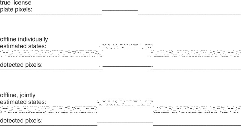
Figure 5.15 Offline state estimation

Figure 5.16 Detected licence plate pixels using offline estimation. (a) Individually estimated states. (b) Jointly estimated states.
5.3.3.3 Matlab® Functions for HMM
The Matlab® functions for the analysis of hidden Markov models are found in the Statistics toolbox. There are five functions:
hmmgenerate: given pt( · | · ) and pz( · | · ), generate a sequence of states and observations.hmmdecode: given pt( · | · ), pz( · | · ) and a sequence of observations, calculate the posterior probabilities of the states.hmmestimate: given a sequence of states and observations, estimate pt( · | · ) and pz( · | · ).hmmtrain: given a sequence of observations, estimate pt( · | · ) and pz( · | · ).hmmviterbi: given pt( · | · ), pz( · | · ) and a sequence of observations, calculate the most likely state sequence.
The function hmmtrain() implements the so-called Baum–Welch algorithm.
5.4 Mixed States and the Particle Filter
Sections 5.2 and 5.3 focused on special cases of the general online estimation problem. The topic of Section 5.2 was infinite discrete state estimation and in particular the linear-Gaussian case or approximations of that. Section 5.3 discussed finite discrete state estimation. We now return to the general scheme of Figure 5.2. The current section introduces the family of particle filters (PF). It is a group of estimators that try to implement the general case. These estimators use random samples to represent the probability densities, just as in the case of Parzen estimation (see Section 6.3.1). Therefore, particle filters are able to handle non-linear, non-Gaussian systems, continuous states, discrete states and even combinations. In the sequel we use probability densities (which in the discrete case must be replaced by probability functions).
5.4.1 Importance Sampling
A Monte Carlo simulation uses a set of random samples generated from a known distribution to estimate the expectation of any function of that distribution. More specifically, let x(k), k = 1, …, K be samples drawn from a conditional probability density p(x|z). Then the expectation of any function g(x) can be estimated by

Under mild conditions, the right-hand side asymptotically approximates the expectation as K increases. For instance, the conditional expectation and covariance matrix are found by substitution of g(x) = x and ![]() , respect-ively.
, respect-ively.
In the particle filter, the set x(k) depends on the time index i. It represents the posterior density p(x(i)|Z(i)). The samples are called the particles. The density can be estimated from the particles by some kernel-based method, for instance, the Parzen estimator discussed in Section 6.3.1.
A problem in the particle filter is that we do not know the posterior density beforehand. The solution is to get the samples from some other density, say q(x), called the proposal density. The various members of the PF family differ (among other things) in their choice of this density. The expectation of g(x) w.r.t. p(x|z) becomes

where
The factor 1/p(z) is a normalizing constant. It can be eliminated as follows:
Using Equations (5.40) and (5.41) we can estimate E[g(x)|z] by means of a set of samples drawn from q(x):

Being the ratio of two estimates, E[g(x)|z] is a biased estimate. However, under mild conditions, E[g(x)|z] is asymptotically unbiased and consistent as K increases. One of the requirements is that q(x) overlaps the support of p(x).
Usually, the shorter notation for the unnormalized importance weights w(k) = w(x(k)) is used. The so-called normalized importance weights are ![]() . Using that, expression (5.42) simplifies to
. Using that, expression (5.42) simplifies to

5.4.2 Resampling by Selection
Importance sampling provides us with samples x(k) and weights w(k)norm. Taken together, they represent the density p(x|z). However, we can transform this representation to a new set of samples with equal weights. The procedure to do that is selection. The purpose is to delete samples with low weights and to retain multiple copies of samples with high weights. The number of samples does not change by this; K is kept constant. The various members from the PF family may differ in the way they select the samples. However, an often used method is to draw the samples with replacement according to a multinomial distribution with probabilities w(k)norm.
Such a procedure is easily accomplished by calculation of the cumulative weights:

We generate K random numbers r(k) with k = 1, …, K. These numbers must be uniformly distributed between 0 and 1. Then, the kth sample x(k)selected in the new set is a copy of the jth sample x(j), where j is the smallest integer for which w(j)cum ≥ r(k).
Figure 5.17 is an illustration. The figure shows a density p(x) and a proposal density q(x). Samples x(k) from q(x) can represent p(x) if they are provided with weights w(k)norm∝p(x(k))/q(x(k)). These weights are visualized in Figure 5.17(d) by the radii of the circles. Resampling by selection gives an unweighted representation of p(x). In Figure 5.17(e), multiple copies of one sample are depicted as a pile. The height of the pile stands for the multiplicity of the copy.

Figure 5.17 Representation of a probability density. (a) A density p(x). (b) The proposal density q(x). (c) The 40 samples of q(x). (d) Importance sampling of p(x) using the 40 samples of q(x). (e) Selected samples from (d) as an equally weighted sample representation of p(x).
5.4.3 The Condensation Algorithm
One of the simplest applications of importance sampling combined with resampling by selection is in the so-called condensation algorithm (‘conditional density optimization’). The algorithm follows the general scheme of Figure 5.2. The prediction density p(x(i)|Z(i − 1)) is used as the proposal density q(x). Therefore, at time i, we assume that a set x(k) is available that is an unweighted representation of p(x(i)|Z(i − 1)). We use importance sampling to find the posterior density p(x(i)|Z(i)). For that purpose we make the following substitutions in Equation (5.40):

The weights w(k)norm that define the representation of p(x(i)|z(i)) are obtained from
Next, resampling by selection provides an unweighted representation x(k)selected. The last step is the prediction. Using x(k)selected as a representation for p(x(i)|Z(i)), the representation of p(x(i + 1)|Z(i)) is found by generating one new sample x(k) for each sample x(k)selected using p(x(i + 1)|x(k)selected) as the density to draw from. The algorithm is as follows.
Algorithm 5.4 The condensation algorithm
- Initialization:
- Set i = 0
- Draw K samples x(k), k = 1, …, K, from the prior probability density p(x(0))
- Update using importance sampling:
- Set the importance weights equal to w(k) = p(z(i)|x(k))
- Calculate the normalized importance weights:

- Resample by selection:
- Calculate the cumulative weights

- For k = 1, …, K:
- Generate a random number r uniformly distributed in [0, 1]
- Find the smallest j such that w(j)cum ≥ r(k)
- Set x(k)selected = x(j)
- Calculate the cumulative weights
- Predict:
- Set i = i + 1
- For k = 1, …, K:
- Draw sample x(k) from the density p(x(i)|x(i − 1) = x(k)selected)
- Go to 2.
After step 2, the posterior density is available in terms of the samples x(k) and the weights w(k)norm. The MMSE estimate and the associated error covariance matrix can be obtained from Equation (5.43). For instance, the MMSE is obtained by the substitution of g(x) = x. Since we have a representation of the posterior density, estimates associated with other criteria can be obtained as well.
The calculation of the importance weights in step 2 involves the conditional density p(z(i)|x(k)). In the case of the non-linear measurement functions of the type z(i) = h(x(i)) + v(i), all that remains is to calculate the density of the measurement noise for v(i) = z(i) − h(x(k)). For instance, if v(i) is zero mean, Gaussian with covariance matrix Cv, the weights are calculated as
The actual value of constant is irrelevant because of the normalization.
The drawing of new samples in the prediction step involves the state equation. If x(i + 1) = f(x(i), u(i)) + w(i), then the drawing is governed by the density of w(i).
The advantages of the particle filtering are obvious. Non-linearities of both the state equation and the measurement function are handled smoothly without the necessity to calculate Jacobian matrices. However, the method works well only if enough particles are used. Especially for large dimensions of the state vector the required number becomes large. If the number is not sufficient, then the particles are not able to represent the density p(x(i)|Z(i − 1)). In particular, if for some values of x(i) the likelihood p(z(i)|x(i)) is very large while on these locations p(x(i)|Z(i − 1)) is small, the particle filtering may not converge. If this occurs frequently then all weights become zero except one, which becomes unity. The particle filter is said to be degenerated.
Example 5.10 Particle filtering applied to volume density estimation The problem of estimating the volume density of a substance mixed with a liquid is introduced in Example 5.2. The model, expressed in Equation (5.5), is non-linear and non-Gaussian. The state vector consists of two continuous variables (volume and density) and one discrete variable (the state of the on/off controller). The measurement system, expressed in Equation (5.27), is non-linear with additive Gaussian noise. Example 5.6 has shown that the EKF is able to estimate the density, but only by using an approximate model of the process in which the discrete state is removed. The price to pay for such a rough approximation is that the estimation error of the density and (particularly) the volume has a large magnitude.
The particle filter does not need such a rough approximation because it can handle the discrete state variable. In addition, the particle filter can cope with discontinuities. These discontinuities appear here because of the discrete on/off control and also because the input flow of the substance occurs in chunks at some random points in time.
The particle filter implemented in this example uses the process model given in (5.9), and the measurement model of (5.27). The parameters used are tabulated in Example 5.5. Other parameters are: Vlow = 3990 (litres) and Vhigh = 4010 (litres). The random points of the substance are modelled as a Poisson process with mean time between two points λ = 100Δ = 100(s). The chunks have a uniform distribution between 7 and 13 (litres). Results of the particle filter using 10000 particles are shown in Figure 5.18. The figure shows an example of a cloud of particles. Clearly, such a cloud is not represented by a Gaussian distribution. In fact, the distribution is multimodal due to the uncertainty of the moment at which the on/off control switches its state.
In contrast with the Kalman filter, the particle filter is able to estimate the fluctuations of the volume. In addition, the estimation of the density is much more accurate. The price to pay is the computational cost.


Figure 5.18 Application of particle filtering to the density estimation problem. (a) Real states and measurements. (b) The particles obtained at i = 511. (c) Results.
5.4.3.1 Matlab® Functions for Particle Filtering
Many Matlab® users have already implemented particle filters, but no formal toolbox yet exists. Section 9.4 contains a listing of Matlab® code that implements the condensation algorithm. Details of the implementation are also given.
5.5 Genetic State Estimation
Genetic algorithms (GAs) simulate the processes of evolution of biological systems. They are knowledge-based information systems using the principles of evolution, natural selection and genetics to offer a method for a parallel search of complex spaces. Genetic algorithms have a huge number of application areas such as automatic control, production scheduling, data mining, image processing, etc. Basically, a GA is an optimization process using techniques that are based on Mendel's genetic inheritance concept and Darwin's theory of evolution and survival of the fittest. This section introduces an approach that uses a genetic algorithm to estimate the plant parameters and hence to obtain the state estimation James et al. (2000).
5.5.1 The Genetic Algorithm
In order for the GA to find the optimal solution to a particular problem, the parameters that comprise a solution must be encoded into a form upon which the GA can operate. Borrowing terms from biology and genetics, any set of parameters that may be a solution to the given problem is called a chromosome and the individual parameters in a chromosome are called traits. Each trait is encoded with a finite number of digits, called genes. The entire set of chromosomes upon which the GA will operate is called a population.
The assignment of the individual genes is important. The classic GA is usually a base-2 GA, in which all traits are encoded as binary numbers and all genes may take a value of 0 or 1. However, this is not necessary. In fact, a particular gene can take any one of a given number of values, called alleles. For example, a base-10 GA can be used in which each gene can take any value from 0 to 9 and, in addition, an extra gene representing the sign ± may be required for each trait. Compared to base-2 GAs, a base-10 GA has a simpler encoding and decoding procedure, and thus offers easier monitoring of the dynamics of the operation of the GA. In a real-time system simplification of the encode and decode procedure is especially important since they must occur within the sampling interval.
The GAs use the genetic operators to simulate the evolution process in order to find the best solution candidate. The genetic operators, including selection, crossover and mutation, are used to manipulate the chromosomes in a population so as to seek a chromosome that maximizes some user-defined objective function, which is called the fitness function. The GAs perform the operation iteratively. Each iteration, consisting of four steps illustrated further below, generates a new combination of the chromosomes called next generation. At the final iteration, the fittest member of the current generation, which is in fact the member with the highest fitness value, is taken to be the solution of the GA optimization problem.
The transition from one generation to the next generation consists of the following basic steps.
The first step is selection. This is a mechanism for selecting individuals for reproduction according to their fitness. To create two new chromosomes (or children), two chromosomes must be selected from the current generation as parents. As is seen in nature, those members of the population most likely to have a chance at reproducing are the members that are the fittest. There are a number of different techniques for selection in literature. A popular selection method is that the chromosomes of the population corresponding to the fittest members are automatically selected for reproducing. Therefore, those chromosomes with the least fitness have no chance of contributing any genetic material to the next generation. From the fittest members of the current population, parents are randomly chosen with equal probability.
Once two parents have been selected, the crossover operation is used. Mimicking inheritance in natural genetics, this is a method of merging the genetic information of two individuals. It causes the exchange of genetic material between the parent chromosomes, resulting in two new chromosomes. Given the two parent chromosomes, crossover occurs with a user-defined probability pc. If crossover occurs exactly once for every trait, then pc should be set as pc = 1. When crossover occurs for a trait, a randomly chosen ‘cross site’ within that trait is determined. All genes between the cross site and the end of the trait are exchanged between the parent chromosomes. Crossover helps to seek for other solutions near to solutions that appear to be good.
After the new generation has been created, each new member is subjected to mutation. In real evolution, the genetic material can by changed randomly by erroneous reproduction or other deformations of genes, for example by gamma radiation. In genetic algorithms, mutation occurs on a gene-by-gene basis. It can be realized as a random deformation of the traits with a certain probability pm. The gene that is to mutate will be replaced by a randomly chosen allele. The positive effect of mutation is the preservation of genetic diversity and, as an effect, so that a local solution to the optimization problem can be avoided. The reason is that if all of the members of a population should happen to converge to some local optimum, the mutation operator allows the possibility that a chromosome could be pulled away from that local optimum, improving the chances of finding the global optimum. However, pm should be chosen carefully. A high mutation rate results in a random walk through the GA search space, which indicates that pm should be chosen to be somewhat small; nevertheless in some instances in real-time systems, a slightly higher mutation rate is needed. If the fitness function depends on the dynamically changing state of a system, the locality of an optimum is time-dependent and we must ensure that the GA is readily capable of exploring new opportunities for maximizing the time-varying fitness functions.
An additional operator known as elitism can be applied, which causes the single fittest chromosome of a population to survive, undisturbed, in the next generation. The motivation behind elitism is that after some sufficiently small amount of time, a candidate solution may be found to be close to the optimal solution. To allow manipulation of this candidate solution would risk unsatisfactory performance by the GA. Therefore, with elitism, the fitness of the best member of the population should be a non-decreasing function from one generation to the next. If elitism is selected, the fittest member of the current generation is automatically chosen to be a member of the next generation. The remaining members are generated by selection, crossover and mutation. Many times elitism can involve more than just one member, that is a certain number ρD of the fittest members will survive in the next generation without manipulation by crossover or mutation. If the fittest member would point to a local optimum in the GA search space but a slightly less fit member points to the global optimum, they might both survive in the next generation with this new form of elitism.
The final step is sampling. This is the procedure that computes a new generation from the previous one and its offspring. Also, if a chromosome is generated by crossover and mutation, it is possible that one or more of its traits will lie outside the allowable range(s). If this occurs, each trait that is out of range should be replaced with a randomly selected trait that does fall within the allowable range.
To initialize the GA, the population size N, the allowable range for each trait and a chromosome length must be specified, along with the length and position of each trait on a chromosome. The method of generating the first population also needs to be determined. The individual members may be initialized to some set of ‘best guesses’ or, more typically, they may be randomly generated. In addition, the probabilities pc and pm discussed above must be specified. After this initialization, the GA can operate freely to solve the optimization problem.
5.5.2 Genetic State Estimation
Consider a system reformulated from Equations (5.1) and (5.8):
where ![]() is a time-invariant vector representing the system parameters. The GA-based parameter estimator assumes that the structures of f and h in (5.44) are known. The estimator can be represented as
is a time-invariant vector representing the system parameters. The GA-based parameter estimator assumes that the structures of f and h in (5.44) are known. The estimator can be represented as

where ![]() is the estimate of
is the estimate of ![]() at time i,
at time i, ![]() is the state of this estimated system and
is the state of this estimated system and ![]() is the measurement of the estimated system.
is the measurement of the estimated system.
The GA's operation on Equation (5.45) is shown by the block diagram in Figure 5.19. Each parameter estimate in the vector ![]() is encoded by the GA as a trait on a chromosome. Therefore, each chromosome completely represents a set of parameter estimates
is encoded by the GA as a trait on a chromosome. Therefore, each chromosome completely represents a set of parameter estimates ![]() , and hence it completely represents an estimated system because the structures of f and h are assumed to be known. Since the GA works with a population of chromosomes, the block in Figure 5.19 representing the estimated system can be thought of as a population of candidate systems. The GA employs the selection, crossover, mutation and elitism operators on this population of candidate systems to evolve a system that best represents the true system. At any time i, the current set of parameter estimates
, and hence it completely represents an estimated system because the structures of f and h are assumed to be known. Since the GA works with a population of chromosomes, the block in Figure 5.19 representing the estimated system can be thought of as a population of candidate systems. The GA employs the selection, crossover, mutation and elitism operators on this population of candidate systems to evolve a system that best represents the true system. At any time i, the current set of parameter estimates ![]() will be provided by the fittest chromosome in the population at time i.
will be provided by the fittest chromosome in the population at time i.

Figure 5.19 A general GA-based state estimator.
There are many different choices of fitness functions representing different strategies. As an illustration we suppose that the fitness function for the GA is chosen to minimize the squared error between the output z(i) of the actual system and that of the estimated system ![]() over a window of the l + 1 most recent data points. Therefore the fitness function takes the form
over a window of the l + 1 most recent data points. Therefore the fitness function takes the form
where

with ![]() for i > 0 and ei = 0 for i ≤ 0. To guarantee that each member has a positive fitness value, α is selected to be the highest value of (ETE)/2 of any member of the population at time i.
for i > 0 and ei = 0 for i ≤ 0. To guarantee that each member has a positive fitness value, α is selected to be the highest value of (ETE)/2 of any member of the population at time i.
Each iteration, the GA uses the current population of parameter estimates, along with the past and present values of the input u(i) and measurement z(i), to generate past and present estimated system states ![]() . A window of
. A window of ![]() values,
values, ![]() , is generated for each candidate set of parameter estimates, specifying an ‘identifier model’. Each candidate is assigned a fitness value according to the fitness function given in Equations (5.46) and (5.47). The GA selects the candidates with the highest fitness values as parents for generating the next generation of candidate sets of parameter estimates.
, is generated for each candidate set of parameter estimates, specifying an ‘identifier model’. Each candidate is assigned a fitness value according to the fitness function given in Equations (5.46) and (5.47). The GA selects the candidates with the highest fitness values as parents for generating the next generation of candidate sets of parameter estimates.
5.5.3 Computational Issues
In order to assess the possibility of implementing the genetic state estimator in real-time, computational complexity must be examined. There are two factors contributing to this issue, which are the fitness calculation procedure and the generation of the next population of chromosomes. For any given generation, let na, nm, ri and rf represent the number of additions, the numbers of multiplications, random integer generations and random floating-point number generations that must take place, respectively. The values for na and nm are of primary interest in determining the complexity of the fitness calculation procedure, while ri and rf are of primary interest in terms of generating the next population of chromosomes.
For the fitness calculation, let us consider the ℓ + 1 most recent data points. Each chromosome must undergo ℓ + 1 additions for a calculation of the error between the actual system measurement and the estimated system measurement for the data points. Then, ℓ + 1 multiplications need to be carried out for calculation of the squared error. All of the squared errors over the data window need to be added together, resulting in another ℓ additions. Therefore a total of 2ℓ + 1 additions and ℓ + 2 multiplications are needed for each chromosome in the population to generate (ETE)/2.
After the calculations of (ETE)/2 for individual chromosomes, if α is determined, N additions are needed to perform the remainder calculations of J = α − (ETE)/2 for the whole population, where N is the size of the population. Therefore, the total calculation work load can be summarized as
Depending on the encoding and decoding procedures used for chromosome manipulation, these numbers may require adjustment.
Random number generations take place in the operations of selection, crossover and mutation. First, let us check the process of selection. After the pool of the best D chromosomes is determined, every two children are generated by two parents randomly chosen from the pool. Thus each child can be thought of as the result of one random selection from the pool of D possible parents. Since we have ρD chromosomes survive in the next population by elitism, N − ρD random integer generations are needed due to parent selection. Second, we check the process of crossover. For every two children generated, nt crossover operations will occur, where nt is the number of traits on a chromosome. This means that (nt/2)(N − ρD) random integer generations will occur due to crossover operations. Finally, if ng is used to denote the number of genes per chromosome, then the number of mutation operations taking place in a given population can range from zero to ng(N − ρD), with an average value of pmng(N − ρD), where pm is the probability of mutation defined earlier. Therefore, ri, the number of random integer generations needed to produce a new population, lies in the range
with an average value
As discussed in Section 5.5.1, it is possible that mutation or crossover will lead to traits that lie outside the allowable ranges. The GA may be required to replace faulty traits with new, randomly generated traits. This will result in extra generation of random floating-point numbers. Recalling that rf denotes the number of random floating-point number generations, it can be seen that rf is in the following range:
Example 5.11 A jet engine compressor This example, presented by James et al. (2000), shows a jet engine compressor implemented through a genetic state estimator.
To achieve maximum performance from the engines used on current aircraft, those engines must often be operated near the boundaries of instability (i.e. with reduced stall and surge margins, and hence reduced safety margins). As a result, problems such as surge and rotating stall may develop when a heavy demand is placed on an aircraft engine. Surge can be described as a large-amplitude oscillation in the mass flow through the engine, sometimes resulting in a momentary reverse in flow. When surge occurs, an aircraft may experience a phenomenon known as ‘flameout’. Rotating stall consists of one or more localized regions or cells of reduced mass flow that will rotate around the circumference of the engine compressor. A rotating stall cell can grow in magnitude and, if it does so, it will grow in a circumferential manner. Clearly, problems such as surge and rotating stall are hazardous and avoidance of these problems is always desired.
The non-linear model for surge and rotating stall is expressed in a three-state form in Krstic and Kokotovic (1995). This three-state model is written as

where ΦJ is the mass flow, ΨJ is the pressure rise, RJ ≥ 0 is the normalized stall cell squared amplitude, ΦT is the mass flow through the throttle and σ, β and ΨC0 are constant parameters (with σ > 0 and β > 0). For the purpose of simulation, the values of the parameters have been chosen to be ΨC0 = 0.5, σ = 7 and 1/β2 = 0.4823. To generate the control input ΦT(i), a proportional-integral (PI) controller was used, taking as its input the error between ΨJ(i)† and a reference signal, which is represented by the dash–dot lines in Figure 5.20. The PI controller parameters used were Kp = 5 and Ki = 2. Note that the controller was implemented in discrete time.
It would be useful if some method for detecting the existence of surge and rotating stall. Surge would be evident in an oscillation of the state ΦJ, which represents the mass flow, and rotating stall activity would be evident in the behaviour of the state RJ. The ability to detect the onset of either problem would result in the execution of measures that could help prevent system failure. Unfortunately, neither of the states ΦJ and RJ is measurable during aircraft operation. The only measurable state is ΨJ, so some method for estimating ΦJ and RJ from the available information (i.e. ΨJ and ΦT) is desired.
Since the system is neither linear nor in observer form, the GA can be used for estimating ΦJ and RJ. The compressor model of Equation (5.125) must first be approximated in discrete time, so using a forward-looking difference the model can be written as

The GA actively estimates parameters of the jet engine compressor model and uses these parameter estimates along with ΨJ and ΦT to generate the estimates ![]() and
and ![]() . For this purpose, the equations used by the GA are
. For this purpose, the equations used by the GA are

where the estimates for ΨC0 + 1 have been combined to form the single-parameter estimate ![]() .
.

Figure 5.20 GA-based state estimation for the jet engine compressor model, ΨJ(0) = 0.5, RJ(0) = 0.1 and ΦJ(0) = 0.8. Plot 1 corresponds to ΨJ, plot 2 corresponds to ΦJ and plot 3 corresponds to RJ. The dotted lines in the right two plots indicate the actual state, while the solid lines indicate the state estimates. The dash–dot line in plot 1 indicates the reference input for ΨJ (adopted from James et al., 2000).
The fitness function for the GA takes the same windowed data approach found in Equation (5.46), with ![]() for i > 0 and ei = 0 for i ≤ 0. Again, note that since this fitness function is primarily focused upon driving the error between ΨJ(i) and
for i > 0 and ei = 0 for i ≤ 0. Again, note that since this fitness function is primarily focused upon driving the error between ΨJ(i) and ![]() to zero, there is no guarantee that the state estimates
to zero, there is no guarantee that the state estimates ![]() and
and ![]() will accurately track the true states ΦJ(i) and RJ(i), respectively. However, due to the dependence of each state on the other two states, it again seems at least possible that acceptable state tracking will occur.
will accurately track the true states ΦJ(i) and RJ(i), respectively. However, due to the dependence of each state on the other two states, it again seems at least possible that acceptable state tracking will occur.
Initial conditions ΨJ(0) = 0.5, RJ(0) = 0.1 and ΦJ(0) = 0.8 are used. Also, the following GA parameters are used, after some tuning: N = 200, pm = 0.2, D = 66, ρD = 8, ℓ = 100 and gt = 10. The ranges for ![]() ,
, ![]() ,
, ![]() ,
, ![]() ,
, ![]() and
and ![]() were [1.0, 2.0], [1.2, 1.8], [0.2, 0.8], [2.0, 4.0], [0.3, 0.7] and [5.0, 9.0], respectively. The initial state estimates are chosen to be
were [1.0, 2.0], [1.2, 1.8], [0.2, 0.8], [2.0, 4.0], [0.3, 0.7] and [5.0, 9.0], respectively. The initial state estimates are chosen to be ![]() and
and ![]() because a stable equilibrium point of the jet engine compressor model occurs when ΦJ(0) = 1.0 and because choosing
because a stable equilibrium point of the jet engine compressor model occurs when ΦJ(0) = 1.0 and because choosing ![]() would result in
would result in ![]() for all i ≥ 0. The results are shown in Figure 5.20, which was adopted from James et al. (2000).
for all i ≥ 0. The results are shown in Figure 5.20, which was adopted from James et al. (2000).
The GA-based state estimator for the jet engine compressor model was simulated for 25 s with T = 0.01. To verify the validity of the results, 50 simulations were executed and squared error sums were generated for ![]() and
and ![]() . The results are given in Table 5.1 presented by James et al. (2000). The squared error sums for the simulations shown in Figure 5.20 are given in the tables to verify that the figures correspond to average or typical GA simulations.
. The results are given in Table 5.1 presented by James et al. (2000). The squared error sums for the simulations shown in Figure 5.20 are given in the tables to verify that the figures correspond to average or typical GA simulations.
Table 5.1 Squared error sums for GA-based state estimation of the jet engine compressor model (adopted from James et al., 2000)
| Average | 186.77 | 226.11 |
| Minimum | 45.29 | 47.53 |
| Maximum | 697.34 | 602.34 |
| Shown in Figure 5.20 | 144.81 | 275.74 |
Source: Gremling 2000. Reproduced with permission of Elsevier.
From the figures it can be seen that the GA performed quite well. It shows that the GA is a useful tool for gaining information about non-measurable states in non-linear systems.
5.6 State Estimation in Practice
The previous sections discussed the theory needed for the design of a state estimator. This section addresses the practical issues related to the design. Usually the engineer cycles through a number of design stages of which some are depicted in Figure 5.21.
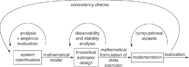
Figure 5.21 Design stages for state estimators.
One of the first steps in the design process is system identification. The purpose is to formulate a mathematical model of the system of interest. As stated in Section 5.1, the model is composed of two parts: the state space model of the physical process and the measurement model of the sensory system. Using these models, the theory from previous sections provides us with the mathematical expressions of the optimal estimator.
The next questions in the design process are the issues of observability (can all states of the process be estimated from the given set of measurements?) and stability. If the system is not observable or not stable, either the model must be revised or the sensory system must be redesigned.
If the design passes the observability and the stability tests, attention is focused on the computational issues. Due to finite arithmetic precision, there might be some pitfalls. Since in a state estimation the measurements are processed sequentially, the effects of round-off errors may accumulate and may cause inaccurate results. The estimator may even completely fail to work due to numerical instabilities. Although the optimal solution of an estimation problem is often unique, there are a number of different implementations that are all mathematically equivalent, and thus all representing the same solution but with different sensitivities to round-off errors. Thus, in this stage of the design process the appropriate implementation must be selected.
As soon as the estimator has been realized, consistency checks must be performed to see whether the estimator behaves in accordance with the expectations. If these checks fail, it is necessary to return to an earlier stage, that is refinements of the models, selection of another implementation, etc.
This section addresses the practical issues including:
- A short introduction to system identification. The topic is a discipline on its own and will certainly not be covered here in its full length. For a full treatment we refer to the pertinent literature (Box and Jenkins, 1976; Eykhoff, 1974; Ljung and Glad, 1994; Ljung, 1999; Söderström and Stoica, 1989).
- The observability and the dynamic stability of an estimator.
- The computational issues. Here, several implementations are given each with its own sensitivities to numerical instabilities.
- Consistency checks.
Some aspects of state estimator design are not discussed in this book, for instance sensitivity analysis and error budgets (see Gelb et al., 1974). These techniques are systemic methods for the identification of the most vulnerable parts of the design.
Most topics in this section concern Kalman filtering as introduced in Section 5.2.1, though some are also of relevance for extended Kalman filtering. The point of departure in Kalman filtering is a linear-Gaussian model of the physical process (Equations (5.13) and (5.20)). The MMSE solution to the online estimation problem is developed in Section 5.2.1 and is known as the discrete Kalman filter. The solution is an iterative scheme. Each iteration cycles through Equations (5.22) and (5.23).
5.6.1 System Identification
System identification is the act of formulating a mathematical model of a given dynamic system based on input and output measurements of that system and on general knowledge of the physical process at hand. The discipline of system identification not only finds application in estimator design but also in monitoring, fault detection and diagnosis (e.g. for maintenance of machines) and design of control systems.
A dichotomy of models exists between parametric models and non-parametric models. The non-parametric models describe the system by means of tabulated data of, for instance, the Fourier transfer function(s) or the edge response(s). Various types of parametric models exist, for example state space models, poles–zeros models and so on. In our case, state space models are the most useful, but other parametric models can also be used since most of these models can be converted to a state space model.
The identification process can roughly be broken down into four parts: structuring, experiment design, estimation, evaluation and selection.
5.6.1.1 Structuring
The structure of the model is settled by addressing the following questions. What is considered part of the system and what is environment? What are the (controllable) input variables? What are the possible disturbances (process noise)? What are the state variables? What are the output variables? What are the physical laws that relate to the physical variables? Which parameters of these laws are known and which are unknown? Which of these parameters can be measured directly?
Usually, there is not a unique answer to all these questions. In fact, the result of structuring is a set of candidate models.
5.6.1.2 Experiment Design
The purpose of the experimentation is to enable the determination of the unknown parameters and the evaluation and selection of the candidate models. The experiment comes down to the enforcement of some input test signals to the system at hand and the acquisition of measured data. The design aspects of the experiments are the choice of input signals, the choice of the sensors and the sensor locations and the pre-processing of the data.
The input signals should be such that the relevant aspects of the system at hand are sufficiently covered. The bandwidth of the input signal must match the bandwidth of interest. The signal magnitude must be in a range as required by the application. Furthermore, the signal energy should be sufficiently large so as to achieve suitable signal-to-noise ratios at the output of the sensors. Here, a trade-off exists between the bandwidth, the registration interval and the signal magnitude.
For instance, a very short input pulse covers a large bandwidth and permits a low registration interval, but requires a tremendous (perhaps excessive) magnitude in order to have sufficient signal-to-noise ratios. At the other side of the extremes, a single sinusoidal burst with a long duration covers only a very narrow bandwidth, and the signal magnitude can be kept low yet offering enough signal energy. A signal often used is the pseudo-random binary signal.
The choice of sensors is another issue. First, the set of identifiable, unknown parameters of the model must be determined. Sometimes it might be necessary to temporarily use additional (often expensive) sensors so as to enable the estimation of all relevant parameters. As soon as the system identification is satisfactorily accomplished, these additional sensors can be removed from the system.
In order to prevent overfitting, it might be useful to split the data according to two time intervals. The data in the first interval are used for parameter estimation. The second interval is used for model evaluation. Cross-evaluation might also be useful.
5.6.1.3 Parameter Estimation
Suppose that all unknown parameters are gathered in one parameter vector α. The discrete system equation is denoted by f(x, w, α). The measurement system is modelled, as before, by z = h(x, v). We then have the sequence of measurements according to the following recursions:

where I is the length of the sequence, x(0) is the initial condition (which may be known or unknown) and v(i) and w(i) are the measurement noise and the process noise, respectively.
One possibility for estimating α is to process the sequence z(i) in batches. For that purpose, we stack all measurement vectors to one I × n (recall that n is the dimension of z(i)) dimensional vector Z. Equation (5.49) defines the conditional probability density p(Z|α). The stochastic nature of Z is due to the randomness of w(i), v(i) and possibly x(0). Equation (5.49) shows how this randomness propagates to Z. Once the conditional density p(Z|α) has been settled, the complete estimation machinery from Chapter 4 applies, thus providing the optimal solution of α. Especially, maximum likelihood estimation is popular since (5.49) can be used to calculate the (log-) likelihood of α. A numerical optimization procedure must provide the solution.
Working in batches soon becomes complicated due to the (often) non-linear nature of the relations involved in Equation (5.49). Many alternative techniques have been developed. For linear systems, processing in the frequency domain may be advantageous. Another possibility is to process the measurements sequentially. The trick is to regard the parameters as state vectors α(i). Static parameters do not change in time. Therefore, the corresponding state equation is α(i + 1) = α(i). Sometimes, it is useful to allow slow variations in α(i). This is helpful in order to model drift phenomena, but also to improve the convergence properties of the procedure. A simple model would be a process that is similar to a random walk: α(i + 1) = α(i) + ω(i). The white noise sequence ω(i) is the driving force for the changes. Its covariance matrix Cω should be small in order to prevent a too wild behaviour of α(i).
Using this model, Equation (5.49) is transformed into:

The original state vector ![]() has been augmented with α(i). The new state equation can be written as ξ(i + 1) = ϕ(ξ(i), w(i), ω(i)) with
has been augmented with α(i). The new state equation can be written as ξ(i + 1) = ϕ(ξ(i), w(i), ω(i)) with ![]() . This opens the door to simultaneous online estimation of both x(i) and α(i) using the techniques discussed earlier in this chapter. However, the new state function ϕ( · ) is non-linear and for online estimation we must resort to estimators that can handle these non-linearities, for example extended Kalman filtering (Section 5.2.2) or particle filtering (Section 5.4).
. This opens the door to simultaneous online estimation of both x(i) and α(i) using the techniques discussed earlier in this chapter. However, the new state function ϕ( · ) is non-linear and for online estimation we must resort to estimators that can handle these non-linearities, for example extended Kalman filtering (Section 5.2.2) or particle filtering (Section 5.4).
Note that if ω(i) ≡ 0, then α(i) is a random constant and (hopefully) its estimate ![]() converges to a constant. If we allow ω(i) to deviate from zero by setting Cω to some (small) non-zero diagonal matrix, the estimator becomes adaptive. It has the potential to keep track of parameters that drift.
converges to a constant. If we allow ω(i) to deviate from zero by setting Cω to some (small) non-zero diagonal matrix, the estimator becomes adaptive. It has the potential to keep track of parameters that drift.
5.6.1.4 Evaluation and Model Selection
The last step is the evaluation of the candidate models and the final selection. For that purpose, we select a quality measure and evaluate and compare the various models. Popular quality measures are the log-likelihood and the sum of squares of the residuals (the difference between measurements and model-predicted measurements).
Models with a low order are preferable because the risk of overfitting is minimized and the estimators are less sensitive to estimation errors of the parameters. Therefore, it might be beneficial to consider not only the model with the best quality measure but also the models that score slightly less, but with a lower order. In order to evaluate these models, other tests are useful. Ideally, the cross correlation between the residuals and the input signal is zero. If not, there is still part of the behaviour of the system that is not explained by the model.
5.6.2 Observability, Controllability and Stability
5.6.2.1 Observability
We consider a deterministic linear system, which is a special case of Equations (5.13) and (5.20):

The system is called observable if with known F(i), L(i)u(i) and H(i) the state x(i) (with fixed i) can be solved from a sequence z(i), z(i + 1), … of measurements. The system is called completely observable if it is observable for any i. It can be assumed that L(i)u(i) = 0. This is without any loss of generality since the influence to z(i), z(i + 1), … of an L(i)u(i) not being zero can be neutralized easily. Hence, the observability of a system solely depends on F(i) and H(i).
An approach to find out whether the system is observable is to construct the observability Gramian (Bar-Shalom and Li, 1993). From Equation (5.50):

Equation (5.51) is of the type z = H. The least squares estimate is ![]() (see Section 4.3.1). The solution exists if and only if the inverse of HTH exists, or in other words, if the rank of HTH is equal to the dimension m of the state vector. Equivalent conditions are that HTH is positive definite (i.e. yTHTHy > 0 for every y ≠ 0) or that the eigenvalues of HTH are all positive (see Appendix B.5).
(see Section 4.3.1). The solution exists if and only if the inverse of HTH exists, or in other words, if the rank of HTH is equal to the dimension m of the state vector. Equivalent conditions are that HTH is positive definite (i.e. yTHTHy > 0 for every y ≠ 0) or that the eigenvalues of HTH are all positive (see Appendix B.5).
Translated to the present case, the requirement is that for at least one K ≥ 0 the observability Gramian ![]() , defined by
, defined by

has rank equal to m. Equivalently we check whether the Gramian is positive definite. For time-invariant systems, F and H do not depend on time and the Gramian simplifies to

If the system F is stable (the magnitude of all eigenvalues of F are less than one), we can set K → ∞ to check whether the system is observable.
A second approach to determine the observability of a time-invariant, deterministic system is to construct the observability matrix:

According to Equation (5.51), x(i) can be retrieved from a sequence z(i), …, z(i + m − 1) if ![]() is invertible; that is if the rank of
is invertible; that is if the rank of ![]() equals m.
equals m.
The advantage of using the observability Gramian instead of the observability matrix is that the former is more stable. Modelling errors and round-off errors in the coefficients in both F and H could make the difference between an invertible ![]() or
or ![]() and a non-invertible one. However,
and a non-invertible one. However, ![]() is less prone to small errors than
is less prone to small errors than ![]() .
.
A more quantitative measure of the observability is obtained by using the eigenvalues of the Gramian ![]() . A suitable measure is the ratio between the smallest eigenvalue and the largest eigenvalue. The system is less observable as this ratio tends to zero. A likewise result can be obtained by using the singular values of the matrix
. A suitable measure is the ratio between the smallest eigenvalue and the largest eigenvalue. The system is less observable as this ratio tends to zero. A likewise result can be obtained by using the singular values of the matrix ![]() (see singular value decomposition in Appendix B.6).
(see singular value decomposition in Appendix B.6).
5.6.2.2 Controllability
In control theory, the concept of controllability usually refers to the ability that for any state x(i) at a given time i a finite input sequence u(i), u(i + 1), …, u(i + ℓ − 1) exists that can drive the system to an arbitrary final state x(i + ℓ). If this is possible for any time, the system is called completely controllable. As with observability, the controllability of a system can be revealed by checking the rank of a Gramian. For time-invariant systems, the controllability can also be analysed by means of the controllability matrix. This matrix arises from the following equation:

The minimum number of steps, ℓ, is at most equal to m, the dimension of the state vector. Therefore, in order to test the controllability of the system (F, L) it suffices to check whether the controllability matrix (L FL … Fm − 1L) has rank m.
The Matlab® functions for creating the controllability matrix and Gramian are ctrb() and gram(), respectively.
5.6.2.3 Dynamic Stability and Steady State Solutions
The term stability refers to the ability of a system to resist to and recover from disturbances acting on this system. A state estimator has to face three different causes of instabilities: sensor instability, numerical instability, and dynamic instability.
Apart from the usual sensor noise and sensor linearity errors, a sensor may produce unusual glitches and other errors caused by phenomena hard to predict, such as radio interference, magnetic interference, thermal drift, mechanical shocks, and so on. This kind of behaviour is sometimes denoted by sensor instability. Its early detection can be done using consistency checks (to be discussed later in this section).
Numerical instabilities originate from round-off errors. Particularly, the inversion of a near singular matrix may cause large errors due to its sensitivity to round-off errors. A careful implementation of the design must prevent these errors (see Section 5.6.3).
The third cause for instability lies in the dynamics of the state estimator itself. In order to study the dynamic stability of the state estimator it is necessary to consider the estimator as a dynamic system with as inputs the measurements z(i) and the control vectors u(i) (see Appendix D). The output consists of the estimates ![]() . In linear systems, the stability does not depend on the input sequences. For the stability analysis it suffices to assume zero z(i) and u(i). The equations of interest are derived from (5.22) and (5.23):
. In linear systems, the stability does not depend on the input sequences. For the stability analysis it suffices to assume zero z(i) and u(i). The equations of interest are derived from (5.22) and (5.23):
with
where P(i) is the covariance matrix C(i + 1|i) of the predicted state ![]() and P(i) is recursively defined by the discrete Ricatti equation:
and P(i) is recursively defined by the discrete Ricatti equation:

The recursion starts with ![]() . The first term in Equation (5.53) represents the absorption of uncertainty due to the dynamics of the system during each time step (provided that F is stable; otherwise it represents the growth of uncertainty). The second term represents the additional uncertainty at each time step due to the process noise. The last term represents the reduction of uncertainty thanks to the measurements.
. The first term in Equation (5.53) represents the absorption of uncertainty due to the dynamics of the system during each time step (provided that F is stable; otherwise it represents the growth of uncertainty). The second term represents the additional uncertainty at each time step due to the process noise. The last term represents the reduction of uncertainty thanks to the measurements.
For the stability analysis of a Kalman filter it is of interest to know whether a sequence of process noise, w(i), can influence each element of the state vector independently. The answer to this question is found by writing the covariance matrix Cw(i) of the process noise as Cw(i) = G(i)GT(i). Here, G(i) can be obtained by an eigenvalue/eigenvector diagonalization of Cw(i), that is Cw(i) = Vw(i)Λw(i)VTw(i) and G(i) = Vw(i)Λ1/2w(i) (see Appendix B.5 and C.3). Λw(i) is a K × K diagonal matrix where K is the number of nonzero eigenvalues of Cw(i). The matrices G(i) and Vw(i) are K × K matrices. The introduction of G(i) allows us to write the system equation as:
where ![]() is a K-dimensional Gaussian white noise vector with covariance matrix I. The noise sequence w(i) influences each element of x(i) independently if the system (F(i), G(i)) is controllable by the sequence
is a K-dimensional Gaussian white noise vector with covariance matrix I. The noise sequence w(i) influences each element of x(i) independently if the system (F(i), G(i)) is controllable by the sequence ![]() . We then have the following theorem (Bar-Shalom and Li, 1993), which provides a sufficient (but not a necessary) condition for stability:
. We then have the following theorem (Bar-Shalom and Li, 1993), which provides a sufficient (but not a necessary) condition for stability:
If a time-invariant system (F, H) is completely observable and the system (F, G) is completely controllable, then for any initial condition P(0) = Cx(0) the solution of the Ricatti equation converges to a unique, finite, invertible steady state covariance matrix P(∞).
The observability of the system ensures that the sequence of measurements contains information about the complete state vector. Therefore, the observability guarantees that the prediction covariance matrix P(∞) is bounded from above. Consequently, the steady state Kalman filter is BIBO stable (see Appendix D.3.2). If one or more state elements are not observable, the Kalman gains for these elements will be zero and the estimation of these elements is purely prediction driven (model based without using measurements). If the system F is unstable for these elements, then so is the Kalman filter.
The controllability with respect to ![]() ensures that P(∞) is unique (does not depend on Cx(0)) and that its inverse exists. If the system is not controllable, then P(∞) might depend on the specific choice of Cx(0). If for the non-controllable state elements the system F is stable, then the corresponding eigenvalues of P(∞) are zero. Consequently, the Kalman gains for these elements are zero and the estimation of these elements is again purely prediction driven.
ensures that P(∞) is unique (does not depend on Cx(0)) and that its inverse exists. If the system is not controllable, then P(∞) might depend on the specific choice of Cx(0). If for the non-controllable state elements the system F is stable, then the corresponding eigenvalues of P(∞) are zero. Consequently, the Kalman gains for these elements are zero and the estimation of these elements is again purely prediction driven.
The discrete algebraic Ricatti equation, P(i + 1) = P(i), mentioned earlier in this chapter, provides the steady state solution for the Ricatti equation:
The steady state is reached due to the balance between the growth of uncertainty (the second term and possibly the first term) and the reduction of uncertainty (the third term and possibly the first term).
A steady state solution of the Ricatti equation gives rise to a constant Kalman gain. The corresponding Kalman filter, derived from Equations (5.22), (5.23) and (5.52),
with
becomes time invariant.
5.6.3 Computational Issues
A straightforward implementation of the time-variant Kalman filter may result in too large estimation errors. The magnitudes of these errors are not compatible with the error covariance matrices. The filter may even completely diverge even though theoretically the filter should be stable. This anomalous behaviour is due to a number representation with limited precisions. In order to find where round-off errors have the largest impact it is instructive to rephrase the Kalman equations in (5.22) and (5.23) as follows:
Ricatti loop:

Estimation loop:

For simplicity, the system (F, L, H) is written without the time index.
As can be seen, the filter consists of two loops. If the Kalman filter is stable, the second loop (the estimation loop) is usually not that sensitive to round-off errors. Possible induced errors are filtered in much the same way as the measurement noise. However, the loop depends on the Kalman gains K(i). Large errors in K(i) may cause the filter to become unstable. These gains come from the first loop.
In the first loop (the Ricatti loop) the prediction covariance matrix P(i) = C(i + 1|i) is recursively calculated. As can be seen, the recursion involves non-linear matrix operations including a matrix inversion. Especially, the representation of these matrices (and through this the Kalman gain) may be sensitive to the effects of round-off errors.
The sensitivity to round-off errors becomes apparent if an eigenvalue–eigenvector decomposition (Appendix B.5 and C.3.2) is applied to the covariance matrix P:

where λk are the eigenvalues of P and vk the corresponding eigenvectors. The eigenvalues of a properly behaving covariance matrix are all positive (the matrix is positive definite and non-singular). However, the range of the eigenvalues may be very large. This finds expression in the condition number λmax/λmin of the matrix. Here, λmax = max(λk) and λmin = min(λk). A large condition number indicates that if the matrix is inverted, the propagation of round-off errors will be large:

In a floating-point representation of P, the exponents are largely determined by λmax. Therefore, the round-off error in λmin is proportional to λmax and may be severe. It will result in large errors in 1/λmin.
Another operation with a large sensitivity to round-off errors is the subtraction of two similar matrices.
These errors can result in a loss of symmetry in the covariance matrices and a loss of positive definiteness. In some cases, the eigenvalues of the covariance matrices can even become negative. If this occurs, the errors may accumulate during each recursion and the process may diverge.
As an example, consider the following Ricatti loop:

This loop is mathematically equivalent to Equations (5.22) and (5.23), but is computationally less expensive because the factor HC(i|i − 1) appears at several places and can be reused. However, the form is prone to round-off errors because:
- The part K(i)H can easily introduce asymmetries in C(i|i).
- The subtraction I − K(i)H can introduce negative eigenvalues.
The implementation should be used cautiously. The preferred implementation is Equation (5.22):
It requires more operations than expression (5.54) but it is more balanced. Therefore, the risk of introducing asymmetries is much lower. Still, this implementation does not guarantee non-negative eigenvalues.
Listing 5.2 implements the Kalman filter using Equation (5.55). The functions acquire_measurement_vector() and get_control_vector() are place holders for the interfacing to the measurement system and a possible control system. These functions should also take care of the timing of the estimation process. The required number of operations (using Matlab®'s standard matrix arithmetic) of the update step is about 2m2n + 3mn2 + n3. The number of the operations of the prediction step is about 2m3.
Listing 5.2 Conventional time-variant Kalman filter for a time-invariant system
prload linsys;       % Load a system: F,H,Cw,Cv,Cx0,x0,L
C=Cx0;                % Initialize prior uncertainty
xprediction=x0;      % and prior mean
while (1)            % Endless loop
  % Update:
  S=H*C*H'+Cv;       % Innovation matrix
  K=C*H'*S^-1;        % Kalman gain matrix
  z =acquire_measurement_vector();
  innovation =z - H*xprediction;
  xestimation = xprediction+K*innovation;
  C=C - K*S*K';
  % Prediction:
  u=get_control_vector();
  xprediction=F*xestimation+L*u;
  C=F*C*F'+Cw;
end
The symmetry of a matrix P can be enforced by the assignment: P: =(P + PT)/2. The addition of this type of statement at some critical locations in the code helps a little, but often not enough. The true remedy is to use a proper implementation combined with sufficient number precision.
5.6.4 Consistency Checks
We now provide some tools that enable the designer to check whether his design behaves consistently (Bar-Shalom and Birmiwal, 1983). As discussed in the previous sections, the two main reasons why a realized filter does not behave correctly are modelling errors and numerical instabilities of the filter.
Estimators are related with three types of error variances:
- The minimal variances that would be obtained with the most appropriate model.
- The actual variances of the estimation errors of some given estimator.
- The variances indicated by the calculated error covariance matrix of a given estimator.
Of course, the purpose is to find an estimator whose error variances equal the first one. Since we do not know whether our model approaches the most appropriate one, we do not have the guarantee that our design approaches the minimal attainable variance. However, if we have reached the optimal solution, then the actual variances of the estimation errors must coincide with the calculated variances. Such a correspondence between actual and calculated variances is a necessary condition for an optimal filter, but not a sufficient one.
Unfortunately, we need to know the real estimation errors in order to check whether the two variances coincide. This is only possible if the physical process is (temporarily) provided with additional instruments that give us reference values of the states. Usually such provisions are costly, so we focus the discussion on the checks that can be accomplished without reference values.
5.6.4.1 Orthogonality Properties
We recall that in linear-Gaussian systems, the innovations (residuals) vectors ![]() in the update step of the Kalman filter (5.22) are zero mean with the innovation matrix as covariance matrix:
in the update step of the Kalman filter (5.22) are zero mean with the innovation matrix as covariance matrix:
Furthermore, let ![]() be the estimation error of the estimate
be the estimation error of the estimate ![]() . We then have the following properties:
. We then have the following properties:

These properties follow from the principle of orthogonality. In the static case, any unbiased linear MMSE satisfies
The last step follows from K = CxzC− 1z (see Equation (4.29)). The principle of orthogonality, ![]() , simply states that the covariance between any component of the error and any measurement is zero. Adopting an inner product definition for two random variables ek and zl as
, simply states that the covariance between any component of the error and any measurement is zero. Adopting an inner product definition for two random variables ek and zl as ![]() , the principle can be expressed as e ⊥ z.
, the principle can be expressed as e ⊥ z.
Since x(i|j) is an unbiased linear MMSE estimate, it is a linear function of the set ![]() . According to the principle of orthogonality, we have e(i|j) ⊥ Z(j). Therefore, e(i|j) must also be orthogonal to any z(l), where l ≤ j, because z(l) is a subspace of Z(j). This proves the first statement in Equation (5.56).
. According to the principle of orthogonality, we have e(i|j) ⊥ Z(j). Therefore, e(i|j) must also be orthogonal to any z(l), where l ≤ j, because z(l) is a subspace of Z(j). This proves the first statement in Equation (5.56).
In addition, x(k|l), l ≤ j, is a linear combination of Z(l). Therefore, it is also orthogonal to e(i|j), which proves the second statement.
The whiteness property of the innovations follows from the following argument. Suppose j < i. We may write ![]() . In the inner expectation, the measurements Z(j) are known. Since
. In the inner expectation, the measurements Z(j) are known. Since ![]() is a linear combination of Z(j),
is a linear combination of Z(j), ![]() is non-random. It can be taken outside the inner expectation:
is non-random. It can be taken outside the inner expectation: ![]() . However,
. However, ![]() must be zero because the predicted measurements are unbiased estimates of the true measurements. If
must be zero because the predicted measurements are unbiased estimates of the true measurements. If ![]() , then
, then ![]() (unless i = j).
(unless i = j).
5.6.4.2 Normalized Errors
The NEES (normalized estimation error squared) is a test signal defined as
In the linear-Gaussian case, the NEES has a χ2m distribution (chi-square with m degrees of freedom; see Appendix C.1.5).
The χ2m distribution of the NEES follows from the following argument. Since the state estimator is unbiased, E[e(i|i)] = 0. The covariance matrix of e(i|i) is C(i|i). Suppose A(i) is a symmetric matrix such that A(i)AT(i) = C− 1(i|i). Application of A(i) to e(i) will give a random vector y(i) = A(i)e(i). The covariance matrix of y(i) is A(i)C(i|i)AT(i) = A(i)(A(i)AT(i))− 1AT(i) = I. Thus, the components of y(i) are uncorrelated and have unit variance. If both the process noise and the measurement noise are normally distributed, then so is y(i). Hence, the inner product yT(i)y(i) = eT(i)C− 1(i|i)e(i) is the sum of m squared, independent random variables, each normally distributed with zero mean and unit variance. Such a sum has a χ2m distribution.
The NIS (normalized innovation squared) is a test signal defined as
In the linear-Gaussian case, the NIS has a χ2n distribution. This follows readily from the same argument as used above.
5.6.4.3 Consistency Checks
From Equation (5.56) and the properties of the NEES and the NIS, the following statement holds true.
If a state estimator for a linear-Gaussian system is optimal, then:
- The sequence Nees(i) must be χ2m distributed.
- The sequence Nis(i) must be χ2n distributed.
- The sequence
 (innovations) must be white.
Consistency checks of a ‘state estimator-under-test’ can be performed by collecting the three sequences and by applying statistical tests to see whether the three conditions are fulfilled. If one or more of these conditions are not satisfied, then we may conclude that the estimator is not optimal.
In a real design, the NEES test is only possible if the true states are known. As mentioned above, such is the case when the system is (temporarily) provided with extra measurement equipment that measures the states directly and with sufficient accuracy so that their outputs can be used as a reference. Usually such measurement devices are too expensive and the designer has to rely on the other two tests. However, the NEES test is applicable in simulations of the physical process. It can be used to see if the design is very sensitive to changes in the parameters of the model. The other two tests use the innovations. Since the innovations are always available, even in a real design, these are of more practical significance.
In order to check the hypothesis that a dataset obeys a given distribution, we have to apply a distribution test. Examples are the Kolmogorov–Smirnov test and the chi-square test (Section 9.4.3). Often, instead of these rigorous tests a quick procedure suffices to give an indication. We simply determine an interval in which, say, 95% of the samples must be. Such an interval [A, B] is defined by F(B) − F(A) = 0.95. Here, F( · ) is the probability distribution of the random variable under test. If an appreciable part of the dataset is outside this interval, then the hypothesis is rejected. For chi-square distributions there is the one-sided 95% acceptance boundary with A = 0 and B such that ![]() . Sometimes the two-sided 95% acceptance boundaries are used, defined by
. Sometimes the two-sided 95% acceptance boundaries are used, defined by ![]() and
and ![]() . Table 5.2 gives values of A and B for various degrees of freedom (Dof).
. Table 5.2 gives values of A and B for various degrees of freedom (Dof).
Table 5.2 Acceptance boundaries of 95% for χ2Dof distributions
| One-sided | Two-sided | |||
| Dof | A | B | A | B |
| 1 | 0 | 3.841 | 0.0010 | 5.024 |
| 2 | 0 | 5.991 | 0.0506 | 7.378 |
| 3 | 0 | 7.815 | 0.2158 | 9.348 |
| 4 | 0 | 9.488 | 0.4844 | 11.14 |
| 5 | 0 | 11.07 | 0.8312 | 12.83 |
For state estimators that have reached the steady state, S(i) is constant and the whiteness property of the innovations implies that the power spectrum of any element of ![]() must be flat. Suppose that
must be flat. Suppose that ![]() is an element of
is an element of ![]() . The variance of
. The variance of ![]() , denoted by σ2l, is the lth diagonal element in S. The discrete Fourier transform of
, denoted by σ2l, is the lth diagonal element in S. The discrete Fourier transform of ![]() , calculated over i = 0, …, I − 1, is
, calculated over i = 0, …, I − 1, is

The periodogram of ![]() , defined here as
, defined here as ![]() , is an estimate of the power spectrum (Blackman and Tukey, 1958). If the power spectrum is flat, then E[Pl(k)] = σ2l. It can be proven that in that case the variables 2Pl(k)/σ2l is χ22 distributed for all k (except for k = 0). Hence, the whiteness of
, is an estimate of the power spectrum (Blackman and Tukey, 1958). If the power spectrum is flat, then E[Pl(k)] = σ2l. It can be proven that in that case the variables 2Pl(k)/σ2l is χ22 distributed for all k (except for k = 0). Hence, the whiteness of ![]() is tested by checking whether 2Pl(k)/σ2l is χ22 distributed.
is tested by checking whether 2Pl(k)/σ2l is χ22 distributed.
5.6.4.4 Fudging
If one or more of the consistency checks fail, then somewhere a serious modelling error has occurred. The designer has to step back to an earlier stage of the design in order to identify the fault. The problem can be caused anywhere, from inaccurate modelling during the system identification to improper implementations. If the system is non-linear and the extended Kalman filter is applied, problems may arise due to the neglect of higher-order terms of the Taylor series expansion.
A heuristic method to catch the errors that arise due to approximations of the model is to deliberately increase the modelled process noise (Bar-Shalom and Li, 1993). One way to do so is by increasing the covariance matrix Cw of the process noise by means of a fudge factor γ. For instance, we simply replace Cw by Cw + γI. Instead of adapting Cw we can also increase the diagonal of the prediction covariance C(i + 1|i) by some factor. The fudge factor should be selected such that the consistency checks now pass as successfully as possible.
Fudging causes a decrease of faith in the model of the process and thus causes a larger impact of the measurements. However, modelling errors give rise to deviations that are autocorrelated and not independent from the states. Thus, these deviations are not accurately modelled by white noise. The designer should maintain a critical attitude with respect to fudging.
5.7 Selected Bibliography
Some introductory books on Kalman filtering and its applications are Anderson and Moore (1979), Bar-Shalom and Li (1993), Gelb et al. (1974) and Grewal and Andrews (2001). Hidden Markov models are described in Rabiner (1989). Tutorials on particle filtering are found in Arulampalam et al. (2002) and Merwe et al. (2000). These tutorials also describe some shortcomings of the particle filter and possible remedies. Seminal papers for Kalman filtering, particle filtering and unscented Kalman filtering are Kalman (1960), Gordon et al. (1993) and Julier and Uhlmann (1997), respectively. Linear systems with random inputs, among which are the AR models, are studied in Box and Jenkins (1976). The topic of statistical linearization is treated in Gelb et al. (1974). The condensation algorithm is due to Isard and Blake (1996). The Baum-Welch algorithm is described in Rabiner (1986). Excellent explanation and examples of GA based state estimation can be found in James et al. (2000).
- Anderson, B.D. and Moore, J.B., Optimal Filtering, Prentice Hall, Englewood Cliffs, NJ, 1979.
 mström, K.J. and Wittenmark, B., Computer-Controlled Systems – Theory and Design, Second Edition, Prentice Hall, Englewood Cliffs, NJ, 1990.
- Arulampalam, M.S., Maskell, S., Gordon, N. and Clapp, T., A tutorial on particle filters for online nonlinear/non-Gaussian Bayesian tracking, IEEE Transactions on Signal Processing, 50(2), 174–188, February 2002.
- Bar-Shalom, Y. and Birmiwal, K., Consistency and robustness of PDAF for target tracking in cluttered environments, Automatica, 19, 431–437, July 1983.
- Bar-Shalom, Y. and Li, X.R., Estimation and Tracking – Principles, Techniques, and Software, Artech House, Boston, MA, 1993.
- Blackman, R.B. and Tukey, J.W., The Measurement of Power Spectra, Dover, New York, 1958.
- Box, G.E.P. and Jenkins, G.M., Time Series Analysis: Forecasting and Control, Holden-Day, San Francisco, CA, 1976.
- Bryson, A.E. and Hendrikson, L.J., Estimation using sampled data containing sequentially correlated noise, Journal of Spacecraft and Rockets, 5(6), 662–665, June 1968.
- Eykhoff, P., System Identification, Parameter and State Estimation, John Wiley & Sons, Ltd, London, 1974.
- Gelb, A., Kasper, J.F., Nash, R.A., Price, C.F. and Sutherland, A.A., Applied Optimal Estimation, MIT Press, Cambridge, MA, 1974.
- Gordon, N.J., Salmond, D.J. and Smith, A.F.M., Novel approach to nonlinear/nonGaussian Bayesian state estimation, IEE Proceedings-F, 140(2), 107–113, 1993.
- Grewal, M.S. and Andrews, A.P., Kalman Filtering – Theory and Practice Using Matlab, Second Edition, John Wiley & Sons, Inc., New York, 2001.
- Isard, M. and Blake, A., Contour tracking by stochastic propagation of conditional density, European Conference on Computer Vision, pp. 343–56, Cambridge, UK, 1996.
- James, R., Gremling, K. and Passino, M., Genetic adaptive state estimation, Engineering Applications of Artificial Intelligence, 13 (2000), 611–623.
- Julier, S.J. and Uhlmann, J.K., A new extension of the Kalman filter to nonlinear systems, Proceedings of AeroSense: the 11th International Symposium on Aerospace/Defence Sensing, Simulation and Controls, Vol. Multi Sensor, Tracking and Resource Management II, Orlando, Florida, 1997.
- Kalman, R.E., A new approach to linear filtering and prediction problems, ASME Journal of Basic Engineering, 82, 34–45, 1960.
- Kaminski, P.G., Bryson, A.E. and Schmidt, J.F., Discrete square root filtering: a survey of current techniques, IEEE Transactions on Automatic Control, 16 (6), 727–736, December 1971.
- Krstic, M. and Kokotovic, P.V., Lean backstepping design for a jet engine compressor model. IEEE Conference on Control Applications, 1995.
- van der Merwe, R., Doucet, A., de Freitas, N. and Wan, E. The unscented particle filter, Technical report CUED/F-INFENG/TR 380, Cambridge University Engineering Department, 2000.
- Ljung, L., System Identification – Theory for the User, Second Edition, Prentice Hall, Upper Saddle River, NJ, 1999.
- Ljung, L. and Glad, T., Modeling of Dynamic Systems, Prentice Hall, Englewood Cliffs, NJ, 1994.
- Potter, J.E. and Stern, R.G., Statistical filtering of space navigation measurements, Proceedings of AIAA Guidance and Control Conference, AIAA, New York, 1963.
- Rabiner, L.R., A tutorial on hidden Markov models and selected applications in speech recognition, Proceedings of the IEEE, 77 (2), 257–285, February 1989.
- Rauch, H.E., Tung, F. and Striebel, C.T., Maximum likelihood estimates of linear dynamic systems, AIAA Journal, 3 (8), 1445–1450, August 1965.
- Söderström, T. and Stoica, P., System Identification, Prentice Hall International, London, 1989.
Exercises
-
Consider the following model for a random constant:

The prior knowledge is E[x(0)] = 0 and σ2x(0) = ∞. Give the expression for the solution of the discrete Lyapunov equation.
-
For the random constant model given in Exercise 1, give expressions for the innovation matrix S(i), the Kalman gain matrix K(i), the error covariance matrix C(i|i) and the prediction matrix C(i|i − 1) for the first few time steps, that is for i = 0, 1, 2 and 3. Explain the results.
-
In Exercise 2, can you find the expressions for arbitrary i. Can you also prove that these expressions are correct? Hint: use induction. Explain the results.
-
Consider the following time-invariant scalar linear-Gaussian system:

The prior knowledge is Ex(0) = 0 and σ2x(0) = ∞. What is the condition for the existence of the solution of the discrete Lyapunov equation? If this condition is met, give an expression for that solution.
-
For the system described in Exercise 4, give the steady state solution, that is, give expressions for S(i), K(i), C(i|i) and C(i|i − 1) if i → ∞.
-
For the system given in Exercise 4, give expressions for S(i), K(i), C(i|i) and C(i|i − 1) for the first few time steps, that is, i = 0, 1, 2 and 3. Explain the results.
-
In Exercise 4, can you find the expressions for S(i), K(i), C(i|i) and C(i|i − 1) for arbitrary i?
-
Autoregressive models and Matlab®'s Control System Toolbox: consider the following second-order autoregressive (AR) model:

Using the functions
tf()andss()from the Control Toolbox, convert this AR model into an equivalent state space model, that is, x(i + 1) = Fx(i) + Gw(i) and z(i) = Hx(i) + v(i). (Usehelp tfandhelp ssto find out how these functions should be used.) Assuming that w(i) and v(i) are white noise sequences with variances σ2w = 1 and σ2v = 1, use the functiondlyap()to find the solution of the discrete Lyapunov equation and the functionkalman()(ordlqe()) to find the solution for the steady state Kalman gain and corresponding error covariance matrices. Hint: the output variable of the commandss()is a ‘struct’ whose fields are printed by typingstruct(ss). -
Moving average models: repeat Exercise 8, but now considering the so-called first order moving average (MA) model:

-
Autoregressive, moving average models: repeat Exercise 8, but now considering the so-called ARMA(2, 1) model:

-
Simulate the processes mentioned in Exercises 1, 8, 9 and 10, using Matlab®, and apply the Kalman filters.