
4
Parameter Estimation
Parameter estimation is the process of attributing a parametric description to an object, a physical process or an event based on measurements that are obtained from that object (or process, or event). The measurements are made available by a sensory system. Figure 4.1 gives an overview. Parameter estimation and pattern classification are similar processes because they both aim to describe an object using measurements. However, in parameter estimation the description is in terms of a real-valued scalar or vector, whereas in classification the description is in terms of just one class selected from a finite number of classes.

Figure 4.1 Parameter estimation.
Example 4.1 Estimation of the backscattering coefficient from SAR images In Earth observations based on airborne SAR (synthetic aperture radar) imaging, the physical parameter of interest is the backscattering coefficient. This parameter provides information about the condition of the surface of the Earth, e.g. soil type, moisture content, crop type, growth of the crop.
The mean backscattered energy of a radar signal in a direction is proportional to this backscattering coefficient. In order to reduce so-called speckle noise the given direction is probed a number of times. The results are averaged to yield the final measurement. Figure 4.2 shows a large number of realizations of the true backscattering coefficient and its corresponding measurement.1 In this example, the number of probes per measurement is eight. It can be seen that, even after averaging, the measurement is still inaccurate. Moreover, although the true backscattering coefficient is always between 0 and 1, the measurements can easily violate this constraint (some measurements are greater than 1).
The task of a parameter estimator here is to map each measurement to an estimate of the corresponding backscattering coefficient.

Figure 4.2 Different realizations of the backscattering coefficient and its corresponding measurement.
This chapter addresses the problem of how to design a parameter estimator. For that, two approaches exist: Bayesian estimation (Section 4.1) and data-fitting techniques (Section 4.3). The Bayesian-theoretic framework for parameter estimation follows the same line of reasoning as the one for classification (as discussed in Chapter 3). It is a probabilistic approach. The second approach, data fitting, does not have such a probabilistic context. The various criteria for the evaluation of an estimator are discussed in Section 4.2.
4.1 Bayesian Estimation
Figure 4.3 gives a framework in which parameter estimation can be defined. The starting point is a probabilistic experiment where the outcome is a random vector x defined in ℝM and with probability density p(x). Associated with x is a physical object, process or event (in short, ‘physical object’), of which x is a property; x is called a parameter vector and its density p(x) is called the prior probability density.

Figure 4.3 Parameter estimation.
The object is sensed by a sensory system that produces an N-dimensional measurement vector z. The task of the parameter estimator is to recover the original parameter vector x given the measurement vector z. This is done by means of the estimation function ![]() . The conditional probability density p(z|x) gives the connection between the parameter vector and measurements. With fixed x, the randomness of the measurement vector z is due to physical noise sources in the sensor system and other unpredictable phenomena. The randomness is characterized by p(z|x). The overall probability density of z is found by averaging the conditional density over the complete parameter space:
. The conditional probability density p(z|x) gives the connection between the parameter vector and measurements. With fixed x, the randomness of the measurement vector z is due to physical noise sources in the sensor system and other unpredictable phenomena. The randomness is characterized by p(z|x). The overall probability density of z is found by averaging the conditional density over the complete parameter space:
The integral extends over the entire M-dimensional space ℝM.
Finally, Bayes’ theorem for conditional probabilities gives us the posterior probability density p(x|z):
This density is most useful since z, being the output of the sensory system, is at our disposal and thus fully known. Thus, p(x|z) represents exactly the knowledge that we have on x after having observed z.
Example 4.2 Estimation of the backscattering coefficient The backscattering coefficient x from Example 4.1 is within the interval [0, 1]. In most applications, however, lower values of the coefficient occur more frequently than higher ones. Such a preference can be taken into account by means of the prior probability density p(x). We will assume that for a certain application x has a beta distribution:
The parameters a and b are the shape parameters of the distribution. In Figure 4.4(a) these parameters are set to a = 1 and b = 4. These values will be used throughout the examples in this chapter. Note that there is no physical evidence for the beta distribution of x. The assumption is a subjective result of our state of knowledge concerning the occurrence of x. If no such knowledge is available, a uniform distribution between 0 and 1 (i.e. all x are equally likely) would be more reasonable.
The measurement is denoted by z. The mathematical model for SAR measurements is that, with fixed x, the variable Nprobesz/x has a gamma distribution with parameter Nprobes (the number of probes per measurement). The probability density associated with a gamma distribution is
where u is the independent variable, Γ(α) is the gamma function, a is the parameter of the distribution and U(u) is the unit step function, which returns 0 if u is negative and 1 otherwise. Since z can be regarded as a gamma-distributed random variable scaled by a factor x/Nprobes, the conditional density of z becomes

Figure 4.4(b) shows the conditional density.

Figure 4.4 Probability densities for the backscattering coefficient. (a) Prior density p(x). (b) Conditional density p(z|x) with Nprobes = 8. The two axes have been scaled with x and 1/x, respectively, to obtain invariance with respect to x.
Cost Functions
The optimization criterion of Bayes, minimum risk, applies to statistical parameter estimation provided that two conditions are met. First, it must be possible to quantify the cost involved when the estimates differ from the true parameters. Second, the expectation of the cost, the risk, should be acceptable as an optimization criterion.
Suppose that the damage is quantified by a cost function ![]() . Ideally, this function represents the true cost. In most applications, however, it is difficult to quantify the cost accurately. Therefore, it is common practice to choose a cost function whose mathematical treatment is not too complex. Often, the assumption is that the cost function only depends on the difference between estimated and true parameters: the estimation error
. Ideally, this function represents the true cost. In most applications, however, it is difficult to quantify the cost accurately. Therefore, it is common practice to choose a cost function whose mathematical treatment is not too complex. Often, the assumption is that the cost function only depends on the difference between estimated and true parameters: the estimation error ![]() . With this assumption, the following cost functions are well known (see Table 4.1):
. With this assumption, the following cost functions are well known (see Table 4.1):
Table 4.1 Three different Bayesian estimators worked out for the scalar case.
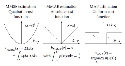
- Quadratic cost function:
(4.6)
- Absolute value cost function:
(4.7)

- Uniform cost function:
(4.8)

The first two cost functions are instances of the Minkowski distance measures (see Appendix A.2). The third cost function is an approximation of the distance measure mentioned in Equation (A.22).
Risk Minimization
With an arbitrarily selected estimate ![]() and a given measurement vector z, the conditional risk of
and a given measurement vector z, the conditional risk of ![]() is defined as the expectation of the cost function:
is defined as the expectation of the cost function:
In Bayes’ estimation (or minimum risk estimation) the estimate is the parameter vector that minimizes the risk:
The minimization extends over the entire parameter space.
The overall risk (also called the average risk) of an estimator ![]() is the expected cost seen over the full set of possible measurements:
is the expected cost seen over the full set of possible measurements:
Minimization of the integral is accomplished by minimization of the integrand. However, since p(z) is positive, it suffices to minimize ![]() . Therefore, the Bayes estimator not only minimizes the conditional risk but also the overall risk.
. Therefore, the Bayes estimator not only minimizes the conditional risk but also the overall risk.
The Bayes solution is obtained by substituting the selected cost function in Equations (4.9) and (4.10). Differentiating and equating it to zero yields, for the three cost functions given in Equations (4.6), (4.7) and (4.8):
- MMSE estimation (MMSE = minimum mean square error).
- MMAE estimation (MMAE = minimum mean absolute error).
- MAP estimation (MAP = maximum a posterior).
Table 4.1 gives the solutions that are obtained if x is a scalar. The MMSE and the MAP estimators will be worked out for the vectorial case in the next sections. However, first the scalar case will be illustrated by means of an example.
Example 4.3 Estimation of the backscattering coefficient The estimators for the backscattering coefficient (see the previous example) take the form depicted in Figure 4.5. These estimators are found by substitution of Equations (4.3) and (4.5) in the expressions in Table 4.1.
In this example, the three estimators do not differ much. Nevertheless, their own typical behaviours manifest themselves clearly if we evaluate their results empirically. This can be done by means of the population of the Npop = 500 realisations that are shown in the figure. For each sample zi we calculate the average cost ![]() , where xi is the true value of the ith sample and
, where xi is the true value of the ith sample and ![]() is the estimator under test. Table 4.2 gives the results of that evaluation for the three different estimators and the three different cost functions.
is the estimator under test. Table 4.2 gives the results of that evaluation for the three different estimators and the three different cost functions.
Not surprisingly, in Table 4.2 the MMSE, the MMAE and the MAP estimators are optimal with respect to their own criterion, that is the quadratic, the absolute value and the uniform cost criterion, respectively. It appears that the MMSE estimator is preferable if the cost of a large error is considerably higher than that of a small error. The MAP estimator does not discriminate between small or large errors. The MMAE estimator takes its position in between.
Matlab® code for generating Figure 4.5 is given in Listing 4.1. It uses the Statistics toolbox for calculating the various probability density functions. Although the MAP solution can be found analytically, here we approximate all three solutions numerically. To avoid confusion, it is easy to create functions that calculate the various probabilities needed. Note how p(z) = ∫p(z|x)p(x)dx is approximated by a sum over a range of values of x, whereas p(x|z) is found by Bayes’ rule.

Figure 4.5 Three different Bayesian estimators.
Table 4.2 Empirical evaluation of the three different Bayesian estimators in Figure 4.5

Listing 4.1 Matlab® code for MMSE, MMSA and MAP estimation in the scalar case.
function estimates
   global N Np a b xrange;

   N = 500;                % Number of samples
   Np = 8;                 % Number of looks
   a = 2; b = 5;           % Beta distribution parameters
   x = 0.005:0.005:1;      % Interesting range of x
   z = 0.005:0.005:1.5;    % Interesting range of z
   prload scatter;         % Load set (for plotting only)
   xrange = x;
   for i = 1:length(z)
     [dummy,ind] = max(px_z(x,z(i))); x_map(i) = x(ind);
     x_mse(i) = sum(pz_x(z(i),x).*px(x).*x)
       ./.sum(pz_x(z(i),x).*px(x));
     ind = find((cumsum(px_z(x,z(i))) ./ .sum(px_z(x,z(i))))>0.5);
     x_mae(i) = x(ind(1));
   end

   figure; clf; plot(zset,xset,`.'); hold on;
   plot(z,x_map,`k-.'); plot(z,x_mse,`k- -');
   plot(z,x_mae,`k-');
   legend(`realizations',`MAP',`MSE',`MAE');
 return
 function ret = px(x)
   global a b; ret = betapdf(x,a,b);
 return
 function ret = pz_x(z,x)
   global Np; ret = (z>0).*(Np./x).*gampdf(Np*z./x,Np,1);
 return
 function ret = pz(z)
   global xrange; ret = sum(px(xrange).*pz_x(z,xrange));
 return
 function ret = px_z(x,z)
   ret = pz_x(z,x).*px(x)./pz(z);
 return
4.1.1 MMSE Estimation
The solution based on the quadratic cost function (4.6) is called the minimum mean square error estimator, also called the minimum variance estimator for reasons that will become clear in a moment. Substitution of Equations (4.6) and (4.9) in (4.10) gives
Differentiating the function between braces with respect to ![]() (see Appendix B.4) and equating this result to zero yields a system of M linear equations, the solution of which is
(see Appendix B.4) and equating this result to zero yields a system of M linear equations, the solution of which is
The conditional risk of this solution is the sum of the variances of the estimated parameters:

and hence the name ‘minimum variance estimator’.
4.1.2 MAP Estimation
If the uniform cost function is chosen, the conditional risk (4.9) becomes

The estimate that now minimizes the risk is called the maximum a posteriori (MAP) estimate:
This solution equals the mode (maximum) of the posterior probability. It can also be written entirely in terms of the prior probability densities and the conditional probabilities:
This expression is similar to the one of MAP classification (see Equation (3.12)).
4.1.3 The Gaussian Case with Linear Sensors
Suppose that the parameter vector x has a normal distribution with expectation vector E[x] = ![]() and covariance matrix Cx. In addition, suppose that the measurement vector can be expressed as a linear combination of the parameter vector corrupted by additive Gaussian noise:
and covariance matrix Cx. In addition, suppose that the measurement vector can be expressed as a linear combination of the parameter vector corrupted by additive Gaussian noise:
where v is an N-dimensional random vector with zero expectation and covariance matrix Cv, x and v are uncorrelated, and H is an N × M matrix.
The assumption that both x and v are normal implies that the conditional probability density of z is also normal. The conditional expectation vector of z equals
The conditional covariance matrix of z is Cz|x = Cv.
Under these assumptions the posterior distribution of x is normal as well. Application of Equation (4.2) yields the following expressions for the MMSE estimate and the corresponding covariance matrix:

The proof is left as an exercise for the reader (see Exercise 4). Note that ![]() , being the posterior expectation, is the MMSE estimate
, being the posterior expectation, is the MMSE estimate ![]() .
.
The posterior expectation, E[x|z], consists of two terms. The first term is linear in z. It represents the information coming from the measurement. The second term is linear in ![]() , representing the prior knowledge. To show that this interpretation is correct it is instructive to see what happens at the extreme ends: either no information from the measurement or no prior knowledge:
, representing the prior knowledge. To show that this interpretation is correct it is instructive to see what happens at the extreme ends: either no information from the measurement or no prior knowledge:
- The measurements are useless if the matrix H is virtually zero or if the noise is too large, that is C− 1v is too small. In both cases, the second term in Equation (4.20) dominates. In the limit, the estimate becomes
 with covariance matrix Cx, that is the estimate is purely based on prior knowledge.
 -
On the other hand, if the prior knowledge is weak, that is if the variances of the parameters are very large, the inverse covariance matrix C− 1x tends to zero. In the limit, the estimate becomes
(4.21)
In this solution, the prior knowledge, that is
 , is completely ruled out.
Note that the mode of a normal distribution coincides with the expectation. Therefore, in the linear-Gaussian case, MAP estimation and MMSE estimation coincide: ![]() .
.
4.1.4 Maximum Likelihood Estimation
In many practical situations the prior knowledge needed in MAP estimation is not available. In these cases, an estimator that does not depend on prior knowledge is desirable. One attempt in that direction is the method referred to as maximum likelihood estimation (ML estimation). The method is based on the observation that in MAP estimation, Equation (4.17), the peak of the first factor p(z|x) is often in an area of x in which the second factor p(x) is almost constant. This holds true especially if little prior knowledge is available. In these cases, the prior density p(x) does not affect the position of the maximum very much. Discarding the factor and maximizing the function p(z|x) solely gives the ML estimate:
Regarded as a function of x the conditional probability density is called the likelihood function; hence the name ‘maximum likelihood estimation’.
Another motivation for the ML estimator is when we change our viewpoint with respect to the nature of the parameter vector x. In the Bayesian approach x is a random vector, statistically defined by means of probability densities. In contrast, we may also regard x as a non-random vector whose value is simply unknown. This is the so-called Fisher approach. In this view, there are no probability densities associated with x. The only density in which x appears is p(z|x), but here x must be regarded as a parameter of the density of z. From all estimators discussed so far, the only estimator that can handle this deterministic point of view on x is the ML estimator.
Example 4.4 Maximum likelihood estimation of the backscattering coefficient The maximum likelihood estimator for the backscattering coefficient (see the previous examples) is found by maximizing Equation (4.5):
The estimator is depicted in Figure 4.6 together with the MAP estimator. The figure confirms the statement above that in areas of flat prior probability density the MAP estimator and the ML estimator coincide. However, the figure also reveals that the ML estimator can produce an estimate of the backscattering coefficient that is larger than one – a physical impossibility. This is the price that we have to pay for not using prior information about the physical process.

Figure 4.6 MAP estimation, ML estimation and linear MMSE estimation.
If the measurement vector z is linear in x and corrupted by additive Gaussian noise, as given in Equation (4.18), the likelihood of x is given in Equation (4.21). Thus, in that case:
A further simplification is obtained if we assume that the noise is white, that is Cv ∼ I:
The operation (HTH)–1HT is the pseudo inverse of H. Of course, its validity depends on the existence of the inverse of HTH. Usually, such is the case if the number of measurements exceeds the number of parameters, that is N > M, which is if the system is overdetermined.
4.1.5 Unbiased Linear MMSE Estimation
The estimators discussed in the previous sections exploit full statistical knowledge of the problem. Designing such an estimator is often difficult. The first problem that arises is adequate modelling of the probability densities. Such modelling requires detailed knowledge of the physical process and the sensors. Once we have the probability densities, the second problem is how to minimize the conditional risk. Analytic solutions are often hard to obtain. Numerical solutions are often burdensome.
If we constrain the expression for the estimator to some mathematical form, the problem of designing the estimator boils down to finding the suitable parameters of that form. An example is the unbiased linear MMSE estimator, with the following form:2
The matrix K and the vector a must be optimized during the design phase in order to match the behaviour of the estimator to the problem at hand. The estimator has the same optimization criterion as the MMSE estimator, that is a quadratic cost function. The constraint results in an estimator that is not as good as the (unconstrained) MMSE estimator, but it requires only knowledge of moments up to the order two, that is expectation vectors and covariance matrices.
The starting point is the overall risk expressed in Equation (4.11). Together with the quadratic cost function we have
The optimal unbiased linear MMSE estimator is found by minimizing R with respect to K and a. Hence we differentiate R with respect to a and equate the result to zero:

yielding
with ![]() and
and ![]() the expectations of x and z.
the expectations of x and z.
Substitution of a back into Equation (4.27), differentiation with respect to K and equating the result to zero (see also Appendix B.4):

yields
where Cz is the covariance matrix of z and ![]() the cross-covariance matrix between x and z.
the cross-covariance matrix between x and z.
Example 4.5 Unbiased linear MMSE estimation of the backscattering coefficient In the scalar case, the linear MMSE estimator takes the form:
where cov[x, z] is the covariance of x and z. In the backscattering problem, the required moments are difficult to obtain analytically. However, they are easily estimated from the population of the 500 realizations shown in Figure 4.6 using techniques from Chapter 5. The resulting estimator is shown in Figure 4.6. Matlab® code to plot the ML and unbiased linear MMSE estimates of the backscattering coefficient on a data set is given in Listing 4.2.
Listing 4.2 Matlab® code for an unbiased linear MMSE estimation.
 prload scatter;           % Load dataset (zset,xset)
 z = 0.005:0.005:1.5;      % Interesting range of z
 x_ml = z;                 % Maximum likelihood
 mu_x = mean(xset); mu_z = mean(zset);
 K = ((xset-mu_x)'*(zset-mu_z))*inv((zset-mu_z)'*(zset-mu_z));
 a = mu_x K*mu_z;
 x_ulmse = K*z + a;        % Unbiased linear MMSE
 figure; clf; plot(zset,xset,'.'); hold on;
 plot(z,x_ml,'k-'); plot(z,x_ulmse,'k- -');
Linear Sensors
The linear MMSE estimator takes a particular form if the sensory system is linear and the sensor noise is additive:
This case is of special interest because of its crucial role in the Kalman filter (to be discussed in Chapter 5). Suppose that the noise has zero mean with covariance matrix Cv. In addition, suppose that x and v are uncorrelated, that is Cxv = 0. Under these assumptions the moments of z are as follows:

The proof is left as an exercise for the reader.
Substitution of Equations (4.32), (4.28) and (4.29) in (4.26) gives rise to the following estimator:

This version of the unbiased linear MMSE estimator is the so-called Kalman form of the estimator.
Examination of Equation (4.20) reveals that the MMSE estimator in the Gaussian case with linear sensors is also expressed as a linear combination of ![]() and z. Thus, in this special case (that is, Gaussian densities + linear sensors)
and z. Thus, in this special case (that is, Gaussian densities + linear sensors) ![]() is a linear estimator. Since
is a linear estimator. Since ![]() and
and ![]() are based on the same optimization criterion, the two solutions must be identical here:
are based on the same optimization criterion, the two solutions must be identical here: ![]() . We conclude that Equation (4.20) is an alternative form of (4.33). The forms are mathematically equivalent (see Exercise 5).
. We conclude that Equation (4.20) is an alternative form of (4.33). The forms are mathematically equivalent (see Exercise 5).
The interpretation of ![]() is as follows. The term
is as follows. The term ![]() represents the prior knowledge. The term
represents the prior knowledge. The term ![]() is the prior knowledge that we have about the measurements. Therefore, the factor
is the prior knowledge that we have about the measurements. Therefore, the factor ![]() is the informative part of the measurements (called the innovation). The so-called Kalman gain matrix K transforms the innovation into a correction term
is the informative part of the measurements (called the innovation). The so-called Kalman gain matrix K transforms the innovation into a correction term ![]() that represents the knowledge that we have gained from the measurements.
that represents the knowledge that we have gained from the measurements.
4.2 Performance Estimators
No matter which precautions are taken, there will always be a difference between the estimate of a parameter and its true (but unknown) value. The difference is the estimation error. An estimate is useless without an indication of the magnitude of that error. Usually, such an indication is quantified in terms of the so-called bias of the estimator and the variance. The main purpose of this section is to introduce these concepts.
Suppose that the true but unknown value of a parameter is x. An estimator ![]() provides us with an estimate
provides us with an estimate ![]() based on measurements z. The estimation error e is the difference between the estimate and the true value:
based on measurements z. The estimation error e is the difference between the estimate and the true value:
Since x is unknown, e is unknown as well.
4.2.1 Bias and Covariance
The error e is composed of two parts. One part is the one that does not change value if we repeat the experiment over and over again. It is the expectation of the error, called the bias. The other part is the random part and is due to sensor noise and other random phenomena in the sensory system. Hence, we have
If x is a scalar, the variance of an estimator is the variance of e. Thus the variance quantifies the magnitude of the random part. If x is a vector, each element of e has its own variance. These variances are captured in the covariance matrix of e, which provides an economical and also a more complete way to represent the magnitude of the random error.
The application of the expectation and variance operators to e needs some discussion. Two cases must be distinguished. If x is regarded as a non-random, unknown parameter, then x is not associated with any probability density. The only randomness that enters the equations is due to the measurements z with density p(z|x). However, if x is regarded as random, it does have a probability density. We then have two sources of randomness, x and z.
We start with the first case, which applies to, for instance, the maximum likelihood estimator. Here, the bias b(x) is given by

The integral extends over the full space of z. In general, the bias depends on x. The bias of an estimator can be small or even zero in one area of x, whereas in another area the bias of that same estimator might be large.
In the second case, both x and z are random. Therefore, we define an overall bias b by taking the expectation operator now with respect to both x and z:

The integrals extend over the full space of x and z.
The overall bias must be considered as an average taken over the full range of x. To see this, rewrite p(x, z) = p(z|x)p(x) to yield
where b(x) is given in Equation (4.35).
If the overall bias of an estimator is zero, then the estimator is said to be unbiased. Suppose that in two different areas of x the biases of an estimator have opposite sign; then these two opposite biases may cancel out. We conclude that, even if an estimator is unbiased (i.e. its overall bias is zero), then this does not imply that the bias for a specific value of x is zero. Estimators that are unbiased for every x are called absolutely unbiased.
The variance of the error, which serves to quantify the random fluctuations, follows the same line of reasoning as that of the bias. First, we determine the covariance matrix of the error with non-random x:

As before, the integral extends over the full space of z. The variances of the elements of e are at the diagonal of Ce(x).
The magnitude of the full error (bias + random part) is quantified by the so-called mean square error (the second-order moment matrix of the error):

It is straightforward to prove that
This expression underlines the fact that the error is composed of a bias and a random part.
The overall mean square error Me is found by averaging Me(x) over all possible values of x:
Finally, the overall covariance matrix of the estimation error is found as

The diagonal elements of this matrix are the overall variances of the estimation errors.
The MMSE estimator and the unbiased linear MMSE estimator are always unbiased. To see this, rewrite Equation (4.36) as follows:

The inner integral is identical to zero and thus b must be zero. The proof of the unbiasedness of the unbiased linear MMSE estimator is left as an exercise.
Other properties related to the quality of an estimator are stability and robustness. In this context, stability refers to the property of being insensitive to small random errors in the measurement vector. Robustness is the property of being insensitive to large errors in a few elements of the measurements (outliers) (see Section 4.3.2). Often, the enlargement of prior knowledge increases both the stability and the robustness.
Example 4.6 Bias and variance in the backscattering application Figure 4.7 shows the bias and variance of the various estimators discussed in the previous examples. To enable a fair comparison between bias and variance in comparable units, the square root of the latter, that is the standard deviation, has been plotted. Numerical evaluation of Equations (4.37), (4.41) and (4.42) yields:3


Figure 4.7 The bias and the variance of the various estimators in the backscattering problem.
From this, and from Figure 4.7, we observe that:
- The overall bias of the ML estimator appears to be zero. Therefore, in this example, the ML estimator is unbiased (together with the two MMSE estimators, which are intrinsically unbiased). The MAP estimator is biased.
- Figure 4.7 shows that for some ranges of x the bias of the MMSE estimator is larger than its standard deviation. Nevertheless, the MMSE estimator outperforms all other estimators with respect to overall bias and variance. Hence, although a small bias is a desirable property, sometimes the overall performance of an estimator can be improved by allowing a larger bias.
- The ML estimator appears to be linear here. As such, it is comparable with the unbiased linear MMSE estimator. Of these two linear estimators, the unbiased linear MMSE estimator outperforms the ML estimator. The reason is that – unlike the ML estimator – the ulMMSE estimator exploits prior knowledge about the parameter. In addition, the ulMMSE estimator is more applicable to the evaluation criterion.
- Of the two non-linear estimators, the MMSE estimator outperforms the MAP estimator. The obvious reason is that the cost function of the MMSE estimator matches the evaluation criterion.
- Of the two MMSE estimators, the non-linear MMSE estimator outperforms the linear one. Both estimators have the same optimization criterion, but the constraint of the ulMMSE degrades its performance.
4.2.2 The Error Covariance of the Unbiased Linear MMSE Estimator
We now return to the case of having linear sensors, z = Hx + v, as discussed in Section 4.1.5. The unbiased linear MMSE estimator appeared to be (see Equation (4.33))
where Cv and Cx are the covariance matrices of v and x; ![]() is the (prior) expectation vector of x. As stated before, the
is the (prior) expectation vector of x. As stated before, the ![]() is unbiased.
is unbiased.
Due to the unbiasedness of ![]() , the mean of the estimation error
, the mean of the estimation error ![]() – x is zero. The error covariance matrix, Ce, of e expresses the uncertainty that remains after having processed the measurements. Therefore, Ce is identical to the covariance matrix associated with the posterior probability density. It is given by (Equation (4.20))
– x is zero. The error covariance matrix, Ce, of e expresses the uncertainty that remains after having processed the measurements. Therefore, Ce is identical to the covariance matrix associated with the posterior probability density. It is given by (Equation (4.20))
The inverse of a covariance matrix is called an information matrix. For instance, C− 1e is a measure of the information provided by the estimate ![]() . If the norm of C− 1e is large, then the norm of Ce must be small, implying that the uncertainty in
. If the norm of C− 1e is large, then the norm of Ce must be small, implying that the uncertainty in ![]() is small as well. Equation (4.44) shows that C− 1e is made up of two terms. The term C− 1x represents the prior information provided by
is small as well. Equation (4.44) shows that C− 1e is made up of two terms. The term C− 1x represents the prior information provided by ![]() . The matrix C− 1v represents the information that is given by z about the vector Hx. Therefore, the matrix HTC− 1vH represents the information about x provided by z. The two sources of information add up, so the information about x provided by
. The matrix C− 1v represents the information that is given by z about the vector Hx. Therefore, the matrix HTC− 1vH represents the information about x provided by z. The two sources of information add up, so the information about x provided by ![]() is C− 1e = Cx− 1 + HTC− 1vH.
is C− 1e = Cx− 1 + HTC− 1vH.
Using the matrix inversion lemma (4.10) the expression for the error covariance matrix can be given in an alternative form:
The matrix S is called the innovation matrix because it is the covariance matrix of the innovations ![]() . The factor
. The factor ![]() is a correction term for the prior expectation vector
is a correction term for the prior expectation vector ![]() . Equation (4.45) shows that the prior covariance matrix Cx is reduced by the covariance matrix KSKT of the correction term.
. Equation (4.45) shows that the prior covariance matrix Cx is reduced by the covariance matrix KSKT of the correction term.
4.3 Data Fitting
In data-fitting techniques, the measurement process is modelled as
where h(.) is the measurement function that models the sensory system and v are disturbing factors, such as sensor noise and modelling errors. The purpose of fitting is to find the parameter vector x that ‘best’ fits the measurements z.
Suppose that ![]() is an estimate of x. Such an estimate is able to ‘predict’ the modelled part of z, but it cannot predict the disturbing factors. Note that v represents both the noise and the unknown modelling errors. The prediction of the estimate
is an estimate of x. Such an estimate is able to ‘predict’ the modelled part of z, but it cannot predict the disturbing factors. Note that v represents both the noise and the unknown modelling errors. The prediction of the estimate ![]() is given by
is given by ![]() . The residuals
. The residuals ![]() are defined as the difference between observed and predicted measurements:
are defined as the difference between observed and predicted measurements:
Data fitting is the process of finding the estimate ![]() that minimizes some error norm of ‖ϵ‖, the residuals. Different error norms (see Appendix A.1.1) lead to different data fits. We will shortly discuss two error norms.
that minimizes some error norm of ‖ϵ‖, the residuals. Different error norms (see Appendix A.1.1) lead to different data fits. We will shortly discuss two error norms.
4.3.1 Least Squares Fitting
The most common error norm is the squared Euclidean norm, also called the sum of squared differences (SSD), or simply the LS norm (least squared error norm):

The least squares fit, or least squares estimate (LS), is the parameter vector that minimizes this norm:
If v is random with a normal distribution, zero mean and covariance matrix Cv = σ2vI, the LS estimate is identical to the ML estimate: ![]() . To see this, it suffices to note that in the Gaussian case the likelihood takes the form
. To see this, it suffices to note that in the Gaussian case the likelihood takes the form

The minimization of Equation (4.48) is equivalent to the minimization of Equation (4.50). If the measurement function is linear, that is z = Hx + v, and H is an N × M matrix having a rank M with M < N, then according to Equation (4.25)
Example 4.7 Repeated measurements Suppose that a scalar parameter x is N times repeatedly measured using a calibrated measurement device: zn = x + vn. These repeated measurements can be represented by a vector z = [z1, …, zN]T. The corresponding measurement matrix is H = [1, …, 1]T. Since (HTH)− 1 = 1/N, the resulting least squares fit is

In other words, the best fit is found by averaging the measurements.
Non-linear sensors
If h(.) is non-linear, an analytic solution of Equation (4.49) is often difficult. One is compelled to use a numerical solution. For that, several algorithms exist, such as ‘Gauss–Newton’, ‘Newton–Raphson’, ‘steepest descent’ and many others. Many of these algorithms are implemented within Matlab®'s optimization toolbox. The ‘Gauss–Newton’ method will be explained shortly.
Assuming that some initial estimate xref is available we expand Equation (4.46) in a Taylor series and neglect all terms of order higher than two:

where Href is the Jacobian matrix of h(.) evaluated at xref (see Appendix B.4). With such a linearization, Equation (4.51) applies. Therefore, the following approximate value of the LS estimate is obtained:
A refinement of the estimate could be achieved by repeating the procedure with the approximate value as reference. This suggests an iterative approach. Starting with some initial guess ![]() , the procedure becomes as follows:
, the procedure becomes as follows:

In each iteration, the variable i is incremented. The iterative process stops if the difference between x(i + 1) and x(i) is smaller than some predefined threshold. The success of the method depends on whether the first initial guess is already close enough to the global minimum. If not, the process will either diverge or get stuck in a local minimum.
Example 4.8 Estimation of the diameter of a blood vessel In vascular X-ray imaging, one of the interesting parameters is the diameter of blood vessels. This parameter provides information about a possible constriction. As such, it is an important aspect in cardiologic diagnosis.
Figure 4.8(a) is a (simulated) X-ray image of a blood vessel of the coronary circulation. The image quality depends on many factors. Most important are the low-pass filtered noise (called quantum mottle) and the image blurring due to the image intensifier.
Figure 4.8(b) shows the one-dimensional, vertical cross-section of the image at a location, as indicated by the two black arrows in Figure 4.8(a). Suppose that our task is to estimate the diameter of the imaged blood vessel from the given cross-section. Hence, we define a measurement vector z whose elements consist of the pixel grey values along the cross-section.
The parameter of interest is the diameter D. However, other parameters might be unknown as well, for example the position and orientation of the blood vessel, the attenuation coefficient or the intensity of the X-ray source. This example will be confined to the case where the only unknown parameters are the diameter D and the position y0 of the image blood vessel in the cross-section. Thus, the parameter vector is two-dimensional: xT = [D y0]. Since all other parameters are assumed to be known, a radiometric model can be worked out to a measurement function h(x), which quantitatively predicts the cross-section and thus also the measurement vector z for any value of the parameter vector x.

Figure 4.8 LS estimation of the diameter D and the position y0 of a blood vessel. (a) X-ray image of the blood vessel. (b) Cross-section of the image together with a fitted profile. (c) The sum of least squares errors as a function of the diameter and the position.
With this measurement function it is straightforward to calculate the LS norm ‖ϵ‖22 for a couple of values of x. Figure 4.8(c) is a graphical representation of that. It appears that the minimum of ‖ϵ‖22 is obtained if ![]() . The true diameter is D = 0.40 mm. The obtained fitted cross-section is also shown in Figure 4.8(b).
. The true diameter is D = 0.40 mm. The obtained fitted cross-section is also shown in Figure 4.8(b).
Note that the LS norm in Figure 4.8(c) is a smooth function of x. Hence, the convergence region of a numerical optimizer will be large.
4.3.2 Fitting Using a Robust Error Norm
Suppose that the measurement vector in an LS estimator has a few elements with large measurement errors, the so-called outliers. The influence of an outlier is much larger than one of the others because the LS estimator weights the errors quadratically. Consequently, the robustness of LS estimation is poor.
Much can be improved if the influence is bounded in one way or another. This is exactly the general idea of applying a robust error norm. Instead of using the sum of squared differences, the objective function of (4.48) becomes

where ρ(.) measures the size of each individual residual ![]() . This measure should be selected such that above a given level of ϵn its influence is ruled out. In addition, one would like to have ρ(.) being smooth so that numerical optimization of ‖ϵ‖robust is not too difficult. A suitable choice (among others) is the so-called Geman–McClure error norm:
. This measure should be selected such that above a given level of ϵn its influence is ruled out. In addition, one would like to have ρ(.) being smooth so that numerical optimization of ‖ϵ‖robust is not too difficult. A suitable choice (among others) is the so-called Geman–McClure error norm:
A graphical representation of this function and its derivative is shown in Figure 4.9. The parameter σ has a soft threshold value. For values of ![]() smaller than about σ, the function follows the LS norm. For values larger than σ, the function becomes saturated. Consequently, for small values of
smaller than about σ, the function follows the LS norm. For values larger than σ, the function becomes saturated. Consequently, for small values of ![]() the derivative
the derivative ![]() of ρ(.) is nearly a constant. However, for large values of
of ρ(.) is nearly a constant. However, for large values of ![]() , that is for outliers, it becomes nearly zero. Therefore, in a Gauss–Newton style of optimization, the Jacobian matrix is virtually zero for outliers. Only residuals that are about as large as σ or smaller than that play a role.
, that is for outliers, it becomes nearly zero. Therefore, in a Gauss–Newton style of optimization, the Jacobian matrix is virtually zero for outliers. Only residuals that are about as large as σ or smaller than that play a role.

Figure 4.9 A robust error norm and its derivative.
Example 4.9 Robust estimation of the diameter of a blood vessel If in Example 4.8 the diameter is estimated near the bifurcation (as indicated in Figure 4.8(a) by the white arrows) a large modelling error occurs because of the branching vessel (see the cross-section in Figure 4.10(a)). These modelling errors are large compared to the noise and they should be considered as outliers. However, Figure 4.10(b) shows that the error landscape ‖ϵ‖22 has its minimum at ![]() . The true value is D = 0.40 mm. Furthermore, the minimum is less pronounced than the one in Figure 4.8(c), and therefore also less stable.
. The true value is D = 0.40 mm. Furthermore, the minimum is less pronounced than the one in Figure 4.8(c), and therefore also less stable.
Note also that in Figure 4.10(a) the position found by the LS estimator is in the middle between the two true positions of the two vessels.
Figure 4.11 shows the improvements that were obtained by applying a robust error norm. The threshold σ is selected just above the noise level. For this setting, the error landscape clearly shows two pronounced minima corresponding to the two blood vessels. The global minimum is reached at ![]() . The estimated position now clearly corresponds to one of the two blood vessels, as shown in Figure 4.11(a).
. The estimated position now clearly corresponds to one of the two blood vessels, as shown in Figure 4.11(a).

Figure 4.10 LS estimation of the diameter D and the position y0. (a) Cross-section of the image together with a profile fitted with the LS norm. (b) The LS norm as a function of the diameter and the position.
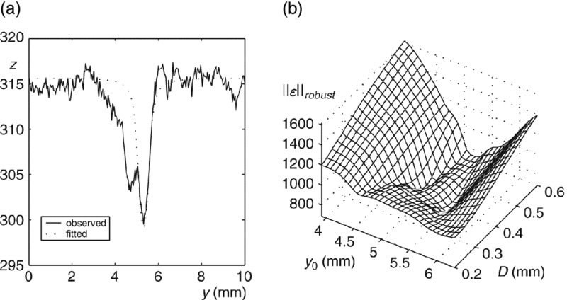
Figure 4.11 Robust estimation of the diameter D and the position y0. (a) Cross-section of the image together with a profile fitted with a robust error norm. (b) The robust error norm as a function of the diameter and the position.
4.3.3 Regression
Regression is the act of deriving an empirical function from a set of experimental data. Regression analysis considers the situation involving pairs of measurements (t, z). The variable t is regarded as a measurement without any appreciable error; t is called the independent variable. We assume that some empirical function f(.) is chosen that (hopefully) can predict z from the independent variable t. Furthermore, a parameter vector x can be used to control the behaviour of f(.). Hence, the model is
where f(.,.) is the regression curve and ϵ represents the residual, that is the part of z that cannot be predicted by f (.,.). Such a residual can originate from sensor noise (or other sources of randomness), which makes the prediction uncertain, but it can also be caused by an inadequate choice of the regression curve.
The goal of regression is to determine an estimate ![]() of the parameter vector x based on N observations (tn, zn), n = 0,…, N – 1 such that the residuals ϵn are as small as possible. We can stack the observations zn in a vector z. Using Equation (4.57), the problem of finding
of the parameter vector x based on N observations (tn, zn), n = 0,…, N – 1 such that the residuals ϵn are as small as possible. We can stack the observations zn in a vector z. Using Equation (4.57), the problem of finding ![]() can be transformed to the standard form of Equation (4.47):
can be transformed to the standard form of Equation (4.47):

where ![]() is the vector that embodies the residuals ϵn.
is the vector that embodies the residuals ϵn.
Since the model is in the standard form, x can be estimated with a least squares approach as in Section 4.3.1. Alternatively, we use a robust error norm as defined in Section 4.3.2. The minimization of such a norm is called robust regression analysis.
In the simplest case, the regression curve f(t, x) is linear in x. With that, the model takes the form ![]() , and thus the solution of Equation (4.51) applies. As an example, we consider polynomial regression for which the regression curve is a polynomial of order M – 1:
, and thus the solution of Equation (4.51) applies. As an example, we consider polynomial regression for which the regression curve is a polynomial of order M – 1:
If, for instance, M = 3, then the regression curve is a parabola described by three parameters. These parameters can be found by least squares estimation using the following model:

Example 4.10 The calibration curve of a level sensor In this example, the goal is to determine a calibration curve of a level sensor to be used in a water tank. For that purpose, a second measurement system is available with a much higher precision than the ‘sensor under test’. The measurement results of the second system serve as a reference. Figure 4.12 shows the observed errors of the sensor versus the reference values. Here, 46 pairs of measurements are shown. A zero-order (fit with a constant), a first-order (linear fit) and a tenth-order polynomial are fitted to the data. As can be seen, the constant fit appears to be inadequate for describing the data (the model is too simple). The first-order polynomial describes the data reasonably well and is also suitable for extrapolation. The tenth-order polynomial follows the measurement points better and also the noise. It cannot be used for extrapolation because it is an example of overfitting the data. This occurs whenever the model has too many degrees of freedom compared to the number of data samples.
Listing 4.3 illustrates how to fit and evaluate polynomials using Matlab®’s polyfit() and polyval() routines.

Figure 4.12 Determination of a calibration curve by means of polynomial regression.
Listing 4.3 Matlab® code for polynomial regression.
 prload levelsensor;                      % Load dataset (t,z)
 figure; clf; plot(t,z,`k.'); hold on;    % Plot it
 y = 0:0.2:30; M = [1210];plotstring = {`k- -',`k-',`k:'};
 for m = 1:3
   p = polyfit(t,z,M(m)-1);               % Fit polynomial
   z_hat = polyval(p,y);                  % Calculate plot points
   plot(y,z_hat,plotstring{m});           % and plot them
 end;
 axis([0 30 0.3 0.2]);
4.4 Overview of the Family of Estimators
The chapter concludes with the overview shown in Figure 4.13. Two main approaches have been discussed, the Bayes estimators and the fitting techniques. Both approaches are based on the minimization of an objective function. The difference is that with Bayes, the objective function is defined in the parameter domain, whereas with fitting techniques, the objective function is defined in the measurement domain. Another difference is that the Bayes approach has a probabilistic context, whereas the approach of fitting lacks such a context.

Figure 4.13 A family tree of estimators.
Within the family of Bayesian estimators we have discussed two estimators derived from two cost functions. The quadratic cost function leads to MMSE (minimum variance) estimation. The cost function is such that small errors are regarded as unimportant, while larger errors are considered more and more serious. The solution is found as the conditional mean, that is the expectation of the posterior probability density. The estimator is unbiased.
If the MMSE estimator is constrained to be linear, the solution can be expressed entirely in terms of first- and second-order moments. If, in addition, the sensory system is linear with additive, uncorrelated noise, a simple form of the estimator appears that is used in Kalman filtering. This form is sometimes referred to as the Kalman form.
The other Bayes estimator is based on the uniform cost function. This cost function is such that the damage of small and large errors are equally weighted, which leads to MAP estimation. The solution appears to be the mode of the posterior probability density. The estimator is not guaranteed to be unbiased.
It is remarkable that although the quadratic cost function and the unit cost function differ greatly, the solutions are identical provided that the posterior density is unimodal and symmetric. An example of this occurs when the prior probability density and conditional probability density are both Gaussian. In that case the posterior probability density is also Gaussian.
If no prior knowledge about the parameter is available, one can use the ML estimator. Another possibility is to resort to fitting techniques, of which the LS estimator is the most popular. The ML estimator is essentially a MAP estimator with uniform prior probability. Under the assumptions of normal distributed sensor noise the ML solution and the LS solution are identical. If, in addition, the sensors are linear, the ML and LS estimators become the pseudo inverse.
A robust estimator is one that can cope with outliers in the measurements. Such an estimator can be achieved by application of a robust error norm.
4.5 Selected Bibliography
- Kay, S.M., Fundamentals of Statistical Signal Processing – Estimation Theory, Prentice Hall, New Jersey, 1994.
- Papoulis, A., Probability, Random Variables and Stochastic Processes, Third Edition, McGraw-Hill, New York, 1991.
- Sorenson, H.W., Parameter Estimation: Principles and Problems, Marcel Dekker, New York, 1980.
- Tarantola, A., Inverse Problem Theory: Methods for Data Fitting and Model Parameter Estimation, Elsevier, New York, 1987.
- Van Trees, H.L., Detection, Estimation and Modulation Theory, Vol. 1, John Wiley & Sons, Inc., New York, 1968.
Exercises
-
Prove that the linear MMSE estimator, whose form is
 , is found as

-
In the Gaussian case, in Section 4.1.3, we silently assumed that the covariance matrices Cx and Cv are invertible. What can be said about the elements of x if Cx is singular? What about the elements of v if Cv is singular? What must be done to avoid such a situation? (*)
-
Prove that, in Section 4.1.3, the posterior density is Gaussian, and prove Equation (4.20). (*) Hint: use Equation (4.2) and expand the argument of the exponential.
-
Prove Equation (4.32). (0)
-
Use the matrix inversion lemma in Appendix B (B.10) to prove that the form given in (4.20):

is equivalent to the Kalman form given in Equation (4.33). (*)
-
Explain why Equation (4.42) cannot be replaced by Ce = ∫Ce(x)p(x)dx. (*)
-
Prove that the unbiased linear MMSE estimator is indeed unbiased. (0)
-
Given that the random variable z is binominally distributed (Appendix C.1.3) with parameters (x, M), where x is the probability of success of a single trial, M is the number of independent trials and z is the number of successes in M trials. The parameter x must be estimated from an observed value of z.
- Develop the ML estimator for x. (0)
- What is the bias and the variance of this estimator? (0)
-
If, without having observed z, the parameter x in Exercise 8 is uniformly distributed between 0 and 1, what will be the posterior density p(x|z) of x? Develop the MMSE estimator and the MAP estimator for this case. What will be the bias and the variance of these estimators? (*)
-
A Geiger counter is an instrument that measures radioactivity. Essentially, it counts the number of events (arrival of nuclear particles) within a given period of time. These numbers are Poisson distributed with expectation λ, that is the mean number of events within the period, and z is the counted number of events within a period. We assume that λ is uniform distributed between 0 and L.
- Develop the ML estimator for λ. (0)
- Develop the MAP estimator for λ. What is the bias and the variance of the ML estimator? (*)
- Show that the ML estimator is absolutely unbiased and that the MAP estimator is biased. (*)
- Give an expression for the (overall) variance of the ML estimator. (0)