Charge is specified to simulate mutual n-body forces among the particles. A negative value results in a mutual node repulsion while a positive value results in a mutual node attraction. The default value for charge is -30. Charge value can also be a function that will be evaluated for each node whenever the force simulation starts.

Gravity simulation in force layout is not designed to simulate physical gravity, which can be simulated using positive charge. Instead, it is implemented as a weak geometric constraint similar to a virtual spring connecting to each node from the center of the layout. The default gravitational strength is set to 0.1. As the nodes get further away from the center the gravitational strength gets stronger in linear proportion to the distance while near the center of the layout the gravitational strength is almost zero. Hence, gravity will always overcome repulsive charge at some point, therefore, preventing nodes from escaping the layout.

Friction in D3 force layout does not represent a standard physical coefficient of friction, but it is rather implemented as a velocity decay. At each tick of the simulation particle, velocity is scaled down by a specified friction. Thus a value of 1 corresponds to a frictionless environment while a value of 0 freezes all particles in place since they lose their velocity immediately. Values outside the range of [0, 1] are not recommended since they might destabilize the layout.

Alright, now with the dry definition behind us, let's take a look at how these forces can be leveraged to generate interesting visual effects.

First, we simply set up force layout with neither gravity nor charge. The force layout can be created using the d3.layout.force function:

var w = 1280, h = 800,
        force = d3.layout.force()
            .size([w ,h])
            .gravity(0)
            .charge(0)
            .friction(0.7);

Here, we set the size of the layout to the size of our SVG graphic, which is a common approach though not mandatory. In some use cases you might find it useful to have a layout larger or smaller than your SVG. At the same time, we disable both gravity and charge while setting the friction to 0.7. With this setting in place, we then create additional nodes represented as svg:circle on SVG whenever the user moves the mouse:

svg.on("mousemove", function () {
        var point = d3.mouse(this),
            node = {x: point[0], y: point[1]}; // <-A

        svg.append("circle")
                .data([node])
            .attr("class", "node")
            .attr("cx", function (d) {return d.x;})
            .attr("cy", function (d) {return d.y;})
            .attr("r", 1e-6)
        .transition()
            .attr("r", 4.5)
        .transition()
            .delay(7000)
            .attr("r", 1e-6)
            .each("end", function () {
                force.nodes().shift(); // <-B
            })
            .remove();

        force.nodes().push(node); // <-C
        force.start(); // <-D
});

Node object was created initially on line A with its coordinates set to the current mouse location. Like all other D3 layouts, force layout is not aware and has no visual elements. Therefore, every node we create needs to be added to the layout's nodes array on line C and removed when visual representation of these nodes was removed on line B. On line D we call the start function to start force simulation. With zero gravity and charge the layout essentially lets us place a string of nodes with our mouse movement as shown in the following screenshot:

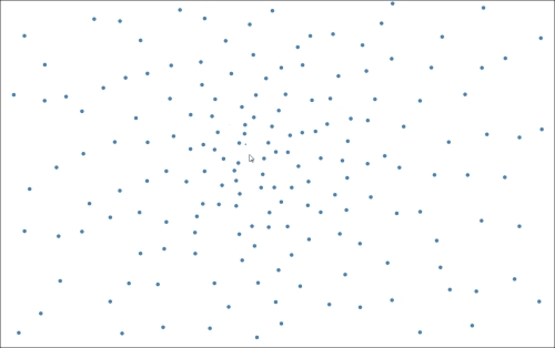
No Gravity or Charge

In the next mode, we will set the charge to a negative value while still keeping gravity to zero in order to generate a mutual repulsive force field:

function changeForce(charge, gravity) {
    force.charge(charge).gravity(gravity);
}
changeForce(-60, 0);

These lines tell force layout to apply -60 charge on each node and update the node's {x, y} coordinate accordingly, based on the simulation result on each tick. However, only doing this is still not enough to move the particles on SVG since the layout has no knowledge of the visual elements. Next, we need to write some code to connect the data that are being manipulated by force layout to our graphical elements. Following is the code to do that:

force.on("tick", function () {
        svg.selectAll("circle")
            .attr("cx", function (d) {return d.x;})
            .attr("cy", function (d) {return d.y;});
});

Here, we register a tick event listener function that updates all circle elements to its new position based on the force layout's calculation. Tick listener is triggered on each tick of the simulation. At each tick we set the cx and cy attribute to be the x and y values on d. This is because we have already bound the node object as datum to these circle elements, therefore, they already contain the new coordinates calculated by force layout. This effectively establishes force layout's control over all the particles.

Other than tick, force layout also supports some other events:

This force setting generates the following visual effect:

Mutual Repulsion

When we change the charge to a positive value, it generates mutual attraction among the particles:

function changeForce(charge, gravity) {
    force.charge(charge).gravity(gravity);
}
changeForce(60, 0);

This generates the following visual effect:

Mutual Attraction

When we turn on gravity and turn off charge then it generates a similar effect as the mutual attraction; however, you can notice the linear scaling of gravitational pull as the mouse moves away from the center:

function changeForce(charge, gravity) {
    force.charge(charge).gravity(gravity);
}
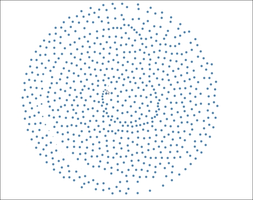
changeForce(0, 0.02);

With gravity alone this recipe generates the following effect:

Gravity

Finally, we can turn on both gravity and mutual repulsion. The result is an equilibrium of forces that keeps all particles somewhat stable neither escaping the layout nor colliding with each other:

function changeForce(charge, gravity) {
    force.charge(charge).gravity(gravity);
}
changeForce(-30, 0.1);

Here is what this force equilibrium looks like:

Gravity with Repulsion