Variational Autoencoders

An autoencoder is a model that tries to make its output equal to its input. You train it on a library of samples and adjust the model parameters so that on every sample the output is as close as possible to the input.

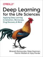
That sounds trivial. Can’t it just learn to pass the input directly through to the output unchanged? If that were actually possible it would indeed be trivial, but autoencoders usually have architectures that make it impossible. Most often this is done by forcing the data to go through a bottleneck, as shown in Figure 9-1. For example, the input and output might each include 1,000 numbers, but in between would be a hidden layer containing only 10 numbers. This forces the model to learn how to compress the input samples. It must represent 1,000 numbers worth of information using only 10 numbers.

Figure 9-1. Structure of a variational autoencoder.

If the model needed to handle arbitrary inputs, that would be impossible. You can’t throw out 99% of the information and still reconstruct the input! But we don’t care about arbitrary inputs, only the specific ones in the training set (and others that resemble them). Of all possible images, far less than 1% look anything like cats. An autoencoder doesn’t need to work for all possible inputs, only ones that are drawn from a specific probability distribution. It needs to learn the “structure” of that distribution, figure out how to represent the distribution using much less information, and then be able to reconstruct the samples based on the compressed information.

Now let’s take the model apart. The middle layer, the one that serves as the bottleneck, is called the latent space of the autoencoder. It is the space of compressed representations of samples. The first half of the autoencoder is called the encoder. Its job is to take samples and convert them to compressed representations. The second half is called the decoder. It takes compressed representations in the latent space and converts them back into the original samples.

This gives us our first clue about how autoencoders could be used for generative modeling. The decoder takes vectors in the latent space and converts them into samples, so we could take random vectors in the latent space (picking a random value for each component of the vector) and pass them through the decoder. If everything goes well, the decoder should produce a completely new sample that still resembles the ones it was trained on.

This sort of works, but not very well. The problem is that the encoder may only produce vectors in a small region of the latent space. If we pick a vector anywhere else in the latent space, we may get an output that looks nothing like the training samples. In other words, the decoder has only learned to work for the particular latent vectors produced by the encoder, not for arbitrary ones.

A variational autoencoder (VAE) adds two features to overcome this problem. First, it adds a term to the loss function that forces the latent vectors to follow a specified distribution. Most often they are constrained to have a Gaussian distribution with a mean of 0 and a variance of 1. We don’t leave the encoder free to generate vectors wherever it wants. We force it to generate vectors with a known distribution. That way, if we pick random vectors from that same distribution, we can expect the decoder to work well on them.

Second, during training we add random noise to the latent vector. The encoder converts the input sample to a latent vector, and then we randomly change it a little bit before passing it through the decoder, requiring the output to still be as close as possible to the original sample. This prevents the decoder from being too sensitive to the precise details of the latent vector. If we only change it by a little bit, the output should only change by a little bit.

These changes do a good job of improving the results. VAEs are a popular tool for generative modeling: they produce excellent results on many problems.

Generative Adversarial Networks

A generative adversarial network (GAN) has much in common with a VAE. It uses the same exact decoder network to convert latent vectors into samples (except in a GAN, it is called the generator instead of the decoder). But it trains that network in a different way. It works by passing random vectors into the generator and directly evaluating the outputs on how well they follow the expected distribution. Effectively, you create a loss function to measure how well the generated samples match the training samples, then use that loss function to optimize the model.

That sounds simple for a few seconds, until you think about it and realize it isn’t simple at all. Could you write a loss function to measure how well an image resembles a cat? No, of course not! You wouldn’t know where to begin. So, instead of asking you to come up with that loss function yourself, a GAN learns the loss function from the data.

As shown in Figure 9-2, a GAN consists of two parts. The generator takes random vectors and generates synthetic samples. The second part, called the discriminator, tries to distinguish the generated samples from real training samples. It takes a sample as input and outputs a probability that this is a real training sample. It acts as a loss function for the generator.

Figure 9-2. Structure of a generative adversarial network.

Both parts are trained simultaneously. Random vectors are fed into the generator, and the output is fed into the discriminator. The parameters of the generator are adjusted to make the discriminator’s output as close as possible to 1, while the parameters of the discriminator are adjusted to make its output as close as possible to 0. In addition, real samples from the training set are fed into the discriminator, and its parameters are adjusted to make the output close to 1.

This is the “adversarial” aspect. You can think of it as a competition between the generator and discriminator. The discriminator is constantly trying to get better at distinguishing real samples from fake ones. The generator is constantly trying to get better at fooling the discriminator.

Like VAEs, GANs are a popular type of generative model that produces good results on many problems. The two types of models have distinct strengths and weaknesses. Very roughly speaking, one might say that GANs tend to produce higher-quality samples, while VAEs tend to produce higher-quality distributions. That is, individual samples generated by a GAN will more closely resemble training samples, while the range of samples generated by a VAE will more closely match the range of training samples. Don’t take that statement too literally, though. It all depends on the particular problem and the details of the model. Also, countless variations on both approaches have been proposed. There even are models that combine a VAE with a GAN to try to get the best features of both. This is still a very active field of research, and new ideas are published frequently.

Applications of Generative Models in the Life Sciences

Now that we’ve introduced you to the basics of deep generative models, let’s start talking about applications. Broadly speaking, generative models bring a few superpowers to the table. First, they allow for a semblance of “creativity.” New samples can be generated according to the learned distribution. This allows for a powerful complement to a creative process that can tie into existing efforts in drug or protein design. Second, being able to model complex systems accurately with generative models could allow scientists to build an understanding of complex biological processes. We’ll discuss these ideas in more depth in this section.

Conclusion

While generative models provide an interesting means of producing ideas for new molecules, some key issues still need to be resolved to ensure their general applicability. The first is ensuring that the generated molecules will be chemically stable and that they can be physically synthesized. One current method to assess the quality of molecules produced by a generative model is to observe the fraction of the generated molecules that obey standard rules of chemical valence—in other words, ensuring that each carbon atom has four bonds, each oxygen atom has two bonds, each fluorine atom has one bond, and so on. These factors become especially important when decoding from a latent space with a SMILES representation. While a generative model may have learned the grammar of SMILES, there may be nuances that are still missing.

The fact that a molecule obeys standard rules of valence does not necessarily ensure that it will be chemically stable. In some cases, a generative model may produce molecules containing functional groups that are known to readily decompose. As an example, consider the molecule in Figure 9-4. The functional group highlighted in the circle, known as a hemiacetal, is known to readily decompose.

Figure 9-4. A molecule containing an unstable group.

In practice, the probability of this molecule existing and being chemically stable is very small. There are dozens of chemical functionalities like this which are known to be unstable or reactive. When synthesizing molecules in a drug discovery project, medicinal chemists know to avoid introducing these functional groups. One way of imparting this sort of “knowledge” to a generative model is to provide a set of filters that can be used to postprocess the model output and remove molecules that may be problematic. In Chapter 11, we will provide a further discussion of some of these filters and how they are used in virtual screening. Many of the same techniques used to identify potentially problematic screening compounds can also be used to evaluate virtual molecules that are created by a generative model.

In order to test the biological activity of a molecule produced by a generative model, that molecule must first be synthesized by a chemist. The science of organic chemical synthesis has a rich history going back more than one hundred years. In this time, chemists have developed thousands of chemical reactions to synthesize drugs and drug-like molecules. The synthesis of a drug-like molecule typically requires somewhere between 5 and 10 chemical reactions, often referred to as “steps.” While some drug-like molecules can be readily synthesized, the synthetic route to more complex drug molecules may require more than 20 steps. Despite more than 50 years of work on automating the planning of organic syntheses, much of the process is still driven by human intuition followed by trial and error.

Fortunately, recent developments in deep learning are providing new ways of planning the synthesis of drug-like molecules. A number of groups have published methods that use deep learning to propose routes that can be used to synthesize molecules. As input, the model is given a molecule, often referred to as a product, and the set of steps that were used to synthesize that molecule. By training with thousands of product molecules and the steps used for synthesis, a deep neural network is able to learn the relationship between product molecules and reaction steps. When presented with a new molecule, the model suggests a set of reactions that could be used to synthesize the molecule. In one test, the synthetic routes produced by these models were presented to human chemists for evaluation. These evaluators felt that the routes generated by the models were comparable in quality to routes generated by human chemists.

The application of deep learning to organic synthesis is a relatively new field. It is hoped that the field will continue to evolve and that these models become an important tool for organic chemists. One can imagine a day in the not too distant future where these synthesis planning capabilities could be paired with robotic automation to create a fully automated platform. However, there are difficulties to overcome.

One potential roadblock in the broad adoption of deep learning in organic synthesis is data availability. The majority of the information used to train these models is in databases which are the property of a small number of organizations. If these organizations decide to only utilize this data for their internal efforts, the field will be left with very few alternatives.

Another factor that may limit the advance of generative models is the quality of the predictive models that are used to drive molecule generation. Regardless of the architecture used to develop a generative model, some function must be used to evaluate the generated molecules and to direct the search for new molecules. In some cases, we may be able to develop reliable predictive models. In other cases, the models may be less reliable. While we can test our models on external validation sets, it is often difficult to determine the scope of a predictive model. This scope, also known as the “domain of applicability,” is the degree to which one can extrapolate outside the molecules on which a model was trained. This applicability domain is not well defined, so it may be difficult to determine how well a model will work on novel molecules produced by a generative model.

Generative models are a relatively new technique, and it will be interesting to see how this field evolves in the coming years. As our ability to use deep learning to predict routes for organic synthesis and build predictive models improves, the power of generative models will continue to grow.