DNA, RNA, and Proteins

Even if you are not a biologist, at some point in your education you probably studied the basics of how genomes operate. We will first review the simplified picture of genomics that is usually taught in introductory classes. Then we will describe some of the ways in which the real world is more complicated.

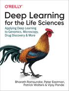
DNA is a polymer: a long chain of repeating units strung together. In the case of DNA, there are four units (called bases) that can appear: adenine, cytosine, guanine, and thymine, which are abbreviated as A, C, G, and T (see Figure 6-1). Nearly all the information about how to make a living organism is ultimately encoded in the specific pattern of these four repeating units that make up its genome.

Figure 6-1. Structure of a DNA molecule. It consists of two chains, each made of many A, C, G, and T bases. The two chains are complementary: every C in one chain is paired with a G in the other, and every A in one chain is paired with a T in the other. (Source: Wikimedia.)

If DNA is the software, proteins are the most important hardware. Proteins are tiny machines that do almost all the work in a cell. Proteins are also polymers, made up of repeating units called amino acids. There are 20 main amino acids, and their physical properties vary widely. Some are large while others are small. Some have an electric charge while others do not. Some tend to attract water while others tend to repel it. When just the right set of amino acids is strung together in just the right order, it will spontaneously fold up into a 3D shape, all the pieces positioned just right to let it function as a machine.

One of the main functions of DNA is to record the sequences of amino acids for an organism’s proteins. It does this in a simple, straightforward way. Particular stretches of DNA directly correspond to particular proteins. Each sequence of three DNA bases (called a codon) corresponds to one amino acid. For example, the pattern AAA indicates the amino acid lysine, while the pattern GCC indicates the amino acid alanine.

Going from DNA to protein involves another molecule, RNA, that serves as an intermediate representation to carry information from one part of the cell to another. RNA is yet another polymer and is chemically very similar to DNA. It too has four bases that can be chained together in arbitrary orders. To create a protein, the information must be copied twice. First the DNA sequence is transcribed into an equivalent RNA sequence, and then the RNA molecule is translated into a protein molecule. The RNA molecule that carries the information is called a messenger RNA, or mRNA for short.

This tells us how proteins get made, but not when. A human cell has many thousands of different proteins it can make. Surely it doesn’t just churn out copies of all of them, all the time? Clearly there must be some sort of regulatory mechanism to control which proteins get made when. In the conventional picture, this is done by special proteins called transcription factors (TFs). Each TF recognizes and binds to a particular DNA sequence. Depending on the particular TF and the location where it binds, it can either increase or decrease the rate at which nearby genes are transcribed. 

This gives a simple, easy-to-understand picture of how a genome works. The job of DNA is to encode proteins. Stretches of DNA (called genes) code for proteins using a simple, well-defined code. DNA is converted to RNA, which serves only as an information carrier. The RNA is then converted into proteins, which do all the real work. The whole process is very elegant, the sort of thing a talented engineer might have designed. And for many years, this picture was believed to be mostly correct. So, take a moment to enjoy it before we spoil the view by revealing that reality is actually far messier and far more complicated.

And Now for the Real World

Now it’s time to talk about how genomes really work. The picture described in the previous section is simple and elegant, but unfortunately it has little connection to reality. This section will go through a lot of information very quickly, but don’t worry about remembering or understanding all of it. The important thing is just to get a sense of the incredible complexity of living organisms. We will return to some of these subjects later in the chapter and discuss them in more detail.

Let’s begin by considering DNA molecules (called chromosomes). In bacteria, which have relatively small genomes, DNA exists as simple free-floating molecules. But eukaryotes (a group that includes amoebas, humans, and everything in between) have much larger genomes. To fit inside the cell, each chromosome must be packed into a very small space. This is accomplished by winding it around proteins called histones. But if all the DNA is tightly packed away, how can it be transcribed? The answer, of course, is that it can’t. Before a gene can be transcribed, the stretch of DNA containing it first must be unwound. How does the cell know which DNA to unwind? The answer is still poorly understood. It is believed to involve various types of chemical modification to the histone molecules, and proteins that recognize particular modifications. Clearly there is a regulatory mechanism involved, but many of the details are still unknown. We will return to this subject shortly.

DNA itself can be chemically modified through a process called methylation. The more highly a stretch of DNA is methylated, the less likely it is to be transcribed, so this is another regulatory mechanism the cell can use to control the production of proteins. But how does it control which regions of DNA are methylated? This too is still poorly understood.

In the previous section we said that a particular stretch of DNA corresponds to a particular protein. That is correct for bacteria, but in eukaryotes the situation is more complicated. After the DNA is transcribed into a messenger RNA, that RNA often is edited to remove sections and connect (or splice) the remaining parts (called exons) back together again. The RNA sequence that finally gets translated into a protein may therefore be different from the original DNA sequence. In addition, many genes have multiple splice variants—different ways of removing sections to form the final sequence. This means a single stretch of DNA can actually code for several different proteins!

Is all of this starting to sound very complicated? Well, keep reading, because we’ve barely started! Evolution selects for mechanisms that work, without any concern for whether they are simple or easy to understand. It leads to very complicated systems, and understanding them requires us to confront that complexity.

In the conventional picture RNA is viewed as just an information carrier, but even from the early days of genomics, biologists knew that was not entirely correct. The job of translating mRNA to proteins is performed by ribosomes, complicated molecular machines made partly of proteins and partly of RNA. Another key role in translation is performed by molecules called transfer RNAs (or tRNAs for short). These are the molecules that define the “genetic code,” recognizing patterns of three bases in mRNA and adding the correct amino acid to the growing protein. So, for over half a century we’ve known there were at least three kinds of RNA: mRNA, ribosomal RNA, and tRNA.

But RNA still had lots of tricks up its sleeve. It is a surprisingly versatile molecule. Over the last few decades, many other types of RNA have been discovered. Here are some examples:

• Micro RNAs (miRNAs) are short pieces of RNA that bind to a messenger RNA and prevent it from being translated into proteins. This is a very important regulatory mechanism in some types of animals, especially mammals.

• Short interfering RNA (siRNA) is another type of RNA that binds to mRNA and prevents it from being translated. It’s similar to miRNA, but siRNAs are double stranded (unlike miRNAs, which are single stranded), and some of the details of how they function are different. We will discuss siRNA in more detail later in the chapter.

• Ribozymes are RNA molecules that can act as enzymes to catalyze chemical reactions. Chemistry is the foundation of everything that happens in a living cell, so catalysts are vital to life. Usually this job is done by proteins, but we now know it sometimes is done by RNA.

• Riboswitches are RNA molecules that consist of two parts. One part acts as a messenger RNA, while the other part is capable of binding to a small molecule. When it binds, that can either enable or prevent translation of the mRNA. This is yet another regulatory mechanism by which protein production can be adjusted based on the concentration of particular small molecules in the cell.

Of course, all these different types of RNA must be manufactured, and the DNA must contain instructions on how to make them. So, DNA is more than just a string of encoded protein sequences. It also contains RNA sequences, plus binding sites for transcription factors and other regulatory molecules, plus instructions for how messenger RNAs should be spliced, plus various chemical modifications that influence how it is wound around histones and which genes get transcribed.

Now consider what happens after the ribosome finishes translating the mRNA into a protein. Some proteins can spontaneously fold into the correct 3D shape, but many others require help from other proteins called chaperones. It is also very common for proteins to need additional chemical modifications after they are translated. Then the finished protein must be transported to the correct location in the cell to do its job, and finally degraded when it is no longer needed. Each of these processes is controlled by additional regulatory mechanisms, and involves interactions with lots of other molecules.

If this all sounds overwhelming, that’s because it is! A living organism is far more complicated than any machine ever created by humans. The thought of trying to understand it should intimidate you!

But this is also why machine learning is such a powerful tool. We have huge amounts of data, generated by a process that is both mind-bogglingly complex and poorly understood. We want to discover subtle patterns buried in the data. This is exactly the sort of problem that deep learning excels at!

In fact, deep learning is uniquely well suited to the problem. Classical statistical techniques struggle to represent the complexity of the genome. They often are based around simplifying assumptions. For example, they look for linear relationships between variables, or they try to model a variable as depending on only a small number of other variables. But genomics involves complex nonlinear relationships between hundreds of variables: exactly the sort of relationship that can be effectively described by a deep neural network.

Transcription Factor Binding

As an example of applying deep learning to genomics, let’s consider the problem of predicting transcription factor binding. Recall that TFs are proteins that bind to DNA. When they bind, they influence the probability of nearby genes being transcribed into RNA. But how does a TF know where to bind? Like so much of genomics, this question has a simple answer followed by lots of complications.

To a first approximation, every TF has a specific DNA sequence called its binding site motif that it binds to. Binding site motifs tend to be short, usually 10 bases or less. Wherever a TF’s motif appears in the genome, the TF will bind to it.

In practice, though, motifs are not completely specific. A TF may be able to bind to many similar but not identical sequences. Some bases within the motif may be more important than others. This is often modeled as a position weight matrix that specifies how much preference the TF has for each possible base at each position within the motif. Of course, that assumes every position within the motif is independent, which is not always true. Sometimes even the length of a motif can vary. And although binding is primarily determined by the bases within the motif, the DNA to either side of it can also have some influence.

And that’s just considering the sequence! Other aspects of the DNA can also be important. Many TFs are influenced by the physical shape of the DNA, such as how tightly the double helix is twisted. If the DNA is methylated, that can influence TF binding. And remember that most DNA in eukaryotes is tightly packed away, wound around histones. TFs can only bind to the portions that have been unwound.

Other molecules also play important roles. TFs often interact with other molecules, and those interactions can affect DNA binding. For example, a TF may bind to a second molecule to form a complex, and that complex then binds to a different DNA motif than the TF would on its own.

Biologists have spent decades untangling these details and designing models for TF binding. Instead of doing that, let’s see if we can use deep learning to learn a model directly from data.

A Convolutional Model for TF Binding

For this example, we will use experimental data on a particular transcription factor called JUND. An experiment was done to identify every place in the human genome where it binds. To keep things manageable, we only include the data from chromosome 22, one of the smallest human chromosomes. It is still over 50 million bases long, so that gives us a reasonable amount of data to work with. The full chromosome has been split up into short segments, each 101 bases long, and each segment has been labeled to indicate whether it does or does not include a site where JUND binds. We will try to train a model that predicts those labels based on the sequence of each segment.

The sequences are represented with one-hot encoding. For each base we have four numbers, of which one is set to 1 and the others are set to 0. Which of the four numbers is set to 1 indicates whether the base is an A, C, G, or T.

To process the data we will use a convolutional neural network, just like we did for recognizing handwritten digits in Chapter 3. In fact, you will see the two models are remarkably similar to each other. This time we will use 1D convolutions, since we are dealing with 1D data (DNA sequences) instead of 2D data (images), but the basic components of the model will be the same: inputs, a series of convolutional layers, one or more dense layers to compute the output, and a cross entropy loss function.

Let’s start by creating a TensorGraph and defining the inputs:

model = dc.models.TensorGraph(batch_size=1000)
features = layers.Feature(shape=(None, 101, 4))
labels = layers.Label(shape=(None, 1))
weights = layers.Weights(shape=(None, 1))

Notice the sizes of the inputs. For each sample, we have a feature vector of size 101 (the number of bases) by 4 (the one-hot encoding of each base). We also have a single number for the label (either 0 or 1, to indicate whether it contains a binding site) and a single number for the weight. Using weights in the loss function is critical for this example, because the data is very unbalanced. Less than 1% of all samples include a binding site. That means the model could trivially get better than 99% accuracy by just outputting 0 for every sample. We prevent this by giving the positive samples higher weights than the negative ones.

Next we create a stack of three convolutional layers, all with identical parameters:

prev = features
for i in range(3):
  prev = layers.Conv1D(filters=15, kernel_size=10,
                       activation=tf.nn.relu, padding='same',
                       in_layers=prev)
  prev = layers.Dropout(dropout_prob=0.5, in_layers=prev)

We specify 10 for the width of the convolutional kernels, and that each layer should include 15 filters (that is, outputs). The first layer takes the raw features (four numbers per base) as input. It looks at spans of 10 consecutive bases, so 40 input values in total. For each span, it multiplies those 40 values by a convolutional kernel to produce 15 output values. The second layer again looks at spans of 10 bases, but this time the inputs are the 15 values computed by the first layer. It computes a new set of 15 values for each base, and so on.

To prevent overfitting, we add a dropout layer after each convolutional layer. The dropout probability is set to 0.5, meaning that 50% of all output values are randomly set to 0.

Next we use a dense layer to compute the output:

logits = layers.Dense(out_channels=1, in_layers=layers.Flatten(prev))
output = layers.Sigmoid(logits)
model.add_output(output)

We want the output to be between 0 and 1 so we can interpret it as the probability a particular sample contains a binding site. The dense layer can produce arbitrary values, not limited to any particular range. We therefore pass it through a logistic sigmoid function to compress it to the desired range. The input to this function is often referred to as logits. The name refers to the mathematical logit function, which is the inverse function of the logistic sigmoid.

Finally, we compute the cross entropy for each sample and multiply by the weights to get the loss:

loss = layers.SigmoidCrossEntropy(in_layers=[labels, logits])
weighted_loss = layers.WeightedError(in_layers=[loss, weights])
model.set_loss(weighted_loss)

Notice that for reasons of numerical stability, the cross entropy layer takes logits as input instead of the output of the sigmoid function.

Now we are ready to train and evaluate the model. We use ROC AUC as our evaluation metric. After every 10 epochs of training, we evaluate the model on both the training and validation sets:

train = dc.data.DiskDataset('train_dataset')
valid = dc.data.DiskDataset('valid_dataset')
metric = dc.metrics.Metric(dc.metrics.roc_auc_score)
for i in range(20):
  model.fit(train, nb_epoch=10)
  print(model.evaluate(train, [metric]))
  print(model.evaluate(valid, [metric]))

The result is shown in Figure 6-2. The validation set performance peaks at about 0.75 after 50 epochs, then decreases slightly. The training set performance continues to increase, eventually leveling off at around 0.87. This tells us that training beyond 50 epochs just leads to overfitting, and we should halt training at that point:

Figure 6-2. Evolution of ROC AUC scores during training for the training set (dashed) and validation set (solid).

A ROC AUC score of 0.75 is not bad, but also not wonderful. Possibly we could increase it by improving the model. There are lots of hyperparameters we could try changing: the number of convolutional layers, the kernel width for each layer, the number of filters in each layer, the dropout rate, etc. We could try lots of combinations for them, and we might find one with better performance.

But we also know there are fundamental limits to how well this model can ever work. The only input it looks at is the DNA sequence, and TF binding also depends on lots of other factors: accessibility, methylation, shape, the presence of other molecules, etc. Any model that ignores those factors will be limited in how accurate its predictions can ever be. So now let’s try adding a second input and see if it helps.

Chromatin Accessibility

The name chromatin refers to everything that makes up a chromosome: DNA, histones, and various other proteins and RNA molecules. Chromatin accessibility refers to how accessible each part of the chromosome is to outside molecules. When the DNA is tightly wound around histones, is becomes inaccessible to transcription factors and other molecules. They cannot reach it, and the DNA is effectively inactive. When it unwinds from the histones, it becomes accessible again and resumes its role as a central part of the cell’s machinery.

Chromatin accessibility is neither uniform nor static. It varies between types of cells and stages of a cell’s life cycle. It can be affected by environmental conditions. It is one of the tools a cell uses to regulate the activity of its genome. Any gene can be turned off by packing away the area of the chromosome where it is located.

Accessibility also is constantly changing as DNA winds and unwinds in response to events in the cell. Instead of thinking of accessibility as a binary choice (accessible or inaccessible), it is better to think of it as a continuous variable (what fraction of the time each region is accessible).

The data we analyzed in the last section came from experiments on a particular kind of cell called HepG2. The experiments identified locations in the genome where the transcription factor JUND was bound. The results were influenced by chromatin accessibility. If a particular region is almost always inaccessible in HepG2 cells, the experiment was very unlikely to find JUND bound there, even if the DNA sequence would otherwise be a perfect binding site. So, let’s try incorporating accessibility into our model.

First let’s load some data on accessibility. We have it in a text file where each line corresponds to one sample from our dataset (a 101-base stretch of chromosome 22). A line contains the sample ID followed by a number that measures how accessible that region tends to be in HepG2 cells. We’ll load it into a Python dictionary:

span_accessibility = {}
for line in open('accessibility.txt'):
  fields = line.split()
  span_accessibility[fields[0]] = float(fields[1])

Now to build the model. We will use almost exactly the same model as in the previous section with just two minor changes. First, we need a second feature input for the accessibility values. It has one number for each sample:

accessibility = layers.Feature(shape=(None, 1))

Now we need to incorporate the accessibility value into the calculation. There are many ways we might do this. For the purposes of this example, we will use a particularly simple method. In the previous section, we flattened the output of the last convolution layer, then used it as the input to a dense layer that calculated the output.

logits = layers.Dense(out_channels=1, in_layers=layers.Flatten(prev))

This time we will do the same thing, but also append the accessibility to the output of the convolution:

prev = layers.Concat([layers.Flatten(prev), accessibility])
logits = layers.Dense(out_channels=1, in_layers=prev)

That’s all there is to the model! Now it’s time to train it.

At this point we run into a difficulty: our model has two different Feature layers! Up until now, our models have had exactly one Feature layer, one Label layer, and possibly one Weights layer. We trained them by calling fit(dataset), which automatically connected the correct data to each layer: the dataset’s X field for the features, y for the labels, and w for the weights. But that clearly can’t work when the model has more than one set of features.

This situation is handled by using a more advanced feature of DeepChem. Instead of passing a dataset to the model, we can write a Python generator function that iterates over batches. Each batch is represented by a dictionary whose keys are input layers, and whose values are the NumPy arrays to use for them:

def generate_batches(dataset, epochs):
  for epoch in range(epochs):
    for X, y, w, ids in dataset.iterbatches(batch_size=1000,
                                            pad_batches=True):
      yield {
	features: X,
	accessibility: np.array([span_accessibility[id] for id in ids]),
	labels: y,
	weights: w
      }

Notice how the dataset takes care of iterating through batches for us. It provides the data for each batch, from which we can construct whatever inputs the model requires.

Training and evaluation now proceed exactly as before. We use alternate forms of the methods that take a generator instead of a dataset:

for i in range(20):
  model.fit_generator(generate_batches(train, 10))
  print(model.evaluate_generator(generate_batches(train, 1), [metric],
                                 labels=[labels], weights=[weights]))
  print(model.evaluate_generator(generate_batches(valid, 1), [metric],
                                 labels=[labels], weights=[weights]))

The result is shown in Figure 6-3. Both the training and validation set scores are improved compared to the model that ignored chromatin accessibility. ROC AUC score now reaches 0.91 for the training set and 0.80 for the validation set.

Figure 6-3. Evolution of ROC AUC scores during training for the training set (dashed) and validation set (solid) when including chromatin accessibility as an input.

RNA Interference

For our final example, let’s turn to RNA. Much like DNA, this is a polymer composed of four repeating units called bases. In fact, three of the four bases are almost identical to their DNA versions, differing only in having one extra oxygen atom. The fourth base is a little more different. In place of thymine (T), RNA has a base called uracil (U). When a DNA sequence is transcribed into RNA, every T is replaced by a U.

The bases G and C are complementary to each other, in the sense that they have a strong tendency to bond to each other. Likewise, the bases A and T (or U) are complementary. If you have two strands of DNA or RNA, and every base in one is complementary to the corresponding base in the other, the two strands will tend to stick together. This fact plays a key role in lots of biological processes, including both transcription and translation, as well as DNA replication when a cell is dividing.

It also is central to something called RNA interference.  This phenomenon was only discovered in the 1990s, and the discovery led to a Nobel Prize in 2006. A short piece of RNA whose sequence is complementary to part of a messenger RNA can bind to that mRNA. When this happens, it “silences” the mRNA and prevents it from being translated into a protein. The molecule that does the silencing is called a short interfering RNA (siRNA).

Except there is much more to the process than that. RNA interference is a complex biological mechanism, not just a side effect of two isolated RNA strands happening to stick together. It begins with the siRNA binding to a collection of proteins called the RNA-induced silencing complex (RISC). The RISC uses the siRNA as a template to search out matching mRNAs in the cell and degrade them. This serves both as a mechanism for regulating gene expression and as a defense against viruses.

It also is a powerful tool for biology and medicine. It lets you temporarily “turn off” any gene you want. You can use it to treat a disease, or to study what happens when a gene is disabled. Just identify the mRNA you want to block, select any short segment of it, and create a siRNA molecule with the complementary sequence.

Except that (of course!) it isn’t as simple as that. You can’t really just pick any segment of the mRNA at random, because (of course!) RNA molecules aren’t just abstract patterns of four letters. They are physical objects with distinct properties, and those properties depend on the sequence. Some RNA molecules are more stable than others. Some bind their complementary sequences more strongly than others. Some fold into shapes that make it harder for the RISC to bind them. This means that some siRNA sequences work better than others, and if you want to use RNA interference as a tool, you need to know how to select a good one!

Biologists have developed lots of heuristics for selecting siRNA sequences. They will say, for example, that the very first base should be either an A or G, that G and C bases should make up between 30% and 50% of the sequence, and so on. These heuristics are helpful, but let’s see if we can do better using machine learning.

We’ll train our model using a library of 2,431 siRNA molecules, each 21 bases long.¹ Every one of them has been tested experimentally and labeled with a value between 0 and 1, indicating how effective it is at silencing its target gene. Small values indicate ineffective molecules, while larger values indicate more effective ones. The model takes the sequence as input and tries to predict the effectiveness.

Here is the code to build the model:

model = dc.models.TensorGraph()
features = layers.Feature(shape=(None, 21, 4))
labels = layers.Label(shape=(None, 1))
prev = features
for i in range(2):
  prev = layers.Conv1D(filters=10, kernel_size=10,
                       activation=tf.nn.relu, padding='same',
                       in_layers=prev)
  prev = layers.Dropout(dropout_prob=0.3, in_layers=prev)
output = layers.Dense(out_channels=1, activation_fn=tf.sigmoid,
                      in_layers=layers.Flatten(prev))
model.add_output(output)
loss = layers.ReduceMean(layers.L2Loss(in_layers=[labels, output]))
model.set_loss(loss)

This is very similar to the model we used for TF binding, with just a few differences. Because we are working with shorter sequences and training on less data, we have reduced the size of the model. There are only 2 convolutional layers, and 10 filters per layer instead of 15. There also is no need for weights, since we want every sample to contribute equally during optimization.

We also use a different loss function. The model for TF binding was a classification model. Every label was either 0 or 1, and we tried to predict which of those two discrete values it was. But this one is a regression model. The labels are continuous numbers, and the model tries to match them as closely as possible. We therefore use the $L_2$ distance as our loss function, which tries to minimize the mean squared difference between the true and predicted labels.

Here is the code to train the model:

train = dc.data.DiskDataset('train_siRNA')
valid = dc.data.DiskDataset('valid_siRNA')
metric = dc.metrics.Metric(dc.metrics.pearsonr, mode='regression')
for i in range(20):
  model.fit(train, nb_epoch=10)
  print(model.evaluate(train, [metric]))
  print(model.evaluate(valid, [metric]))

For TF binding, we used ROC AUC as our evaluation metric, which measures how accurately the model can divide the data into two classes. That is appropriate for a classification problem, but it doesn’t make sense for a regression problem, so instead we use the Pearson correlation coefficient. This is a number between –1 and 1, where 0 means the model provides no information at all and 1 means the model perfectly reproduces the experimental data.

The result is shown in Figure 6-4. The validation set score peaks at 0.65 after 50 epochs. The training set score continues to increase, but since there is no further improvement to the validation set score this is just overfitting. Given the simplicity of the model and the limited amount of training data, a correlation coefficient of 0.65 is quite good. More complex models trained on larger datasets do slightly better, but this is already very respectable performance.

Figure 6-4. Evolution of the Pearson correlation coefficient during training for the training set (dashed) and validation set (solid).

Conclusion

A genome is an enormously complicated machine, with a vast number of parts all working together to direct and carry out the manufacture of proteins and other molecules. Deep learning is a powerful tool for studying it. Neural networks can pick out the subtle patterns in genomic data, providing insight into how the genome functions as well as making predictions about it.

Even more than most other areas of the life sciences, genomics produces huge amounts of experimental data. For example, a single human genome sequence includes more than six billion bases. Traditional statistical techniques struggle to find the signal buried in all that data. They often require simplifying assumptions that do not reflect the complexity of genomic regulation. Deep learning is uniquely suited to processing this data and advancing our understanding of the core functions of living cells.