In Chapter 6 we considered the matched filter reception of baseband pulses in an AWGN channel, and the ISI due to band‐limiting and multipath. We also considered pulse shaping and other techniques for ISI mitigation. In this chapter, we will consider the details of the receiver design for the reception of sequences of M‐ary symbols and the resulting error probability in a baseband channel in the presence of AWGN.
7.1 Introduction
Consider a digital communication system with a block diagram as shown in Figure 7.1, where a message source emits every T seconds one symbol from an alphabet of M symbols, m1, m2,…, mM with a priory probabilities p1, p2,…., pM. In most cases of interest, M symbols of the alphabet are equally likely:
(7.1)
Figure 7.1 Block Diagram of a Baseband Digital Communication System.
Transmitter converts the message source output mi into a distinct electrical signal si(t), suitable for transmission over the channel. Hence the transmission of digital information is accomplished by using one of the M signals every T seconds:
(7.2)
The energy of the real‐valued energy signal si(t) over the symbol duration T:
Depending on the application of interest, a priori probabilities and the symbol energies of the M signals may be the same. However, we assume that they are not the same. As an example of M‐ary transmission, 8‐PAM is shown in Figure 6.24.
In this so‐called M‐ary transmission, si(t) is used to transmit the information carried by the symbol mi, consisting of k = log2M bits, in the symbol duration T. Noting that a symbol mi is k = log2M bits long, the symbol duration is T = kTb, where Tb denotes the bit duration, and the symbol energy is given by . The symbol duration and the symbol rate are related to the bit duration and the bit rate as follows:
(7.4)
where Rb = 1/Tb denotes the bit rate in bits/s and R = 1/T is the symbol rate in symbols/s.
The channel depicted in Figure 7.1 is assumed to be linear and to have sufficiently wide bandwidth for transmission of si(t) so as to cause minimum distortion and ISI. In the AWGN channel, where the noise w(t) has zero mean and a one‐sided PSD of N0, the received signal may be written as
A receiver may be subdivided into two functionalities; a signal demodulator and a decoder (detector). The demodulator converts the received signal x(t) into an N‐dimensional observation vector x = [x1 x2 ….. xN] with orthogonal components, where N denotes the dimension of the transmitted signal. Two realizations of the signal demodulator, as a correlator or a matched filter, perform identically at the sampling instants as already demonstrated in Chapter 6. Based on the observation vector x and some preset threshold levels, the detector estimates the transmitted symbol. Hence, given the received noisy signal (7.5), a receiver makes a decision as to which of the M signals, hence symbols, is transmitted in the considered symbol duration. A receiver is desired to be optimum in the sense that it minimizes the probability of making an error in estimating the transmitted symbol mi. For example, Figure 7.2 shows the transmission of a 4‐ary signal with dimension N = 2. The received signal given by (7.5) is decomposed by the demodulator into two orthogonal components x1(t) and x2(t) along the orthonormal basis functions ϕ1(t) and ϕ2(t) to enable the detector to make the best estimate of the transmitted symbol. [1][2][3][4]
Figure 7.2 Signal Constellation at the Receiver Input and the Observation Vector at the Demodulator Output for a 4‐ary Signal of Dimension N = 2.
In this chapter, we will consider the design and the performance evaluation of optimum receivers in an AWGN channel based on the assumption that no ISI or distortion is introduced by the channel.
7.2 Geometric Representation of Signals
Each signal in {si(t), i = 1,2,..,M} is defined by the signal vectors {si, i = 1,2,…,M} in an N‐dimensional Euclidean signal space, with N mutually perpendicular axes, ϕ1, ϕ2…,ϕN:
(7.6)
In other words, any M‐ary signal may be expressed as a linear combination of N orthonormal basis functions, {ϕi(t), i = 1,2,…,N}, where N ≤ M: [1][3]
The implementation of a synthesizer for generating si(t) in terms of its orthogonal components and of an analyser for determining the orthogonal components of si(t) are shown in Figure 7.3.
Figure 7.3 Geometric Representation of the Signal si(t). a) synthesizer for generating the signal si(t), and b) analyzer for obtaining the orthogonal signal components.
Length (norm, absolute value) of a signal vector si may be expressed as
(7.8)
The energy of a signal defined by (7.3) can be shown to be equal to the square of its norm:
(7.9)
The square of the Euclidean distance between the signals si(t) and sk(t) is given by
As shown in Figure 7.3b, a demodulator decomposes the received signal x(t) given by (7.5) into N orthogonal components. Using the geometric signal representation given by (7.7), the received signal x(t) is applied to the input of the demodulator which may be implemented as a bank of correlators/matched filters:
The last term in (7.19) is called the remainder noise and represents the noise which is orthogonal to the space spanned by {ϕi(t), i = 1,2,…N}. Note that the set of basis vectors {ϕi(t), i = 1,2,…N} span the signal space but not the noise space. According to the so‐called theorem of irrelevance, for signal demodulation in an AWGN channel, only the projections of the noise onto the basis functions of the signal set affect the sufficient statistics for the detection problem; the remainder noise is irrelevant. This implies that the decoder does not need the knowledge of the remainder noise to make an estimate as to which signal is transmitted.
Figure 7.6 Decision Regions Z1 and Z2 for Matched Filter Reception of a Binary PAM Signal.
Figure 7.7 Equivalence of matched‐filter and correlator implementations. Correlator and matched filter outputs are identical at the sampling time t = T.
Figure 7.8 Block Diagram of a Demodulator Implemented as a Bank of Matched Filters.
7.3.1 Coherent Detection of Signals in AWGN Channels
The observation vector at the demodulator output, which may be written as , is perturbed by the presence of the additive noise vector w. The noise vector , consisting of the projections of w(t) along the basis functions, does not contain the remainder noise and yet provides sufficient statistics for the detection process. Since noise components are circularly symmetric Gaussian random variables with zero mean and variance N0/2, the orientation of w is completely random. The signal vector may be represented as the transmitted signal point in a Euclidean space of dimension N ≤ M. The set of signal points {si}, i = 1,2,..,M are called as the signal constellation. Similarly, the received signal points are represented by the observation vector x in the same Euclidean space. A received signal point wanders around the message point randomly, lying anywhere inside a Gaussian distributed noise cloud, centred on the message point as shown pictorially in Figure 7.9. As the noise variance increases (Eb/N0 decreases), the cloud of 100 ksamples of noise becomes larger and the Euclidean distance between the observation and signal vectors increases. This can force the detector to make an erroneous estimate of the transmitted symbol.
Figure 7.9 Effect of Noise Perturbation on the Location of the Observation Vector in the Signal‐Space for Eb/N0 = 10 dB and 15 dB. Simulation is carried out with 100 ksamples of complex Gaussian noise.
Given the observation vector x, the decoder performs a mapping from x to an estimate of the transmitted symbol, mi, in a way that would minimize the probability of error in the decision‐making process. Given the observation vector x, the probability of error, when mi is transmitted, may be written as
where denotes the a priori probability of transmitting the symbol mi. On the other hand, shows the probability that, based on a given observation vector at the decoder input, the decoder estimates as mi being transmitted.
7.3.1.1 Optimum Decision Rule
Having formulated by (7.27), the probability of error in the detection process, we now consider minimizing the error probability. The maximum a posteriori probability (MAP) rule is an optimum decision rule which minimizes the probability of error in mapping each given observation vector x into a decision. Minimizing the error probability is equivalent to maximizing in (7.27). Hence, the detector estimates the transmitted symbol as follows: [2]
is maximum for k = i. Note that f(x|mk) denotes the conditional pdf of x, when mk is sent by the transmitter. Also note that f(x), the pdf of x,
(7.31)
is independent of the transmitted symbol mi.
For binary signaling with given a priori probabilities p(m1) and p(m2), the MAP decoding rule, which was already introduced in Example 6.4, may be based on the likelihood (or log‐likelihood) ratio test in order to estimate the transmitted symbol: [3]
If the likelihood of transmitting m1 is higher than for m2, then the log‐likelihood ratio (7.32) will be positive and the detector will decide that is transmitted. Otherwise, the detector will declare that m2 is sent. Therefore, L(m|x) has a soft value and its sign provides the hard decision as to m1 or m2 is transmitted:
(7.34)
The magnitude of L(m|x) represents the reliability of the decision. For example, the decoder is more confident to declare if L(m|x) is equal to 0.8 compared to 0.3.
If the source symbols are equiprobable that is, , then the MAP decoding, which is based on , may be accomplished by using only f(x|mk) since
(7.35)
Therefore, for the special case of equal symbol probabilities, the MAP decoding rule given by (7.30) simply reduces to
(7.36)
This is referred to as the maximum likelihood (ML) decoding rule and is implemented as a ML decoder. Note that the knowledge of f(x|mk) is already available at the demodulator output, as given by (7.26). A ML decoder calculates the likelihood functions for all possible message points, compares them, and then decides in favour of the one with maximum likelihood.
For binary signalling, the probabilities of transmitting m1 and m2 are the same, that is, . Then, in (7.33) and the MAP decoding rule reduces to the ML decoding rule:
(7.37)
For example, consider that antipodal signals s1 and s0 of equal energies Eb are used for the transmission of the binary symbols m1 and m0 with unequal a priori transmission probabilities in an AWGN channel. The observation vector at the matched‐filter output is given by
where n(T) has zero mean and variance σ2 = N0/2. Noting that the observation vector x has a dimension of N = 1 in antipodal signaling, the log‐likelihood ratio reduces to
The optimum threshold level in (7.40) is identical to (6.46) and minimizes the probability of error. The minimum probability of error may then be written as (see (6.41))
For the special case where , the optimum threshold becomes λopt = 0 and the corresponding error probability reduces to
(7.42)
For example, let the received signal level be x = 0.02 (see (7.38)), σ2 = 1, Eb = 10 and p1 = 0.3. From (7.39),
(7.43)
the negative sign of L(m|x) implies that MAP decoder decides (hard decision). The absolute value shows the confidence level in estimating the transmitted symbol. This is in agreement with the fact that the received signal level x = 0.02 is lower than the optimum threshold level
(7.44)
The corresponding error probability is found from (7.41) to be .
7.3.1.2 Geometrical Interpretation of Signal Space for MLD
In case where the a priori probabilities of are not equal to each other, the MAP decoding rule leads to minimum error probability if the decision regions are defined by the optimum threshold levels given by (7.40). For equiprobable signals, the MAP decoding reduces to MLD, where the decision regions are defined by the threshold levels that bisect the Euclidean distances between the signal points. To have a better feeling about the MLD, let Z denote the N‐dimensional observation space of all possible observation vectors x and the observation space is partitioned into M‐decision regions, Z1, Z2,…, ZM, corresponding to M symbols likely to be transmitted. Since the threshold levels bisect the Euclidean distances between the signal points, the message points and the observation space are equally distributed between them. As an example, Figure 7.11 shows the signal points and the observation space for M = 4 equal energy signals with identical a priori transmission probabilities. According to MLD decision rule, the observation vector x lies in region Zi if the likelihood function f(x|mk) is maximum for k = i (see (7.26)). In other words, Zi is chosen such that is minimized for k = i. MLD decision rule then estimates the signal with minimum Euclidean distance to the observation point as the most likely transmitted signal.
Figure 7.11 The Observation Space with Signal Points and Decision Regions for the Case When Dimensionality is N = 2 and the Number of Signal Points is M = 4. M transmitted symbols are assumed to be equally likely and have equal energies Es.
To elaborate this, let us expand the square‐Euclidean distance given by (7.26):
(7.60)
The first term in (7.60) may be ignored since, being independent of the transmitted signal, plays no role in estimating the transmitted signal. Noting that denotes the energy of the signal sk, the MLD decision rule (7.60) may be rephrased as: Observation vector x lies in region Zi (the ML decoder chooses ) if
Figure 7.12 shows the implementation diagram of an optimum detector defined by (7.61). The accumulators are digital integrators and compute . If signals have equal energies, then the term Ek/2 may be ignored.
Note that the complex Gaussian noise is circularly symmetric in all directions in the signal space and the probability of error depends only on the Euclidean distances between the message points in the constellation diagram. This leads us to the principle of rotational invariance which states that if a signal constellation is rotated by an orthonormal transformation, then the Pe incurred in MLD in an AWGN channel is unchanged. Figure 7.13 shows an example to the principle of rotational invariance for a signal defined by N = 2 and M = 4. [2]
Figure 7.13 Demonstration of the Principle of Rotational Invariance. Rotation of the constellation does not change the error probability.
If a signal constellation is translated by a constant vector, then the probability of symbol error Pe incurred in ML signal detection over an AWGN channel is unchanged. This so‐called principle of translational invariance can be exploited so as to minimize the average symbol energy without changing its error probability performance. Given a signal constellation sk, k = 1,..,M, the corresponding signal constellation with minimum average energy is obtained by using the translated constellation
(7.63)
where E[s] denotes the mean vector of the original signal constellation.
Figure 7.14 shows a demonstration of the principle of translational invariance for 4‐PAM signals. Note that the probability of symbol error is the same in both constellations since the Euclidean distance between symbol points are unchanged. However, the constellation which is centred around the origin achieves this error performance with average symbol energy of 5E (see 6.69) while the other one has average symbol energy of 14E, which is 4.47 dB higher.
Figure 7.14 Application of the Principle of Translational Invariance to a 4‐PAM Signal Constellation.
7.4.1 Union Bound on Error Probability
In certain cases, it may not be easy to determine the decision regions, or to evaluate (7.62) for determining the error probability. Then, one may resort to simulation tools or numerical calculations. Another alternative is to find a union bound to the error probability, which provides an analytical error probability which is not exceeded by the exact error probability. The upper‐bound is said to be ‘loose’ if it is not sufficiently close to the exact error probability; then its usefulness is questionable. However, when the union bound is ‘tight’, then it becomes a valuable tool in predicting the error probability. Therefore, one should be cautious with the upper‐bound calculations of the error probability.
The union bound on the probability of symbol error may be written as
where Pe(mi) denotes the probability of error when mi is sent. The so‐called pairwise error probability P(si, sk) is defined as the probability that the receiver decides sk when si is sent:
(7.65)
Hence, the union bound in (7.64) is simply the sum of the pair‐wise error probabilities that mk ≠ mi, k = 1,2,…,M is received when mi is sent. Since these probabilities are not mutually exclusive, the union bound is larger than the exact probability.
The decision boundary between equiprobable messages sk for si is determined by the bisector joining the message points (see Figure 7.15). Then, the receiver decision will be in favour of the signal closest to the observation point. This implies that the channel noise will cause an error when its amplitude becomes larger than half the Euclidean distance between si and sk, . The pairwise error probability may then be written as
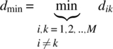
When M is large and/or the calculation of M(M−1)/2 Euclidean distances between M signal points is cumbersome, then one may replace all the Euclidean distances with the minimum Euclidean distance dmin of the signal constellation. The minimum Euclidean distance is defined as the smallest Euclidean distance between any two transmitted signal points in the constellation:
(7.69)
Replacing dik by dmin in (7.68), the average symbol error probability may be expressed as a function of the minimum Euclidean distance:
which is evidently looser than (7.68). To overcome this inconvenience, one may replace (M−1) in (7.70) by Mclosest which denotes the number of signal points closest to the signal point in the constellation, that is, the number of signal points which dominate the symbol errors.
Figure 7.16 Geometric Illustration of the Exact Symbol Error Probability and the Union Bound.
Figure 7.17 Variation of the Exact Symbol Error Probability and the Union Bounds for QPSK Signaling as a Function of Eb/N0 (dB).
7.4.2 Bit Error Versus Symbol Error
In Gray coding, the neighbouring symbols in symbol space differ in only one bit position. If there is a symbol error, then the decoder will most probably estimate nearest symbols as being sent, thus causing a single bit error. Then, the bit error probability Pb is approximated by
(7.76)
In binary coding, all symbol errors are assumed equally likely. Therefore, the Pb is related to Pe by
(7.77)
Figure 7.18 Block Diagram of a Matched‐Filter Receiver for the Signaling System Described by (7.78).
Figure 7.19 Constellation diagram and optimal decision boundaries/regions for the considered signaling scheme in Example 7.8.
References
[1] J. G. Proakis and M. Salahi, Communication Systems Engineering (2nd ed.), Prentice Hall: New Jersey, 2002.
[2] S. Haykin, Communication Systems (3rd ed.), John Wiley: New York, 1994.
[3] B. Sklar, Digital communications, Fundamentals and Applications (2nd ed.), Prentice Hall: New Jersey, 2003.
[4] A. B. Carlson, P. B. Crilly, and J. C. Rutledge, Communication Systems (4th ed.), McGraw Hill, Boston, 2002.
Problems
Consider the signal constellation shown below.
What is the dimension of this constellation?
Determine the average symbol energy in terms of E.
Express the signals in terms of the orthonormal basis functions that you choose.
Show the optimum decision regions in the signal space shown above.
Determine the error probability of the optimum receiver and compare with that of the QPSK.
Consider the quaternary signaling schemes shown below:
All the signals are equiprobable and the channel noise is white with PSD N0.
Show the optimum decision regions in these consellations.
Which constellation requires minimum energy.
Determine the error probability of the optimum receiver for these consellations.
Consider QPSK signalling defined by the constellation points
Assume that the symbols are not equally likely, and have the a priori probabilities p(s1) = p(s3) = 0.3 and p(s2) = p(s4) = 0.2.
Determine the optimum threshold levels and the decision regions that minimize error probability.
Show the decision regions in the constellation diagram.
Derive the pair‐wise error probability and determine an upper bound for the symbol error probability.
Consider the 8‐ary amplitude‐phase modulated constellation shown below where all symbols are assumed to be equally probable.
Determine the average symbol energy in terms of d and calculate peak‐to‐average power ratio.
Determine the transition probability in terms of Eb/N0 between two symbols separated by d.
Show the decision regions.
Use Gray encoding to assign three‐bits to each of the constellation points. Express the average symbol and bit error probabilities in terms of Eb/N0.
Determine the nearest neighbour union bound on the bit error probability and compare with the result you found in (d).
Consider three equi‐probable signals of average energy E. The signals are separated from each other by 120° as shown below. The channel is assumed to be AWGN with the double‐sided noise PSD N0/2.
Determine a set of orthonormal basis functions for the signal space. Write the expressions for the signals in terms of the basis functions and in vector form.
Draw the constellation diagram showing the signal vectors.
Determine the Euclidean distances between the signals and show the optimum decision boundaries.
Determine an upper bound for the average symbol error probability as a function of E/N0.
Consider the following signal set.
Determine the dimensionality and the corresponding orthonormal basis functions for this signal set.
Express the signals in terms of the orthormal basis functions.
Determine the Euclidean distance between the signal pairs and find the minimum distance.
Determine the projection of s1(t) over s3(t) and compute the angle between s1(t) and s3(t).
Consider a binary baseband communication system operating in an AWGN channel with zero mean and PSD N0/2. The received signal is ±A during each symbol duration T. The probability of transmitting +A is 0.4 and the probability of transmitting –A is 0.6. An integrate‐and‐dump filter is used for demodulation and the detector operates with a threshold level λ.
Use MAP rule to formulate the decision rule in terms of the likelihood functions and the threshold level, λ.
Determine the optimum threshold level λopt that minimizes the average error probability.
Derive an expression for the minimum average error probability.
Consider an asymmetric signal constellation with equally likely symbols:
Determine the Euclidean distances between the symbols. What is the minimum Euclidean distance?
Compute the average symbol error probability using the two bounds given by
Which pair‐wise error probability dominates the upper bound on the average symbol error probability? Explain.
Compute the upper bound when all the Euclidean distances found in (a) are assumed equal to the minimum Euclidean distance. Compare the result you found with the one determined in (b).
Consider the four basis functions {ϕ1(t), ϕ2(t), ϕ3(t), ϕ4(t)} described by the Hadamard sequences: {1111, 1010, 1100, 1001}, where the bit 0 is represented by −1V and the bit 1 by +1V.
Show that these waveforms are orthonormal
Determine the Euclidean distances between all the vector pairs.
Express the waveform x(t) as a linear combination of {ϕi(t)}, and find the coefficients, where x(t) is given by
Repeat Question 7.9 for the four basis functions {ϕ1(t), ϕ2(t), ϕ3(t), ϕ4(t)} described by {1000, 0100, 0010, 0001}.
Consider a quarternary (M = 4) phase shift keying (PSK) system, where the four symbols are located at , where E is the symbol energy. Determine the upper bound on the probability of symbol error, assuming that the probability of transmitting each symbol is the same, and compare with the exact expression for the probability of symbol error.
Given a modulation system with M = 4 and N = 2 with four equiprobable signals defined as, apart from a constant factor , s1 = (1,1), s2 = (−1,1), s3 = (−2,−1), s4 = (2,−1).
Sketch the signal space (constellation diagram)
Write down the orthonormal basis functions for this signal space.
Write down the corresponding time‐domain signals in terms of the orthonormal basis functions.
Determine the average symbol energy.
How can you assign the di‐bits to each symbol so as to minmimize the probability of bit error?
Show the optimum decision regions and explain how you obtained them.
Determine the pairwise error probabilities and the upper bound on the average signal error probability in an AWGN channel with zero mean and a variance N0/2. Explain which Euclidean distances dominate the average symbol error probability.
Find the signal most likely to have been sent if all the signals are equally likely and the observation vector is x = (0.25,−0.25).


 , where E is the symbol energy. Determine the upper bound on the probability of symbol error, assuming that the probability of transmitting each symbol is the same, and compare with the exact expression for the probability of symbol error.
 , s1 = (1,1), s2 = (−1,1), s3 = (−2,−1), s4 = (2,−1).