
Chapter 3. The Laplace Transform
What we know is not much. What we do not know is immense.
Pierre-Simon marquis de Laplace (1749–1827), French mathematician and astronomer
3.1. Introduction
The material in this chapter is very significant for the analysis of continuous-time signals and systems. The main issues discussed are:
■ Frequency domain analysis of continuous-time signals and systems—We begin the frequency domain analysis of continuous-time signals and systems using transforms. The Laplace transform, the most general of these transforms, will be followed by the Fourier transform. Both provide complementary representations of a signal to its own in the time domain, and an algebraic characterization of systems. The Laplace transform depends on a complex variable s = σ + jΩ, composed of damping σ and frequency Ω, while the Fourier transform considers only frequency Ω.
■ Damping and frequency characterization of continuous-time signals—The growth or decay of a signal—damping—as well as its repetitive nature—frequency—in the time domain are characterized in the Laplace domain by the location of the roots of the numerator and denominator, or zeros and poles, of the Laplace transform of the signal.
■ Transfer function characterization of continuous-time LTI systems—The Laplace transform provides a significant algebraic characterization of continuous-time systems: The ratio of the Laplace transform of the output to that of the input—or the transfer function of the system. It unifies the convolution integral and the differential equations system representations. The concept of transfer function is not only useful in analysis but also in design, as we will see later. The location of the poles and the zeros of the transfer function relates to the dynamic characteristics of the system.
■ Stability, and transient and steady-state responses—Certain characteristics of continuous-time systems can only be verified or understood via the Laplace transform. Such is the case of stability, and of transient and steady-state responses. This is a significant reason to study the Laplace analysis before the Fourier analysis, which deals exclusively with the frequency characterization of continuous-time signals and systems. Stability and transients are important issues in classic control theory, thus the importance of the Laplace transform in this area. The frequency characterization of signals and the frequency response of systems—provided by the Fourier transform—are significant in communications.
■ One- and two-sided Laplace transforms—Given the prevalence of causal signals (those that are zero for negative time) and of causal systems (having zero impulse responses for negative time) the Laplace transform is typically known as “one-sided,” but the “two-sided” transform also exists. The impression is that these are two different transforms, but in reality it is the Laplace transform applied to two different types of signals and systems. We will show that by separating the signal into its causal and its anti-causal components, we only need to apply the one-sided transform. Care should be exercised, however, when dealing with the inverse transform so as to get the correct signal.
■ Region of convergence and the Fourier transform—Since the Laplace transform requires integration over an infinite domain, it is necessary to consider if and where this integration converges—or the “region of convergence” in the s-plane. Now, if such a region includes the jΩ axis of the s-plane, then the Laplace transform exists for s = jΩ, and when computed there it coincides with the Fourier transform of the signal. Thus, the Fourier transform for a large class of functions can be obtained directly from their Laplace transforms—a good reason to study first the Laplace transform. In a subtle way, the Laplace transform is also connected with the Fourier series representation of periodic continuous-time signals. Such a connection reduces the computational complexity of the Fourier series by eliminating integration in cases when we can compute the Laplace transform of a period.
■ Eigenfunctions of LTI systems—LTI systems respond to complex exponentials in a very special way: The output is the exponential with its magnitude and phase changed by the response of the system at the exponent. This provides the characterization of the system by the Laplace transform, in the case of exponents of the complex frequency s, and by the Fourier representation when the exponent is jΩ. The eigenfunction concept is linked to phasors used to compute the steady-state response in circuits (see Figure 3.1).

3.2. The Two-Sided Laplace Transform
Rather than giving the definitions of the Laplace transform and its inverse, let us see how they could be obtained intuitively. As indicated before, a basic idea in characterizing signals—and their response when applied to LTI systems—is to consider them a combination of basic signals for which we can easily obtain a response. In Chapter 2, when considering the time-domain solutions, we represented the input as an infinite combination of impulses occurring at all possible times and weighted by the value of the input signal at those times. The reason we did so is because the response due to an impulse is the impulse response of the LTI system, which is fundamental in our studies. A similar approach will be followed when attempting to obtain the frequency-domain representation of signals and their responses when applied to an LTI system. In this case, the basic functions used are complex exponentials or sinusoids that depend on frequency. The concept of eigenfunction is somewhat abstract at the beginning, but after you see it applied here and in the Fourier representation later you will think of it as a way to obtain a representation analogous to the impulse representation. You will soon discover the importance of using complex exponentials, and it will then become clear that eigenfunctions are connected with phasors that greatly simplify the sinusoidal steady-state solution of circuits.
3.2.1. Eigenfunctions of LTI Systems
Consider as the input of an LTI system the complex signal
(3.1)
1German mathematician David Hilbert (1862–1943) seems to be the first to use the German word eigen to denote eigenvalues and eigenvectors in 1904. The word eigen means own or proper.
An input  , is called an eigenfunction of an LTI system with impulse response h(t) if the corresponding output of the system is

Remarks
■ You could think of H(s) as an infinite combination of complex exponentials, weighted by the impulse response h(τ). One can use a similar representation for signals.
■ Consider now the significance of applying the eigenfunction result. Suppose a signal x(t) is expressed as a sum of complex exponentials in s = σ + jΩ,
Now we are ready for the proper definition of the direct and inverse Laplace transforms of a signal or of the impulse response of a system.
The two-sided Laplace transform of a continuous-time function f(t) is
(3.2)

The inverse Laplace transform is given by
(3.3)
Remarks
■ The Laplace transform F(s) provides a representation of f(t) in the s-domain, which in turn can be converted back into the original time-domain functon in a one-to-one manner using the region of convergence. Thus,
■ If f(t) = h(t), the impulse response of an LTI system, then H(s) is called the system or transfer function of the system and it characterizes the system in the s-domain just like h(t) does in the time-domain. If f(t) is a signal, then F(s) is its Laplace transform.
■ The inverse Laplace transform inEquation (3.3)can be understood as the representation of f(t) (whether it is a signal or an impulse response) by an infinite summation of complex exponentials with weights F(s) at each. The computation of the inverse Laplace transform usingEquation (3.3)requires complex integration. Algebraic methods will be used later to find the inverse Laplace transform, thus avoiding the complex integration.
Laplace and Heaviside
The Marquis Pierre-Simon de Laplace (1749–1827) 2 and 7 was a French mathematician and astronomer. Although from humble beginnings he became royalty by his political abilities. As an astronomer, he dedicated his life to the work of applying the Newtonian law of gravitation to the entire solar system. He was considered an applied mathematician and, as a member of the Academy of Sciences, knew other great mathematicians of the time such as Legendre, Lagrange, and Fourier. Besides his work on celestial mechanics, Laplace did significant work in the theory of probability from which the Laplace transform probably comes. He felt that “the theory of probabilities is only common sense expressed in number.” Early transformations similar to Laplace's had been used by Euler and Lagrange. It was, however, Oliver Heaviside (1850–1925) who used the Laplace transform in the solution of differential equations. Heaviside, an Englishman, was a self-taught electrical engineer, mathematician, and physicist [76].
A problem in wireless communications is the so-called multipath effect on the transmitted message. Consider the channel between the transmitter and the receiver as a system like the one depicted in Figure 3.2. The sent message x(t) does not necessarily go from the transmitter to the receiver directly (line of sight) but it may take different paths, each with different length so that the signal in each path is attenuated and delayed differently. 2 At the receiver, these delayed and attenuated signals are added, causing a fading effect—given the different phases of the incoming signals their addition at the receiver results in a weak or a strong signal, thus giving the sensation of the message fading back and forth. If x(t) is the message sent from the transmitter, and the channel has N different paths with attenuation factors {αi} and corresponding delays {ti}, i = 0, …, N, use the eigenfunction property to find the system function of the channel causing the multipath effect.
2Typically, there are three effects each path can have on the sent signal: The distance the signal needs to travel (in each path this is due to reflection or refraction on buildings, structures, cars, etc.) determines how much it is attenuated and delayed (the longer the path, the more attenuated and delayed with respect to the time it was sent) and the third effect is a frequency shift—or Doppler effect—that is caused by the relative velocity between the transmitter and the receiver.
 |
| Figure 3.2 |
Solution
The output of the channel or multipath system in Figure 3.2 can be written as
(3.4)
Considering s = σ + jΩ as the variable, the response of the multipath system to x(t) = est is y(t) = x(t)H(s), so that when replacing them in Equation (3.4), we get
Let us consider the different types of functions (either continuous-time signals or the impulse responses of continuous-time systems) we might be interested in calculating Laplace transforms of.
■ Finite support functions: the function f(t) in this case is
■ Infinite support functions: In this case, f(t) is defined over an infinite support (e.g., t1 < t < t2 where either t1 or t2 are infinite, or both are infinite as long as t1 < t2).
A finite, or infinite, support function f(t) is called (see examples in Figure 3.3):
■ Casual if f(t) = 0 t < 0,
■ Anti-causal if f(t) = 0 t ≥ 0,
■ Non causal if a combination of the above.
 |
| Figure 3.3 |
In each of these cases we need to consider the region in the s-plane where the transform exists or its region of convergence (ROC). This is obtained by looking at the convergence of the transform.
For the Laplace transform of f(t) to exist we need that

3.2.2. Poles and Zeros and Region of Convergence
The region of convergence (ROC) can be obtained from the conditions for the integral in the Laplace transform to exist. The ROC is related to the poles of the transform, which is in general a complex rational function.
For a rational function  , its zeros are the values of s that make the function F(s) = 0, and its poles are the values of s that make the function F(s) → ∞. Although only finite zeros and poles are considered, infinite zeros and poles are also possible.
Typically, F(s) is rational, a ratio of two polynomials N(s) and D(s), or F(s) = N(s)/D(s), and as such its zeros are the values of s that make the numerator polynomial N(s) = 0, while the poles are the values of s that make the denominator polynomial D(s) = 0. For instance, for


Not all rational functions have poles or a finite number of zeros. Consider the Laplace transform
P(s) seems to have a pole at s = 0. Its zeros are obtained by letting es − e−s = 0, which when multiplied by es gives
Poles and ROC
The ROC consists of the values of σ such that
(3.5)
Two general comments that apply to all types of signals when finding ROCs are:
■ No poles are included in the ROC, which means that for the ROC to be that region where the Laplace transform is defined, the transform cannot become infinite at any point in it. So poles should not be present in the ROC.
■ The ROC is a plane parallel to the jΩ axis, which means that it is the damping σ that defines the ROC, not frequency Ω. This is because when we compute the absolute value of the integrand in the Laplace transform to test for convergence, we let s = σ + jΩ and the term |e−jΩt| = 1. Thus, all regions of convergence will contain −∞ < Ω < ∞.
If {σi} are the real parts of the poles of  , the region of convergence corresponding to different types of signals or impulse responses is determined from its poles as follows:
■ For a causal f(t), f(t) = 0 for t < 0, the region of convergence of its Laplace transform F(s) is a plane to the right of the poles,
■ For an anti-causal f(t), f(t) = 0 for t > 0, the region of convergence of its Laplace transform F(s) is a plane to the left of the poles,
■ For a noncausal f(t) (i.e., f(t) defined for −∞ < t < ∞), the region of convergence of its Laplace transform F(s) is the intersection of the regions of convergence corresponding to the causal component,  , and
, and  corresponding to the anti-causal component:
See Figure 3.5 for an example illustrating how the ROCs connect with the poles and the type of signal.

Indeed, the integral defining the Laplace transform is bounded for any value of σ ≠ 0. If A = max(|f(t)|), then

The Laplace transform of a
■ Finite support function (i.e., f(t) = 0 for t < t1 and t > t2, for t1 < t2) is
■ Causal function (i.e., f(t) = 0 for t < 0) is
■ Anti-causal function (i.e., f(t) = 0 for t > 0) is
■ Noncausal function (i.e., f(t) = fac(t) + fc(t) = f(t)u(−t) + f(t)u(t)) is
Although redundant, a causal function f(t)(i.e., f(t) = 0 for t < 0) is denoted as f(t)u(t). Its Laplace transform is thus

A noncausal signal f(t) is defined for all values of t (i.e., for −∞ < t < ∞). Such a signal has a causal component fc(t), which is obtained by multiplying f(t) by the unit-step function, fc(t) = f(t)u(t), and an anti-causal component fac(t), which is obtained by multiplying f(t) by u(−t), so that
(3.6)
(3.7)

3.3. The One-Sided Laplace Transform
The one-sided Laplace transform is defined as
(3.8)
Remarks
■ If f(t) is causal the multiplication by u(t) is redundant but harmless, but if f(t) is not causal the multiplication by u(t) makes f(t)u(t) causal. Notice that when f(t) is causal, the two-sided and the one-sided Laplace transforms of f(t) coincide.
■ The lower limit of the integral in the one-sided Laplace transform is set to 0− = 0 − ε, which corresponds to a value on the left side of 0 for an infinitesimal value ε. The reason for this is to make sure that an impulse function δ(t), only defined at t = 0, is included when we are computing its Laplace transform. For any other signal this limit can be taken as 0 with no effect on the transform.
■ As we will see, the advantage of the one-sided Laplace transform is that it can be used in the solution of differential equations with initial conditions. In fact, the two-sided Laplace transform by starting at t = −∞ (lower bound of the integral) ignores initial conditions at t = 0, and thus it is not useful in solving differential equations unless the initial conditions are zero.
Find the Laplace transforms of δ (t), u(t), and a pulse p(t) = u(t) − u(t − 1). Use MATLAB to verify the transforms.
Solution
Even though δ (t) is not a regular signal, its Laplace transform can be easily obtained:
The Laplace transform of u(t) can be found as

In the region of convergence, the integral is found to be
We can find the Laplace transform of signals using symbolic computations in MATLAB. For the unit-step and the delta functions, once the symbolic parameters are defined, the MATLAB function laplace computes their Laplace transforms as indicated by the following script.
%%%%%%%%%%%%%%%%%
% Example 3.2
%%%%%%%%%%%%%%%%%
syms t s
u=sym('heaviside(t)')
U=laplace(u)
% Delta function
d=sym('dirac(t)')
D=laplace(d)
giving
u=Heaviside(t)
U=1/s
d=Dirac(t)si
D=1
where U and D stand for the Laplace transforms of u and d. The naming of u(t) and δ (t) as Heaviside and Dirac functions is used in MATLAB. 3
3Oliver Heaviside (1850–1925) was an English electrical engineer who adapted the Laplace transform to the solution of differential equations (the so-called operational calculus), while Paul Dirac (1902–1984) was also an English electrical engineer, better known for his work in physics.
The pulse p(t) = u(t) − u(t − 1) is a finite support signal and so its ROC is the whole s-plane. Its Laplace transform is

Let us find and use the Laplace transform of  to obtain the Laplace transform of x(t) = cos(Ω0t + θ)u(t). Consider the special cases for θ = 0 and θ = −π/2. Determine the ROCs. Use MATLAB to plot the signals and the corresponding poles/zeros when Ω0 = 2 and θ = 0 and π/4.
Solution
The Laplace transform of the complex causal signal  is found to be


Now if we let θ = 0, −π/2 in the above equation we have the following Laplace transforms:

Use MATLAB symbolic computation to find the Laplace transform of a real exponential, x(t) = e−tu(t), and of x(t) modulated by a cosine or y(t) = e−t cos(10t)u(t). Plot the signals and the poles and zeros of their Laplace transforms.
Solution
The following script is used. The MATLAB function laplace is used for the computation of the Laplace transform and the function ezplot allows us to do the plotting. For the plotting of the poles and zeros we use our function splane. When you run the script you obtain the Laplace transforms
%%%%%%%%%%%%%%%%%
% Example 3.4
%%%%%%%%%%%%%%%%%
syms t
x=exp (-t);
y=x*cos(10*t);
X=laplace(x)
Y=laplace(y)
% plotting of signals and poles/zeros
figure(1)
subplot(221)
ezplot(x,[0,5]);grid
axis([0 5 0 1.1]);title('x(t)=exp(-t)u(t)')
numx=[0 1];denx=[1 1];
subplot(222)
splane(numx,denx)
subplot(223)
ezplot(y,[-1,5]);grid
axis([0 5 -1.1 1.1]);title('y(t)=cos(10t)exp(-t)u(t)')
numy=[0 1 1];deny=[1 2 101];
subplot(224)
splane(numy,deny)
The results are shown in Figure 3.7.

In statistical signal processing, the autocorrelation function c(τ) of a random signal describes the correlation that exists between the random signal x(t) and shifted versions of it, x(t + τ) and x(t − τ) for shifts −∞ < τ < ∞. Clearly, c(τ) is two-sided (i.e., nonzero for both positive and negative values of τ) and symmetric. Its two-sided Laplace transform is related to the power spectrum of the signal x(t). Let c(t) = e−a|t|, where a > 0 (we replaced the τ variable for t for convenience). Find its Laplace transform. Determine if it would be possible to compute |C(Ω)|2, which is called the power spectrum of the random signal x(t).
Solution
The autocorrelation can be expressed as

We thus have that


Consider a noncausal LTI system with impulse response

Solution
As from before, the Laplace transform of the causal component, hc(t), is
Thus, the system function is
Compute the Laplace transform of the ramp function r(t) = tu(t) and use it to find the Laplace of a triangular pulse Λ(t) = r(t + 1) − 2r(t) + r(t − 1).
Solution
Notice that although the ramp is an ever-increasing function of t, we still can obtain its Laplace transform


In particular, when k = 0 there are two zeros at 0, which cancel the two poles at 0 resulting from the denominator s2. Thus, Λ(s) has an infinite number of zeros but no poles given this pole-zero cancellation (see Figure 3.9). Therefore, Λ(s) has the whole s-plane as its region of convergence, and can be calculated at s = jΩ.

We will consider next the basic properties of the one-sided Laplace transform—many of these properties will be encountered in the Fourier analysis, presented in a slightly different form, given the connection between the Laplace and the Fourier transforms. Something to observe is the duality that exists between the time and the frequency domains. The time and the frequency domain representations of continuous-time signals and systems are complementary—that is, certain characteristics of the signal or the system can be seen better in one domain than in the other. In the following, we consider the properties of the Laplace transform of signals but they equally apply to the impulse response of a system.
3.3.1. Linearity
For signals f(t) and g(t), with Laplace transforms F(s) and G(s), and constants a and b, we have the Laplace transform is linear:
The linearity of the Laplace transform is easily verified using integration properties:

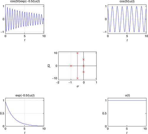
We will use the linearity property to illustrate the significance of the location of the poles of the Laplace transform of causal signals. As seen before, the Laplace transform of an exponential signal f(t) = Ae−atu(t) where a in general can be a complex number is
The Laplace transform F(s) = 1/(s + a) of f(t) = e−atu(t), for any real value of a, has a pole on the real axis σ of the s-plane, and we have the following three cases:
■ For a = 0, the pole at the origin s = 0 corresponds to the signal f(t) = u(t), which is constant for t ≥ 0(i.e., it does not decay).
■ For a > 0, the signal is f(t) = e−atu(t), a decaying exponential, and the pole s = −a of F(s) is in the real axis σ of the left-hand s-plane. As the pole is moved away from the origin toward the left, the faster the exponential decays, and as it moves toward the origin, the slower the exponential decays.
■ For a < 0, the pole s = −a is on the real axis σ of the right-hand s-plane, and corresponds to a growing exponential. As the pole moves to the right the exponential grows faster, and as it is moved toward the origin it grows at a slower rate—clearly this signal is not useful, as it grows continuously.
The conclusion is that the σ axis of the Laplace plane corresponds to damping. A single pole on this axis and in the left-hand s-plane corresponds to a decaying exponential, and a single pole on this axis and in the right-hand s-plane corresponds to a growing exponential.
Suppose then we consider
(3.9)
The conclusion is that the Laplace transform of a sinusoid has a pair of poles on the jΩ axis. For these poles to correspond to a real-valued signal they should be complex conjugate pairs, requiring negative as well as positive values of the frequency. Furthermore, when these poles are moved away from the origin of the jΩ axis, the frequency increases, and the frequency decreases whenever the poles are moved toward the origin.
Finally, consider the case of a signal d(t) = Ae−αt cos(Ω0t)u(t) or a causal sinusoid multiplied (or modulated) by e−αt. According to Euler's identity,
(3.10)
The conclusion is that the location of the poles (and to some degree the zeros), as indicated in the previous two cases, determines the characteristics of the signal. Signals are characterized by their damping and frequency and as such can be described by the poles of its Laplace transform.
If we were to add the different signals considered above, then the Laplace transform of the resulting signal would be the sum of the Laplace transform of each of the signals and the poles would be the aggregation of the poles from each. This observation will be important when finding the inverse Laplace transform, then we would like to do the opposite: To isolate poles or pairs of poles (when they are complex conjugate) and associate with each a general form of the signal with parameters that are found by using the zeros and the other poles of the transform. Figure 3.10 provides an example illustrating the importance of the location of the poles, and the significance of the σ and jΩ axes.
3.3.2. Differentiation
For a signal f(t) with Laplace transform F(s) the one-sided Laplace transform of its first-and second-order derivatives are
(3.12)
(3.13)
The Laplace transform of the derivative of a causal signal is

Remarks
■ The derivative property for a signal x(t) defined for all t is


■ Application of the linearity and the derivative properties of the Laplace transform makes solving differential equations an algebraic problem.
Find the impulse response of an RL circuit in series with a voltage source vs(t) (see Figure 3.11). The current i(t) is the output and the input is the voltage source vs(t).

Solution
To find the impulse response of the RL circuit we let vs(t) = δ (t) and set the initial current in the inductor to zero. According to Kirchhoff's voltage law,
Letting vs(t) = δ (t) and computing the Laplace transform of the above equation (using the linearity and the derivative properties of the transform and remembering the initial condition is zero), we obtain the following equation in the s-domain:
In this example we consider the duality between the time and the Laplace domains. The differentiation property indicates that computing the derivative of a function in the time domain corresponds to multiplying by s the Laplace transform of the function (assuming initial conditions are zero). We will illustrate in this example the dual of this—that is, when we differentiate a function in the s-domain its effect in the time domain is to multiply by −t. Consider the connection between δ (t), u(t), and r(t) (i.e., the unit impulse, the unit step, and the ramp, respectively), and relate it to the indicated duality. Explain how this property connects with the existence of multiple poles, real and complex, in general.
Solution
The relation between the signals δ (t), u(t), and r(t) is seen from

The above results can be explained by looking for a dual of the derivative property. Multiplying by −t the signal x(t) corresponds to differentiating X(s) with respect to s. Indeed for an integer N > 1,

What about multiple real (different from zero) and multiple complex poles? What are the corresponding inverse Laplace transforms? The inverse Laplace transform of
Obtain from the Laplace transform of x(t) = cos(Ω0t)u(t) the Laplace transform of sin(t)u(t) using the derivative property.


Notice that whenever the signal is discontinuous at t = 0, as in the case of x(t) = cos(Ω0t)u(t), its derivative will include a δ (t) signal due to the discontinuity. On the other hand, whenever the signal is continuous at t = 0, for instance y(t) = sin(Ω0t)u(t), its derivative does not contain δ (t) signals. In fact,

3.3.3. Integration
The Laplace transform of the integral of a causal signal y(t) is given by
(3.14)

This property can be shown by using the derivative property. Call the integral


Suppose that

Solution
Applying the integration property gives
3.3.4. Time Shifting
If the Laplace transform of f(t)u(t) is F(s), the Laplace transform of the time-shifted signal f(t − τ)u(t − τ) is
(3.15)
This indicates that when we delay (advance) the signal to get f(t − τ)u(t − τ) (f(t + τ)u(t + τ)) its corresponding Laplace transform is F(s) multiplied by e−τs (eτs). This property is easily shown by a change of variable when computing the Laplace transform of the shifted signals.
Suppose we wish to find the Laplace transform of the causal sequence of pulses x(t) shown in Figure 3.12. Let x1(t) denote the first pulse (i.e., for 0 ≤ t < 1).

Solution
We have for t ≥ 0,

The poles of X(s) are the poles of X1(s) and the roots of 1 − e−s = 0 (the s values such that e−s = 1, or sk = ±j2π k for any integer k ≥ 0). Thus, there is an infinite number of poles for X(s), and the partial fraction expansion method that uses poles to invert Laplace transforms, presented later, will not be useful. The reason this example is presented here, ahead of the inverse Laplace, is to illustrate that when we are finding the inverse of this type of Laplace function we need to consider the time-shift property, otherwise we would need to consider an infinite partial fraction expansion.
Consider the causal full-wave rectified signal shown in Figure 3.13. Find its Laplace transform.

Solution
The first period of the full-wave rectified signal can be expressed as
3.3.5. Convolution Integral
Because this is the most important property of the Laplace transform we provide a more extensive coverage later, after considering the inverse Laplace transform.
If the input of an LTI system is the causal signal x(t) and the impulse response of the system is h(t), then the output y(t) can be written as

The system function or transfer function  , the Laplace transform of the impulse response h(t) of an LTI system, can be expressed as the ratio
(3.17)
3.4. Inverse Laplace Transform
Inverting the Laplace transform consists in finding a function (either a signal or an impulse response of a system) that has the given transform with the given region of convergence. We will consider three cases:
■ Inverse of one-sided Laplace transforms giving causal functions.
■ Inverse of Laplace transforms with exponentials.
■ Inverse of two-sided Laplace transforms giving anti-causal or noncausal functions.
The given function X(s) we wish to invert can be the Laplace transform of a signal or a transfer function—that is, the Laplace transform of an impulse response.
3.4.1. Inverse of One-Sided Laplace Transforms
When we consider a causal function x(t), the region of convergence of X(s) is of the form
The most common inverse Laplace method is the so-called partial fraction expansion, which consists in expanding the given function in s into a sum of components of which the inverse Laplace transforms can be found in a table of Laplace transform pairs. Assume the signal we wish to find has a rational Laplace transform—that is,
(3.18)
(3.19)
(3.20)
Remarks
■ Things to remember before performing the inversion are:
■ The poles of X(s) provide the basic characteristics of the signal x(t).
■ If N(s) and D(s) are polynomials in s with real coefficients, then the zeros and poles of X(s) are real and/or complex conjugate pairs, and can be simple or multiple.
■ In the inverse, u(t) should be included since the result of the inverse is causal—the function u(t) is an integral part of the inverse.
■ The basic idea of the partial expansion is to decompose proper rational functions into a sum of rational components of which the inverse transform can be found directly in tables.Table 3.1displays common one-sided Laplace transform pairs, whileTable 3.2provides properties of the one-sided Laplace transform.
We will consider now how to obtain a partial fraction expansion when the poles are real, simple and multiple, and in complex conjugate pairs, simple and multiple.
Simple Real Poles
According to Laplace transform tables the time function corresponding to Ak/(s − pk) is  , thus the form of the inverse x(t). To find the coefficients of the expansion, say Aj, we multiply both sides of the Equation (3.22) by the corresponding denominator (s − pj) so that

Consider the proper rational function
Solution
The partial fraction expansion is
To check that the solution is correct one could use the initial or the final value theorems shown in Table 3.2. According to the initial value theorem, x(0) = 3 should coincide with


Remarks
The coefficients A1and A2can be found using other methods. For instance,
■ We can compute
(3.23)
■ We cross-multiply the partial expansion given byEquation (3.23)to get
Simple Complex Conjugate Poles
The partial fraction expansion of a proper rational function
(3.24)

(3.25)
Because the numerator and the denominator polynomials of X(s) have real coefficients, the zeros and poles whenever complex appear as complex conjugate pairs. One could thus think of the case of a pair of complex conjugate poles as similar to the case of two simple real poles presented above. Notice that the numerator N(s) must be a first-order polynomial for X(s) to be proper rational. The poles of X(s), s1,2 = −α ± jΩ0, indicate that the signal x(t) will have an exponential e−αt, given that the real part of the poles is −α, multiplied by a sinusoid of frequency Ω0, given that the imaginary parts of the poles are ±Ω0. We have the expansion


Remarks
■ An equivalent partial fraction expansion consists in expressing the numerator N(s) of X(s), for some constants a and b, as N(s) = a + b(s + α), a first-order polynomial, so that

■ When α = 0 the above indicates that the inverse Laplace transform of
■ When the frequency Ω0 = 0, we get that the inverse Laplace transform of

Consider the Laplace function
Solution
The poles are at  , so that we expect that x(t) is a decaying exponential with a damping factor of −1 (the real part of the poles) multiplied by a causal cosine of frequency
  . The partial fraction expansion is of the form


We use the MATLAB function ilaplace to compute symbolically the inverse Laplace transform and plot the response using ezplot, as shown in the following script.
%%%%%%%%%%%%%%%%%
% Example 3.15
%%%%%%%%%%%%%%%%%
clear all; clf
syms s t w
num=[0 2 3]; den=[1 2 4]; % coefficients of numerator and denominator
subplot(121)
splane(num,den) % plotting poles and zeros
disp(‘>>>>> Inverse Laplace <<<<<’)
x = ilaplace((2*s + 3)/(s^2 + 2*s + 4)); % inverse Laplace transform
ezplot(x,[0,12]); title('x(t)')
axis([0 12 -0.5 2.5]); grid
The results are shown in Figure 3.14.

Double Real Poles
When we have double real poles we need to express the numerator N(s) as a first-order polynomial, just as in the case of a pair of complex conjugate poles. The values of a and b can be computed in different ways, as we illustrate in the following examples.
Typically, the Laplace transforms appear as combinations of the different terms we have considered, for instance a combination of first- and second-order poles gives
Solution
The partial fraction expansion is
The initial value x(0) = 0 coincides with


Remarks
■ Following the above development, when the poles are complex conjugate and double the procedure for the double poles is repeated. Thus, the partial expansion is given as
(3.28)

■ The partial fraction expansion for second- and higher-order poles should be done with MATLAB.
In this example we use MATLAB to find the inverse Laplace transform of more complicated functions than the ones considered before. In particular, we want to illustrate some of the additional information that our function pfeLaplace gives. Consider the Laplace transform
Solution
function pfeLaplace(num,den)
%
disp(‘>>>>> Zeros <<<<<’)
z = roots(num)
[r,p,k]=residue(num,den);
disp(‘>>>>> Poles <<<<<’)
p
disp(‘>>>>> Residues <<<<<’)
r
splane(num,den)
The function pfeLaplace uses the MATLAB function roots to find the zeros of X(s) defined by the coefficients of its numerator and denominator given in descending order of s. For the partial fraction expansion, pfeLaplace uses the MATLAB function residue, which finds coefficients of the expansion as well as the poles of X(s). (The residue r(i) in the vector r corresponds to the expansion term for the pole p(i); for instance, the residue r(1) = 8 corresponds to the expansion term corresponding to the pole p(1) = −3.) The symbolic function ilaplace is then used to find the inverse x(t); as input to ilaplace the function X(s) is described in a symbolic way. The MATLAB function ezplot is used for the plotting of the symbolic computations.
The analytic results are shown in the following, and the plot of x(t) is given in Figure 3.16.
 |
| Figure 3.16 |
>>>>> Zeros <<<<<
z=-1.6667
1.0000
>>>>> Poles <<<<<
p=-3.0000
-2.0000
-1.0000
>>>>> Residues <<<<<
r=8.0000
-3.0000
-2.0000
>>>>> Inverse Laplace <<<<<
x=8*exp(-3*t)-3*exp(-2*t)-2*exp(-t)
3.4.2. Inverse of Functions Containing e−ρs Terms
When X(s) has exponentials e−ρs in the numerator or denominator, ignore these terms and perform partial fraction expansion on the rest, and at the end consider the exponentials to get the correct time shifting. In particular, when


The time-shifting property of Laplace makes it possible for the numerator N(s) or the denominator D(s) to have e−σs terms. The procedure for inverting such functions is to initially ignore these terms and do the partial fraction expansion on the rest and at the end consider them to do the necessary time shifting. For instance, the inverse of


3.4.3. Inverse of Two-Sided Laplace Transforms
When finding the inverse of a two-sided Laplace transform we need to pay close attention to the region of convergence and to the location of the poles with respect to the jΩ axis. Three regions of convergence are possible:
■ A plane to the right of all the poles, which corresponds to a causal signal.
■ A plane to the left of all poles, which corresponds to an anti-causal signal.
■ A region that is in between poles on the right and poles on the left (no poles included in it), which corresponds to a two-sided signal.
If the jΩ axis is included in the region of convergence, bounded-input bounded-output (BIBO) stability of the system, or absolute integrability of the impulse response of the system, is guaranteed. Furthermore, the system with that region of convergence would have a frequency response, and the signal a Fourier transform. The inverses of the causal and the anti-causal components are obtained using the one-sided Laplace transform.
Find the inverse Laplace transform of
Solution
The ROC  is equivalent to {(σ, Ω): −2 < σ < 2, −∞ < Ω <∞}. The partial fraction expansion is
Consider the transfer function
Solution
The following are the different possible impulse responses:
■ If ROC:  , the impulse response
■ If ROC:  , the impulse response corresponding to H(s) with this region of convergence is noncausal, but the system is stable. The impulse response would be
■ If ROC:  , the impulse response in this case would be anti-causal, and the system is unstable (please verify it), as the impulse response is
Two very important generalizations of the results in this example are:
■ If the system is BIBO stable and causal, then the region of convergence includes the jΩ axis so that the frequency response H(jΩ) exists, and all the poles of H(s) are in the open left-hand s-plane (the jΩ axis is not included).
3.5. Analysis of LTI Systems
Dynamic linear time-invariant systems are typically represented by differential equations. Using the derivative property of the one-sided Laplace transform (allowing the inclusion of initial conditions) and the inverse transformation, differential equations are changed into easier-to-solve algebraic equations. The convolution integral is not only a valid alternate representation for systems represented by differential equations, but for other systems. The Laplace transform provides a very efficient computational method for the convolution integral. More important, the convolution property of the Laplace transform introduces the concept of transfer function, a very efficient representation of LTI systems whether they are represented by differential equations or not. In Chapter 6, we will present applications of the material in this section to classic control theory.
3.5.1. LTI Systems Represented by Ordinary Differential Equations
Two ways to characterize the response of a causal and stable LTI system are:
■ Zero-state and zero-input responses, which have to do with the effect of the input and the initial conditions of the system.
■ Transient and steady-state responses, which have to do with close and faraway behavior of the response.
The complete response y(t) of a system represented by an Nth-order linear differential equation with constant coefficients,
(3.29)
(3.30)
(3.31)

The notation y(k)(t) and  indicates the kth and the
  th derivatives of y(t) and of x(t), respectively (it is to be understood that y(0)(t) = y(t) and likewise x(0)(t) = x(t) in this notation). The assumption N > M avoids the presence of δ (t) and its derivatives in the solution, which are realistically not possible. To obtain the complete response y(t) we compute the Laplace transform of Equation (3.29):

(3.32)

Zero-State and Zero-Input Responses
Despite the fact that linear differential equations, with constant coefficients, do not represent linear systems unless the initial conditions are zero and the input is causal, linear system theory is based on these representations with initial conditions. Typically, the input is causal so it is the initial conditions not always being zero that causes problems. This can be remedied by a different way of thinking about the initial conditions. In fact, one can think of the input x(t) and the initial conditions as two different inputs to the system, and apply superposition to find the responses to these two different inputs. This defines two responses. One is due completely to the input, with zero initial conditions, called the zero-state solution. The other component of the complete response is due exclusively to the initial conditions, assuming that the input is zero, and is called the zero-input solution.
Remarks
■ It is important to recognize that to compute the transfer function of the system
■ If there is no pole-zero cancellation, both H(s) and H1(s) have the same poles, as both have A(s) as denominator, and as such h(t) and h1(t) might be similar.
Transient and Steady-State Responses
Whenever the input of a causal and stable system has poles in the closed left-hand s-plane, poles in the jΩ-axis being simple, the complete response will be bounded. Moreover, whether the response exists as t → ∞ can then be determined without using the inverse Laplace transform.
The complete response y(t) of an LTI system is made up of transient and steady-state components. The transient response can be thought of as the system's reaction to the initial inertia after applying the input, while the steady-state response is how the system reacts to the input away from the initial time when the input starts.
In fact, for any real pole s = −α, α > 0, of multiplicity m ≥ 1, we have that

Simple complex conjugate poles and a simple real pole at the origin of the s-plane cause a steady-state response. Indeed, if the pole of Y(s) is s = 0 we know that its inverse transform is of the form Au(t), and if the poles are complex conjugates ±jΩ0 the corresponding inverse transform is a sinusoid—neither of which is transient. However, multiple poles on the jΩ-axis, or any poles in the right-hand s-plane will give inverses that grow as t → ∞. This statement is clear for the poles in the right-hand s-plane. For double- or higher-order poles in the jΩ axis their inverse transform is of the form
In summary, when solving differential equations—with or without initial conditions—we have
■ The steady-state component of the complete solution is given by the inverse Laplace transforms of the partial fraction expansion terms of Y(s) that have simple poles (real or complex conjugate pairs) in the jΩ-axis.
■ The transient response is given by the inverse transform of the partial fraction expansion terms with poles in the left-hand s-plane, independent of whether the poles are simple or multiple, real or complex.
■ Multiple poles in the jΩ axis and poles in the right-hand s-plane give terms that will increase as t increases.
Consider a second-order (N = 2) differential equation,
Solution
If the initial conditions are zero, computing the two- or one-sided Laplace transform of the two sides of this equation, after letting  and
and  , and using the derivative property of Laplace, we get
In a similar form we obtain the unit-step response s(t), by letting x(t) = u(t) and the initial conditions be zero. Calling  , since X(s) = 1/s, we obtain
The steady state of s(t) is 0.5 as the two exponentials go to zero. Interestingly, the relation sS(s) = H(s) indicates that by computing the derivative of s(t) we obtain h(t). Indeed,

Remarks
■ Because the existence of the steady-state response depends on the poles of Y(s) it is possible for an unstable causal system (recall that for such a system BIBO stability requires all the poles of the system transfer function be in the open, left-hand s-plane) to have a steady-state response. It all depends on the input. Consider, for instance, an unstable system with H(s) = 1/(s(s + 1)), being unstable due to the pole ats = 0; if the system input is x1(t) = u(t) so that X1(s) = 1/s, then Y1(s) = 1/(s2(s + 1)). There will be no steady state because of the double pole s = 0. On the other hand, X2(s) = s/(s + 2)2will give
■ The steady-state response is the response of the system away from t = 0, and it can be found by letting t → ∞ (even though the steady state can be reached at finite times, depending on how fast the transient goes to zero). InExample 3.22, the steady-state response of h(t) = (e−t − e−2t)u(t) is zero, while for s(t) = 0.5u(t) − e−tu(t) + 0.5e−2tu(t) it is 0.5. The transient responses are then h(t) − 0 = h(t) and s(t) − 0.5u(t) = −e−tu(t) + 0.5e−2tu(t). These transients eventually disappear.
■ The relation found between the impulse response h(t) and the unit-step response s(t) can be extended to more cases by the definition of the transfer function—that is, H(s) = Y(s)/X(s) so that the response Y(s) is connected with H(s) by Y(s) = H(s)X(s), giving the relation between y(t) and h(t). For instance, if x(t) = δ (t), then Y(s) = H(s) × 1, with inverse the impulse response. If x(t) = u(t), then Y(s) = H(s)/s is S(s), the Laplace transform of the unit-step response, and so h(t) = ds(t)/dt. And if x(t) = r(t), then Y(s) = H(s)/s2 is ρ(s), the Laplace transform of the ramp response, and so h(t) = d2ρ(t)/dt2 = ds(t)/dt.
Consider again the second-order differential equation in the previous example,
Solution
The Laplace transform of the differential equation gives


(3.36)
According to Equation (3.36), the complete solution y(t) is composed of the zero-state response, due to the input only, and the response due to the initial conditions only or the zero-input response. Thus, the system considers two different inputs: One that is x(t) = u(t) and the other the initial conditions.
If we are able to find the transfer function H(s) = Y(s)/X(s) its inverse Laplace transform would be h(t). However that is not possible when the initial conditions are nonzero. As shown above, in the case of nonzero initial conditions, we get that the Laplace transform is
Consider an analog averager represented by
(3.37)

3.5.2. Computation of the Convolution Integral
From the point of view of signal processing, the convolution property is the most important application of the Laplace transform to systems. The computation of the convolution integral is difficult even for simple signals. In Chapter 2 we showed how to obtain the convolution integral analytically as well as graphically. As we will see in this section, it is not only that the convolution property of the Laplace transform gives an efficient solution to the computation of the convolution integral, but that it introduces an important representation of LTI systems, namely the transfer function of the system. A system, like signals, is thus represented by the poles and zeros of the transfer function. But it is not only the pole-zero characterization of the system that can be obtained from the transfer function. The system's impulse response is uniquely obtained from the poles and zeros of the transfer function and the corresponding region of convergence. The way the system responds to different frequencies will be also given by the transfer function. Stability and causality of the system can be equally related to the transfer function. Design of filters depends on the transfer function.
The Laplace transform of the convolution y(t) = [x ∗ h](t) is given by the product
(3.38)
(3.39)
Use the Laplace transform to find the convolution y(t) = [x ∗ h](t) when
(1) the input is x(t) = u(t) and the impulse response is a pulse h(t) = u(t) − u(t − 1), and
(2) the input and the impulse response of the system are x(t) = h(t) = u(t) − u(t − 1).
Solution
■ The Laplace transforms are  and
and  , so that
■ In the second case,  , so that
To illustrate the significance of the Laplace approach in computing the output of an LTI system by means of the convolution integral, consider an RLC circuit in series with input a voltage source x(t) and as output the voltage y(t) across the capacitor (see Figure 3.17). Find its impulse response h(t) and its unit-step response s(t). Let LC = 1 and R/L = 2.
 |
| Figure 3.17 |
Solution
The RLC circuit is represented by a second-order differential equation given that the inductor and the capacitor are capable of storing energy and their initial conditions are not dependent on each other. To obtain the differential equation we apply Kirchhoff's voltage law (KVL)


(3.40)

In the Laplace domain, the above can be easily computed as follows. From the transfer function, we have that
Consider the positive feedback system created by a microphone close to a set of speakers that are putting out an amplified acoustic signal (see Figure 3.18), which we considered in Example 2.18 in Chapter 2. Find the impulse response of the system using the Laplace transform, and use it to express the output in terms of a convolution. Determine the transfer function and show that the system is not BIBO stable. For simplicity, let β = 1, τ = 1, and x(t) = u(t). Connect the location of the poles of the transfer function with the unstable behavior of the system.

Solution
As we indicated in Example 2.18 in Chapter 2, the impulse response of a feedback system cannot be explicitly obtained in the time domain, but it can be done using the Laplace transform. The input–output equation for the positive feedback is

For this system to be BIBO stable, the impulse response h(t) must be absolutely integrable, which is not the case for this system. Indeed,
3.6. What have We Accomplished? Where Do We Go from Here?
In this chapter you have learned the significance of the Laplace transform in the representation of signals as well as of systems. The Laplace transform provides a complementary representation to the time representation of a signal, so that damping and frequency, poles and zeros, together with regions of convergence, conform a new domain for signals. But it is more than that—you will see that these concepts will apply for the rest of this part of the book. When discussing the Fourier analysis of signals and systems we will come back to the Laplace domain for computational tools and for interpretation. The solution of differential equations and the different types of responses are obtained algebraically with the Laplace transform. Likewise, the Laplace transform provides a simple and yet very significant solution to the convolution integral. It also provides the concept of transfer function, which will be fundamental in analysis and synthesis of linear time-invariant systems.
The common thread of the Laplace and the Fourier transforms is the eigenfunction property of LTI systems. You will see that understanding this property will provide you with the needed insight into the Fourier analysis, which we will cover in the next two chapters.
Generic Signal Representation and the Laplace Transform
 Considering the integral an infinite sum of terms x(τ)δ (t − τ) (think of x(τ) as a constant, as it is not a function of time t), find the Laplace transform of each of these terms and use the linearity property to find
  . Are you surprised at this result?
The generic representation of a signal x(t) in terms of impulses is
Impulses and the Laplace Transform

Given
(a) Find the Laplace transform X(s) of x(t) and determine its region of convergence.
(b) Plot x(t).
(c) The function X(s) is complex. Let s = σ + jΩ and carefully obtain the magnitude |X(σ + jΩ)| and the phase  .
.
Sinusoids and the Laplace Transform
Consider the following cases involving sinusoids:
(a) Find the Laplace transform of y(t) = sin(2πt)u(t) − sin(2π(t − 1))u(t − 1)) and its region of convergence. Carefully plot y(t). Determine the region of convergence of Y(s).
(b) A very smooth pulse, called the raised cosine, x(t) is obtained as
(c) Indicate three possible approaches to finding the Laplace transform of cos2(t)u(t). Use two of these approaches to find the Laplace transform.
Unit-Step Signals and the Laplace Transform
Find the Laplace transform of the reflection of the unit-step signal (i.e., u(−t)) and its region of convergence. Then use the result together with the Laplace transform of u(t) to see if you can obtain the Laplace transform of a constant or u(t) + u(−t) (assume u(0) = 0.5 so there is no discontinuity at t = 0).
Laplace Transform of Noncausal Signal
 Carefully plot it, and find its Laplace transform X(s) by separating x(t) into a causal signal and an anti-causal signal, xc(t) and xac(t), respectively, and plot them separately. Find the ROC of X(s), Xc(s), and Xac(s).
Consider the noncausal signal
Transfer Function and Differential Equation

The transfer function of a causal LTI system is
(a) Find the differential equation that relates the input x(t) and the output y(t) of the system.
(b) Suppose we would like the output y(t) to be identically zero for t greater or equal to zero. If we let x(t) = δ (t), what would the initial conditions be equal to?
Transfer Function
 If the Laplace transform of the output is given by
 determine the transfer function of the system.
The input to an LTI system is
Inverse Laplace Transform—MATLAB
 which is not proper, determine the amplitude of the δ (t) and dδ(t)/dt terms in the inverse signal x(t).
 should give a response of the form
 Find the values of A, B, and C. Use the MATLAB function ilaplace to get the inverse.
Consider the following inverse Laplace transform problems for a causal signal x(t):
(a) Given the Laplace transform
(b) Find the inverse Laplace transform of
(c) The inverse Laplace transform of
Steady State and Transient
 corresponding to a causal signal x(t), determine its steady-state solution. What is the value of x(0)? Show how to obtain this value without computing the inverse Laplace transform.
 What would be the steady-state response yss(t)?
 How would you determine if there is a steady state or not? Explain.
 Determine the steady-state and the transient responses corresponding to Y(s).
Consider the following cases where we want to determine either the steady state, transient, or both.
(a) Without computing the inverse of the Laplace transform
(b) The Laplace transform of the output of an LTI system is
(c) The Laplace transform of the output of an LTI system is
(d) The Laplace transform of the output of an LTI system is
Inverse Laplace Transformation—MATLAB
Consider the following inverse Laplace problems using MATLAB for causal signal x(t):


Convolution Integral
Consider the following problems related to the convolution integral:
(a) The impulse response of an LTI system is h(t) = e−2tu(t) and the system input is a pulse x(t) = u(t) − u(t − 3). Find the output of the system y(t) by means of the convolution integral graphically and by means of the Laplace transform.
(b) It is known that the impulse response of an analog averager is h(t) = u(t) − u(t − 1). Consider the input to the averager x(t) = u(t) − u(t − 1), and determine graphically as well as by means of the Laplace transform the corresponding output of the averager y(t) = [h ∗ x](t). Is y(t) smoother than the input signal x(t)? Provide an argument for your answer.
(c) Suppose we cascade three analog averagers each with the same impulse response h(t) = u(t) − u(t − 1). Determine the transfer function of this system. If the duration of the support of the input to the first averager is M sec, what would be the duration of the support of the output of the third averager?
Deconvolution
 What is the input x(t)?
In convolution problems the impulse response h(t) of the system and the input x(t) are given and one is interested in finding the output of the system y(t). The so-called “deconvolution” problem consists in giving two of x(t), h(t), and y(t) to find the other. For instance, given the output y(t) and the impulse response h(t) of the system, one wants to find the input. Consider the following cases:
(a) Suppose the impulse response of the system is h(t) = e−t cos(t)u(t) and the output has a Laplace transform
(b) The output of an LTI system is y(t) = r(t) − 2r(t − 1) + r(t − 2), where r(t) is the ramp signal. Determine the impulse response of the system if it is known that the input is x(t) = u(t) − u(t − 1).
Application of Superposition
 Find the unit-step response s(t) of the system, and then use it to find the response due to the following inputs:
 Express the responses yi(t) due to xi(t) for i = 1, …, 4 in terms of the unit-step response s(t).
One of the advantages of LTI systems is the superposition property. Suppose that the transfer function of a LTI system is
Properties of the Laplace Transform
Consider computing the Laplace transform of a pulse

(a) Use the integral formula to find P(s), the Laplace transform of p(t). Determine the region of convergence of P(s).
(b) Represent p(t) in terms of the unit-step function and use its Laplace transform and the time-shift property to find P(s). Find the poles and zeros of P(s) to verify the region of convergence obtained above.
Frequency-Shift Property
Duality occurs between time and frequency shifts. As shown, if  , then
  . The dual of this would be
  , which we call the frequency-shift property.
(a) Use the integral formula for the Laplace transform to show the frequency-shift property.
(b) Use the above frequency-shift property to find  (represent the cosine using Euler's identity). Find and plot the poles and zeros of X(s).
(c) Recall the definition of the hyperbolic cosine,  , and find the Laplace transform Y(s) of y(t) = cosh(Ω0t)u(t). Find and plot the poles and zeros of Y(s). Explain the relation of the poles of X(s) and Y(s) by connecting x(t) with y(t).
Poles and Zeros
 and the input is the above signal x(t), compute the output z(t).
Consider the pulse x(t) = u(t) − u(t − 1).
(a) Find the zeros and poles of X(s) and plot them.
(b) Suppose x(t) is the input of an LTI system with a transfer function H(s) = 1/(s2 + 4π2). Find and plot the poles and zeros of  where y(t) is the output of the system.
(c) If the transfer function of the LTI system is
Poles and Zeros—MATLAB

 From the location of the poles, obtain a general form for x(t). Use MATLAB to find x(t) and plot it. How well did you guess the answer?
The poles corresponding to the Laplace transform X(s) of a signal x(t) are
(a) Within some constants, give a general form of the signal x(t).
(b) Let
Solving Differential Equations—MATLAB
One of the uses of the Laplace transform is the solution of differential equations.
(a) Suppose you are given the differential equation that represents an LTI system,
(b) If y(1)(0) = 1 and y(0) = 1 are the initial conditions for the above differential equation, find Y(s). If the input to the system is doubled—that is, the input is 2x(t) with Laplace transform 2X(s)—is Y(s) doubled so that its inverse Laplace transform y(t) is doubled? Is the system linear?
(c) Use MATLAB to find the poles and zeros and the solutions of the differential equation when the input is u(t) and 2u(t) with the initial conditions given above. Compare the solutions and verify your response in (b).
Differential Equation, Initial Conditions, and Impulse Response—MATLAB

The following function  is obtained applying the Laplace transform to a differential equation representing a system with nonzero initial conditions and input x(t), with Laplace transform X(s):
(a) Find the differential equation in y(t) and x(t) representing the system.
(b) Find the initial conditions y′(0) and y(0).
(c) Use MATLAB to determine the impulse response h(t) of this system. Find the poles of the transfer function H(s) and determine if the system is BIBO stable.
Different Responses—MATLAB
Let  be the Laplace transform of the solution of a second-order differential equation representing a system with input x(t) and some initial conditions,
(a) Find the zero-state response (response due to the input only with zero initial conditions) for x(t) = u(t).
(b) Find the zero-input response (response due to the initial conditions and zero input).
(c) Find the complete response when x(t) = u(t).
(d) Find the transient and the steady-state response when x(t) = u(t).
(e) Use MATLAB to verify the above responses.
Poles and Stability
 and let X(s) be the Laplace transform of signals that are bounded (i.e., the poles of X(s) are on the left-hand s-plane). Find limt → ∞y(t). Determine if the system is BIBO stable. If not, determine what makes the system unstable.
The transfer function of a BIBO-stable system has poles only on the open left-hand s-plane (excluding the jΩ axis).
(a) Let the transfer function of a system be
Poles, Stability, and Steady-State Response
The steady-state solution of stable systems is due to simple poles in the jΩ axis of the s-plane coming from the input. Suppose the transfer function of the system is
(a) Find the poles and zeros of H(s) and plot them in the s-plane. Find then the corresponding impulse response h(t). Determine if the impulse response of this system is absolutely integrable so that the system is BIBO stable.
(b) Let the input x(t) = u(t). Find y(t) and from it determine the steady-state solution.
(c) Let the input x(t) = tu(t). Find y(t) and from it determine the steady-state response. What is the difference between this case and the previous one?
(d) To explain the behavior in the case above consider the following: Is the input x(t) = tu(t) bounded? That is, is there some finite value M such that |x(t)| < M for all times? So what would you expect the output to be knowing that the system is stable?
Responses from an Analog Averager
 where x(t) is the input and y(t) is the output. This equation corresponds to the convolution integral.
The input–output equation for an analog averager is given by
(a) Change the above equation so that you can determine from it the impulse response h(t).
(b) Graphically determine the output y(t) corresponding to a pulse input x(t) = u(t) − u(t − 2) using the convolution integral (let T = 1) relating the input and the output. Carefully plot the input and the output. (The output can also be obtained intuitively from a good understanding of the averager.)
(c) Using the impulse response h(t) found above, use now the Laplace transform to find the output corresponding to x(t) = u(t) − u(t − 2). Let again T = 1 in the averager.
Transients for Second-Order Systems—MATLAB
 and let the input be x(t) = u(t).
The type of transient you get in a second-order system depends on the location of the poles of the system. The transfer function of the second-order system is
(a) Let the coefficients of the denominator of H(s) be b1 = 5 and b0 = 6. Find the response y(t). Use MATLAB to verify the response and to plot it.
(b) Suppose then that the denominator coefficients of H(s) are changed to b1 = 2 and b0 = 6. Find the response y(t). Use MATLAB to verify the response and to plot it.
(c) Explain your results above by relating your responses to the location of the poles of H(s).
Effect of Zeros on the Sinusoidal Steady State
To see the effect of the zeros on the complete response of a system, suppose you have a system with a transfer function
(a) Find and plot the poles and zeros of H(s). Is this BIBO stable?
(b) Find the frequency Ω0 of the input x(t) = 2 cos(Ω0t)u(t) such that the output of the given system is zero in the steady state. Why do you think this happens?
(c) If the input is a sine instead of a cosine, would you get the same result as above? Explain why or why not.
Zero Steady-State Response of Analog Averager—MATLAB
 where y(t) is the output and x(t) is the input.
 show how to obtain the above differential equation and that y(t) is the solution of the differential equation.
The analog averager can be represented by the differential equation
(a) If the input–output equation of the averager is
(b) If x(t) = cos(πt)u(t), choose the value of T in the averager so that the output is y(t) = 0 in the steady state. Graphically show how this is possible for your choice of T. Is there a unique value for T that makes this possible? How does it relate to the frequency Ω0 = π of the sinusoid?
(c) Use the impulse response h(t) of the averager found before, to show using Laplace that the steady state is zero when x(t) = cos(πt)u(t) and T is the above chosen value. Use MATLAB to solve the differential equation and to plot the response for the value of T you chose. (Hint: Consider x(t)/T the input and use superposition and time invariance to find y(t) due to (x(t) − x(t − T))/T.)
Partial Fraction Expansion—MATLAB
 where {yi(t), i = 1, 2, 3} are the complete responses of differential equations with zero initial conditions.
Consider the following functions  i = 1, 2 and 3:
(a) For each of these functions, determine the corresponding differential equation, if all of them have as input x(t) = u(t).
(b) Find the general form of the complete response {yi(t), i = 1, 2, 3} for each of the {Yi(s) i = 1, 2, 3}. Use MATLAB to plot the poles and zeros for each of the {Yi(s)}, to find their partial fraction expansions, and the complete responses.
Iterative Convolution Integral—MATLAB
 Find
Find  using the convolution property of the Laplace transform and find y3(t).
Consider the convolution of a pulse x(t) = u(t + 0.5) − u(t − 0.5) with itself many times. Use MATLAB for the calculations and the plotting.
(a) Consider the result for N = 2 of these convolutions—that is,
(b) Consider then the result for N = 3 of these convolutions—that is,
(c) The signal x(t) can be considered the impulse response of an averager that “smooths” out a signal. Letting y1(t) = x(t), plot the three functions yi(t) for i = 1, 2, and 3. Compare these signals on their smoothness and indicate their supports in time. (For y2(t) and y3(t), how do their supports relate to the supports of the signals convolved?)
Positive and Negative Feedback
There are two types of feedback, negative and positive. In this problem we explore their difference.
(a) Consider negative feedback. Suppose you have a system with transfer function H(s) = Y(s)/E(s) where E(s) = C(s) − Y(s), and C(s) and Y(s) are the transforms of the feedback system's reference c(t) and output y(t). Find the transfer function of the overall system G(s) = Y(s)/C(s).
(b) In positive feedback, the only equation that changes is E(s) = C(s) + Y(s); the other equations remain the same. Find the overall feedback system transfer function G(s) = Y(s)/C(s).
(c) Suppose that C(s) = 1/s, H(s) = 1/(s + 1). Determine G(s) for both negative and positive feedback. Find  for both types of feedback and comment on the difference in these signals.
Feedback Stabilization
 which has a pole in the right-hand s-plane, making the impulse response of the system h(t) grow as t increases. Use negative feedback with a gain K > 0 in the feedback loop, and put H(s) in the forward loop. Draw a block diagram of the system. Obtain the transfer function G(s) of the feedback system and determine the value of K that makes the overall system BIBO stable (i.e., its poles in the open left-hand s-plane).
An unstable system can be stabilized by using negative feedback with a gain K in the feedback loop. For instance, consider an unstable system with transfer function
All-Pass Stabilization
 which has a pole in the right-hand s-plane, s = 1, so it is unstable.
Another stabilization method consists in cascading an all-pass system with the unstable system to cancel the poles in the right-hand s-plane. Consider a system with a transfer function
(a) The poles and zeros of an all-pass filter are such that if p12 = −σ ± jΩ0 are complex conjugate poles of the filter, then z12 = σ ± jΩ0 are the corresponding zeros, and for real poles p = −σ there is a corresponding z = σ. The orders of the numerator and the denominator of the all-pass filter are equal. Write the general transfer function of an all-pass filter Hap(s) = KN(s)/D(s).
(b) Find an all-pass filter Hap(s) so that when cascaded with H(s) the overall transfer function G(s) = H(s)Hap(s) has all its poles in the left-hand s-plane.
(c) Find K of the all-pass filter so that when s = 0 the all-pass filter has a gain of unity. What is the relation between the magnitude of the overall system |G(s)| and that of the unstable filter |H(s)|.
Half-Wave Rectifier—MATLAB
 or
or Use MATLAB to verify this. Find the Laplace transform X1(s) of x1(t).
In the generation of DC from AC voltage, the “half-wave” rectified signal is an important part. Suppose the AC voltage is x(t) = sin(2πt)u(t).
(a) Carefully plot the half-wave rectified signal y(t) from x(t).
(b) Let y1(t) be the period of y(t) between 0 ≤ t ≤ 1. Show that y1(t) can be written as
(c) Express y(t) in terms of y1(t) and find the Laplace transform Y(s) of y(t).
Polynomial Multiplication—MATLAB
 Do the multiplication of these polynomials by hand to find Z(s) = P(s)Q(s) and use conv to verify your results.
 Use conv to find the denominator polynomial and then find the inverse Laplace transform using ilaplace.
When the numerator or denominator is given in a factorized form, we need to multiply polynomials. Although this can be done by hand, MATLAB provides the function conv that computes the coefficients of the polynomial resulting from the product of two polynomials.
(a) Use help in MATLAB to find how conv can be used, and then consider two polynomials
(b) The output of a system has a Laplace transform
Feedback Error—MATLAB
Consider a negative feedback system used to control a plant G(s) = 1/(s(s + 1)(s + 2)). The output y(t) of the feedback system is connected via a sensor with transfer function H(s) = 1 to a differentiator where the reference signal x(t) is also connected. The output of the differentiator is the feedback error e(t) = x(t) − v(t) where v(t) is the output of the feedback sensor.
(a) Carefully draw the feedback system, and find an expression for E(s), the Laplace transform of the feedback error e(t).
(b) Two possible reference test signals for the given plant are x(t) = u(t) and x(t) = r(t). Choose the one that would give a zero steady-state feedback error.
(c) Use MATLAB to do the partial fraction expansions for the two error functions E1(s), corresponding to when x(t) = u(t) and E2(s) when x(t) = r(t). Use these partial fraction expansions to find e1(t) and e2(t), and thus verify your results obtained before.
..................Content has been hidden....................
You can't read the all page of ebook, please click here login for view all page.