
Chapter 1. Continuous-Time Signals
A journey of a thousand miles begins with a single step.
Lao Tzu (604–531 bce) Chinese philosopher
1.1. Introduction
In this second part of the book, we will concentrate on the representation and processing of continuous-time signals. Such signals are familiar to us. Voice, music, as well as images and video coming from radios, cell phones, IPods, and MP3 players exemplify these signals. Clearly each of these signals has some type of information, but what is not clear is how we could capture, represent, and perhaps modify these signals and their information content.
To process signals we need to understand their nature—to classify them—so as to clarify the limitations of our analysis and our expectations. Several realizations could then come to mind. One could be that almost all signals vary randomly and continuously with time. Consider a voice signal. If you are able to capture such a signal, by connecting a microphone to your computer and using the hardware and software necessary to display it, you realize that when you speak into the microphone a rather complicated signal that changes in unpredictable ways is displayed. You would ask yourself how is it that your spoken words are converted into this signal, and how could it be represented mathematically to allow you to develop algorithms to change it. In this book we consider the representation of deterministic—rather than random—signals, clearly a first step in the long process of answering these significant questions.
A second realization could be that to input signals into a computer the signals must be in binary form. How do we convert the voltage signal generated by the microphone into a binary form? This requires that we compress the information in a way that permits us to get it back, as when we wish to listen to the voice signal stored in the computer.
One more realization could be that the processing of signals requires us to consider systems. In our example, one could think of the human vocal system and of a microphone as a system that converts differences in air pressure into a voltage signal. Signals and systems go together. We will consider the interaction of signals and systems in the next chapter.
Specifically in this chapter we will discuss the following issues:
■ The mathematical representation of signals—Generally, how to think of a signal as a function of either time (e.g., music and voice signals), space (e.g., images), or of time and space (e.g., videos). In this book we will concentrate on time-dependent signals.
■ Classification of signals—Using practical characteristics of signals we offer a classification of signals indicating the way a signal is stored, processed, or both. As indicated, this second part of the book will concentrate on the representation and analysis of continuous-time signals and systems, while the next part will discuss the representation and analysis of discrete-time signals and systems.
■ Signal manipulation—What it means to delay or advance a signal, to reflect it, or to find its odd or even components. These are signal operations that will help us in their representation and processing.
■ Basic signal representation—We show that any signal can be represented using basic signals. This will permit us to highlight certain characteristics of the signal and to simplify finding the corresponding outputs of systems. In particular, the representation in terms of sinusoids is of great interest as it allows the development of the so-called Fourier representation, which is essential in the development of the theory of linear systems.
1.2. Classification of Time-Dependent Signals
Considering signals as functions of time-carrying information, there are many ways in which they can be classified:
(a) According to the predictability of their behavior, signals can be random or deterministic. While a deterministic signal can be represented by a formula or a table of values, random signals can only be approached probabilistically. In this book we will only consider deterministic signals.
(b) According to the variation of their time variable and their amplitude, signals can be either continuous-time or discrete-time, analog or discrete amplitude, or digital. This classification relates to the way signals are either processed, stored, or both.
(c) According to their energy content, signals can be characterized as finite- or infinite-energy signals.
(d) According to whether the signals exhibit repetitive behavior or not as periodic or aperiodic signals.
(e) According to the symmetry with respect to the time origin, signals can be even or odd.
(f) According to the dimension of their support, signals can be of finite or of infinite support. Support can be understood as the time interval of the signal outside of which the signal is always zero.
1.3. Continuous-Time Signals
That signals are functions of time-carrying information is easily illustrated with a recorded voice signal. Such a signal can be thought of as a continuously varying voltage, generated by a microphone, that can be transformed into an audible acoustic signal—providing the voice information—by means of an amplifier and speakers. Thus, the speech signal is represented by a function of time
(1.1)
Not all signals are functions of time alone. A digital image stored in a computer provides visual information. The intensity of the illumination of the image depends on its location within the image. Thus, a digital image can be represented as a function of two space variables (m, n) that vary discretely, creating an array of values called picture elements or pixels. The visual information in the image is thus provided by the signal p(m, n) where 0 ≤ m ≤ M − 1 and 0 ≤ n ≤ N − 1 for an image of size M × N pixels. Each of the pixel values can be represented, for instance, by 256 gray scale values or 8 bits/pixel. Thus, the signal p(m, n) varies discretely in space and in amplitude. A video, as a sequence of images in time, is accordingly a function of time and of two space variables. How their time or space variables and their amplitudes vary characterizes signals.
For a time-dependent signal, time and amplitude vary continuously or discretely. Thus, according to the independent variable, signals are continuous-time or discrete-time signals—that is, t takes an innumerable or a finite set of values. Likewise, the amplitude of either a continuous-time or a discrete-time signal can vary continuously or discretely. Thus, continuous-time signals can be continuous-amplitude as well as discrete-amplitude signals. Continuous-amplitude, continuous-time signals are called analog signals given that they resemble the pressure variations caused by an acoustic signal. A continuous-amplitude, discrete-time signal is called a discrete-time signal. A digital signal has discrete time and discrete amplitude. If the samples of a digital signal are given as binary codes the signal is called a binary signal.
A good way to illustrate the signal classification is to consider the steps needed to process the voice signal v(t) in Equation (1.1) with a computer. As indicated above, in v(t) time varies continuously between tb and tf, and the amplitude also varies continuously, and we assume it could take any possible real value (i.e., v(t) is an analog signal). As such, v(t) cannot be processed with a computer. It would require to store an innumerable number of signal values (even when tb is very close to tf) and for an accurate representation of the amplitude values v(t), we might need a large number of bits. Thus, it is necessary to reduce the amount of data without losing the information provided by the signal. To accomplish that, we sample the signal by taking signal values at equally spaced times nTs, where n is an integer and Ts is the sampling period, which is appropriately chosen for this signal (in Chapter 7 we will learn how to chose Ts).
(1.2)
Given that many of the signals we encounter in practical applications are analog, if it is desirable to process such signals with a computer, the above procedure is commonly done. The device that converts an analog signal into a digital signal is called an analog-to-digital converter (ADC) and it is characterized by the number of samples it takes per second (sampling rate 1/Ts) and by the number of bits that it allocates to each sample. To convert a digital signal into an analog signal a digital-to-analog converter (DAC) is used. Such a device inverts the ADC process: binary values are converted into pulses with amplitudes approximating those of the original samples, which are then smoothed out resulting in an analog signal. We will discuss in Chapter 7 how the sampling, binary representation, and reconstruction of an analog signal is done.
Figure 1.1 shows how the discretization of an analog signal in time and amplitude can be understood, while Figure 1.2 illustrates the sampling and quantization of a segment of speech.


A continuous-time signal can be thought of as a real-(or complex-) valued function of time:
(1.3)
Thus, the independent variable is time t, and the value of the function at some time t0, x(t0), is a real (or a complex) value. (Although in practice signals are real, it is useful in theory to have the option of complex-valued signals.) It is assumed that both time t and signal amplitude x(t) can vary continuously, if needed, from −∞ to ∞.
The term analog used for continuous-time signals derives from the similarity of acoustic signals to the pressure variations generated by voice, music, or any other acoustic signal. The terms continuous-time and analog are used interchangeably for these signals.
Solution
The signal x(t) is
■ Deterministic, as the value of the signal can be obtained for any possible value of t.
■ Analog, as there is a continuous variation of the time variable t from −∞ to ∞, and of the amplitude of the signal between  to
to  .
.
■ Of infinite support, as the signal does not become zero outside any finite interval.
The amplitude of the sinusoid is  , its frequency is Ω = π/2 (rad/sec), and its phase is π/4 rad (notice that Ωt has radians as units so that it can be added to the phase). Because of the infinite support, this signal cannot exist in practice, but we will see that sinusoids are extremely important in the representation and processing of signals.
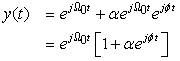
A complex signal y(t) is defined as
Solution
Since  , then using Euler's identity:

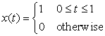
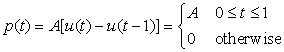
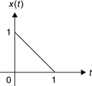
Consider the pulse signal
Solution
The analog signal p(t) is of finite support and real-valued. We have that
Example 1.1, Example 1.2 and Example 1.3 not only illustrate how different types of signal can be related to each other, but also how signals can be be defined in shorter or more precise forms. Although the representations for y(t) in Example 1.2 and in this example are equivalent, the one here is shorter and easier to visualize by the use of the pulse p(t).
1.3.1. Basic Signal Operations—Time Shifting and Reversal
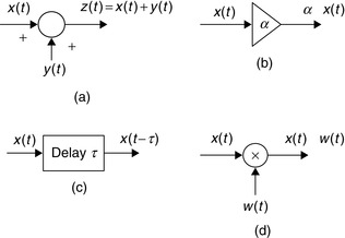
The following are basic signal operations used in the representation and processing of signals (for some of these operations we indicate the system that is used to realize the operation):
■ Signal addition—Two signals x(t) and y(t) are added to obtain their sum z(t). An adder is used.
■ Constant multiplication—A signal x(t) is multiplied by a constant α. A constant multiplier is used.
■ Time and frequency shifting—The signal x(t) is delayed τ seconds to get x(t − τ), and advanced by τ to get x(t + τ). A signal can be shifted in frequency or frequency modulated by multiplying it by a complex exponential or a sinusoid. A delay shifts right a time signal, while a modulator shifts the signal in frequency.
■ Time scaling—The time variable of a signal x(t) is scaled by a constant α to give x(αt). If α = −1, the signal is reversed in time (i.e., x(−t)), or reflected. Only the delay can be implemented in practice.
■ Time windowing—A signal x(t) is multiplied by a window signal w(t) so that x(t) is available in the support of w(t).
Given the simplicity of the first two operations we will only discuss the others. In this section we consider time shifting and reflection (a special case of the time scaling) and leave the rest for a later section.
In Figure 1.3 we show the diagrams used for the implementation of the addition of two signals, the multiplication of a signal by a constant, the delay of a signal, and the time windowing or modulation of a signal. These will be used in the block diagrams for systems in the next chapters.
 |
| Figure 1.3 |
It is important to understand that advancing or reflecting cannot be implemented in real time—that is as the signal is being processed. Delays can be implemented in real time. Advancing and reflection require that the signal be saved or recorded. Thus, an acoustic signal recorded on magnetic tape can be delayed or advanced with respect to an initial time, or played back, faster or slower, but it can only be delayed if we have the signal coming from a live microphone.
We will see later in this chapter that shifting in frequency results in the process of signal modulation, which is of great significance in communications. Scaling of the time variable results in a contracted and expanded version of the original signal and causes changes in the frequency content of the signal.
■ For a positive value τ, a signal x(t − τ) is the original signal x(t) shifted right or delayed τ seconds, as illustrated in Figure 1.4(b). That the original signal has been shifted to the right can be verified by finding that the x(0) value of the original signal appears in the delayed signal at t = τ (which results from making t − τ = 0).

■ Likewise, a signal x(t + τ) is the original signal x(t) shifted left or advanced by τ seconds as illustrated in Figure 1.4(c). The original signal is now shifted to the left—that is, the value x(0) of the original signal occurs now earlier (i.e., it has been advanced) at time t = −τ.
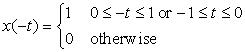
■ Reflection consists in negating the time variable. Thus, the reflection of x(t) is x(−t). This operation can be visualized as flipping the signal about the origin. See Figure 1.4(d).
Given an analog signal x(t) and τ > 0 we have that with respect to x(t):
Remarks
Whenever we combine the delaying or advancing with reflection, delaying and advancing are swapped. Thus, x(−t + 1) is x(t) reflected and delayed, or shifted to the right, by 1. Likewise, x(−t − 1) is x(t) reflected and advanced, or shifted to the left by 1. Again, the value x(0) of the original signal is found in x(−t + 1) at t = 1, and in x(−t − 1) at t = −1.
Consider an analog pulse
Solution
The delayed signal x(t − 2) can be found mathematically by replacing the variable t by t − 2 so that


Finally, the signal x(−t) is given by
When the shifting and reflecting operations are considered together the best approach to visualize the operation is to make a table computing several values of the new signal and comparing these with those from the original signal. Consider the pulse in Example 1.4 and plot the signal x(−t + 2).
Solution
Although one can see that this signal is reflected, it is not clear whether it is advanced or delayed by 2. By computing a few values:
| t | x(−t + 2) |
|---|---|
| 2 | x(0) = 1 |
| 1.5 | x(0.5) = 1 |
| 1 | x(1) = 1 |
| 0 | x(2) = 0 |
| −1 | x(3) = 0 |
Remarks
When computing the convolution integral later on, we will consider the signal x(t − τ) as a function of τ for different values of t. As indicated fromExample 1.5, this signal is a reflected version of x(τ) being shifted to the right t seconds. To see this, consider t = 0 then x(t − τ)|t=0 = x(−τ), the reflected version, and x(0) occurs at τ = 0. When t = 1, then x(t − τ)|t=1 = x(1 − τ) and x(0) occurs at τ = 1, so that x(1 − τ) is x(−τ) shifted to the right by 1, and so on.
1.3.2. Even and Odd Signals
Symmetry with respect to the origin differentiates signals and will be useful in their Fourier analysis. We have that an analog signal x(t) is called
■ Even whenever x(t) coincides with its reflection x(−t). Such a signal is symmetric with respect to the time origin.
■ Odd whenever x(t) coincides with −x(−t)—that is, the negative of its reflection. Such a signal is asymmetric with respect to the time origin.
Even and odd signals are defined as follows:
(1.4)
(1.5)
(1.6)
(1.7)
(1.8)
Using the definitions of even and odd signals, any signal y(t) can be decomposed into the sum of an even and an odd function. Indeed, the following is an identity:
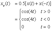
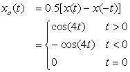
Consider the analog signal
Solution
1. x(t) is even if x(t = x(−t) or
2. for x(t) to be odd, we need that x(t) = −x(−t) or
When θ = π/4, x(t) = cos(2π t + π/4) is neither even nor odd according to the above.
Consider the signal

Solution
The signal x(t) is neither even nor odd given that its values for t ≤ 0 are zero. For its even–odd decomposition, the even component is given by

1.3.3. Periodic and Aperiodic Signals
A useful characterization of signals is whether they are periodic or aperiodic (nonperiodic).
An analog signal x(t) is periodic if
■ it is defined for all possible values of t, −∞ < t < ∞, and
■ there is a positive real value T0, the period of x(t), such that
(1.9)
The period of x(t) is the smallest possible value of T0 > 0 that makes the periodicity possible. Thus, although NT0 for an integer N > 1 is also a period of x(t) it should not be considered the period.
Remarks
■ The infinite support and the unique characteristic of the period make periodic signals nonexistent in practical applications. Despite this, periodic signals are of great significance in the Fourier representation of signals and in their processing, as we will see later. The representation of aperiodic signals is obtained from that of periodic signals, and the response of systems to periodic sinusoids is fundamental in the theory of linear systems.
■ Although seemingly redundant, the first part of the definition of a periodic signal indicates that it is not possible to have a nonzero periodic signal with a finite support (i.e., the analog signal is zero outside an interval t ∈ [t1, t2]). This first part of the definition is needed for the second part to make sense.
■ It is exasperating to find the period of a constant signal x(t) = A; visually x(t) is periodic but its period is not clear. Any positive value could be considered the period, but none will be taken. The reason is that x(t) = A = A cos(0t) or of zero frequency, and as such its period is not determined since we would have to divide by zero—not permitted. Thus, a constant signal is a periodic signal of nondefinable period!
Consider the analog sinusoid
Solution
The analog frequency is Ω0 = 2π/T0 so T0 = 2π/Ω0 is the period. Whenever T0 > 0 (or Ω0 > 0) these sinusoidals are periodic. For instance, consider
Consider a periodic signal x(t) of period T0. Determine whether the following signals are periodic, and if so, find their corresponding periods:
(a) y(t) = A + x(t).
(b) z(t) = x(t) + v(t) where v(t) is periodic of period T1 = NT0, where N is a positive integer.
(c) w(t) = x(t) + u(t) where u(t) is periodic of period T1, not necessarily a multiple of T0. Determine under what conditions w(t) could be periodic.
Solution
(a) Adding a constant to a periodic signal does not change the periodicity, so y(t) is periodic of period T0—that is, for an integer k, y(t + kT0) = A + x(t + kT0) = A + x(t) since x(t) is periodic of period T0.
(b) The period T1 = NT0 of v(t) is also a period of x(t), and so z(t) is periodic of period T1 since for any integer k,
Let x(t) = ej2t and y(t) = ejπ t, and consider their sum z(t) = x(t) + y(t), and their product w(t) = x(t)y(t). Determine if z(t) and w(t) are periodic, and if so, find their periods. Is p(t) = (1 + x(t))(1 + y(t)) periodic?
Solution
According to Euler's identity,
For z(t) to be periodic requires that T1/T0 be a rational number, which is not the case as T1/T0 = 2/π. So z(t) is not periodic.
The product is w(t) = x(t)y(t) = ej(2+π)t = cos(Ω2t) + j sin(Ω2t) where Ω2 = 2 + π = 2π/T2 so that T2 = 2π/(2 + π), so w(t) is periodic of period T2.
The terms 1 + x(t) and 1 + y(t) are periodic of period T0 = π and T1 = 2, and from the case of the product above, one would hope this product be periodic. But since p(t) = 1 + x(t) + y(t) + x(t)y(t) and x(t) + y(t) is not periodic, then p(t) is not periodic.
■ Analog sinusoids of frequency Ω0 > 0 are periodic of period T0 = 2π/Ω0. If Ω0 = 0, the period is not well defined.
■ The sum of two periodic signals x(t) and y(t), of periods T1 and T2, is periodic if the ratio of the periods T1/T2 is a rational number N/M, with N and M being nondivisible. The period of the sum is MT1 = NT2.
■ The product of two sinusoids is periodic. The product of two periodic signals is not necessarily periodic.
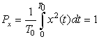
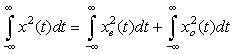
1.3.4. Finite-Energy and Finite Power Signals
Another possible classification of signals is based on their energy and power. The concepts of energy and power introduced in circuit theory can be extended to any signal. Recall that for a resistor of unit resistance its instantaneous power is given by

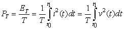
The energy and the power of an analog signal x(t) are defined for either finite or infinite-support signals as:
(1.10)
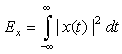
(1.11)
The signal x(t) is then said to be finite energy, or square integrable, whenever
(1.12)
(1.13)
Remarks
■ The above definitions of energy and power are valid for any signal of finite or infinite support, since a finite-support signal is zero outside its support.
■ In the formulas for energy and power we are considering the possibility that the signals might be complex and so we are squaring its magnitude: If the signal being considered is real, this simply is equivalent to squaring the signal.
■ According to the above definitions, a finite-energy signal has zero power. Indeed, if the energy of the signal is some constant Ex < ∞, then

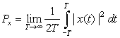
Find the energy and the power of the following:
(a) The periodic signal x(t) = cos(π t/2 + π/4).
(b) The complex signal y(t) = (1 + j)ejπ t/2, for 0 ≤ t ≤ 10 and zero otherwise.
(c) The pulse z(t) = 1, for 0 ≤ t ≤ 10 and zero otherwise.
Determine whether these signals are finite energy, finite power, or both.
Solution
The energy in these signals is computed as follows:
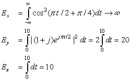
Using the trigonometric identity

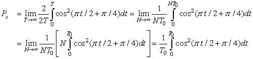
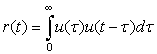
Consider an aperiodic signal x(t) = e−at, a > 0, for t ≥ 0 and zero otherwise. Find the energy and the power of this signal and determine whether the signal is finite energy, finite power, or both.
Solution
The energy of x(t) is given by
Consider the following analog signal, which we call a causal sinusoid because it is zero for t < 0:


As we will see later in the Fourier series representation, any periodic signal is representable as a possibly infinite sum of sinusoids of frequencies multiples of the fundamental frequency of the periodic signal being represented. These frequencies are said to be harmonically related, and for this case the power of the signal is shown to be the sum of the power of each of the sinusoidal components—that is, there is superposition of the power. This superposition is still possible when a sum of sinusoids creates a nonperiodic signal. This is illustrated in Example 1.14.
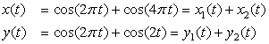
Consider the signals x(t) = cos(2π t) + cos(4π t) and y(t) = cos(2π t) + cos(2t), −∞ < t < ∞. Determine if these signals are periodic, and if so, find their periods. Compute the power of these signals.
Solution
The sinusoids cos(2πt) and cos(4πt) periods T1 = 1 and T2 = 1/2, so x(t) is periodic since T1/T2 = 2 with period T1 = 2T2 = 1. The two frequencies are harmonically related. The sinusoid cos(2t) has as period T3 = π. Therefore, the ratio of the periods of the sinusoidal components of y(t) is T1/T3 = 1/π, which is not rational, and so y(t) is not periodic and the frequencies 2π and 2 are not harmonically related.
Using the trigonometric identities
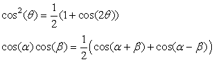


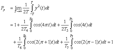
The power of a sum of sinusoids,
(1.15)
(1.16)
1.4. Representation Using Basic Signals
A fundamental idea in signal processing is to attempt to represent signals in terms of basic signals, which we know how to process. In this section we consider some of these basic signals (complex exponentials, sinusoids, impulse, unit-step, and ramp) that will be used to represent signals and for which we will obtain their responses in a simple way in the next chapter.
1.4.1. Complex Exponentials
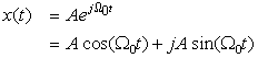
A complex exponential is a signal of the form
(1.17)
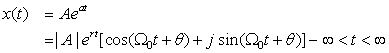
Using Euler's identity, ejϕ = cos(ϕ) + j sin(ϕ), and from the definitions of A and a as complex numbers, we have that

Remarks
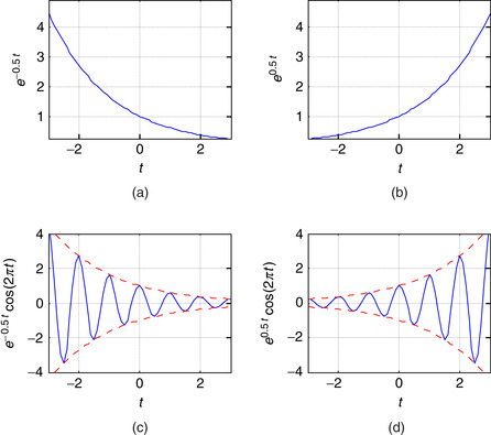
■ Suppose that A and a are real, then
■ If both A and a are complex, x(t) is a complex signal and we need to consider separately its real and imaginary parts. For instance, the real part function is

The envelope of g(t) can be found by considering that
■ According to the above, several signals can be obtained from the complex exponential.
 |
| Figure 1.5 |
Sinusoids
Sinusoids are of the general form
(1.18)
The cosine and the sine signals, as indicated above, are out of phase by π/2 radians. The frequency can also be expressed in hertz or 1/sec units, and in that case Ω0 = 2π f0, and the period is found by the relation f0 = 1/T0 (it is important to point out the inverse relation between time and frequency shown here, which will be important in the representation of signals later on).
Recall from Chapter 0, that the Euler's identity provides the relation of the sinusoids with the complex exponential
(1.19)
(1.20)
(1.21)
Remarks
A sinusoid is characterized by its amplitude, frequency, and phase. When we allow these three parameters to be functions of time, or
■ Amplitude modulation (AM)—The amplitude A(t) changes according to the message, while the frequency and the phase are constant,
■ Frequency modulation (FM)—The frequency Ω(t) changes according to the message, while the amplitude and phase are constant,
■ Phase modulation (PM)—The phase θ(t) varies according to the message and the other parameters are kept constant.
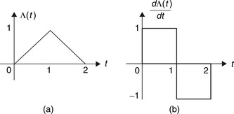
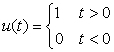
1.4.2. Unit-Step, Unit-Impulse, and Ram Signals
Unit-Step and Unit-Impulse Signals
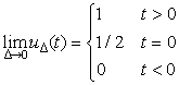
Consider a rectangular pulse of duration Δ and unit area
(1.22)

(1.23)

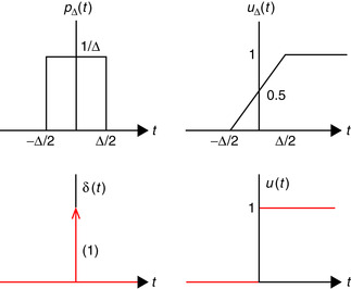
Suppose that Δ → 0, then
■ The pulse pΔ(t) still has a unit area but is an extremely narrow pulse. We will call the limit the unit-impulse signal,
(1.24)
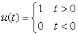
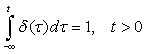
You can think of the u(t) as the switching of a dc signal generator from off to on, while δ(t) is a very strong pulse of very short duration.
The impulse signal δ(t) is:
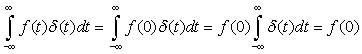
■ Zero everywhere except at the origin where its value is not well defined (i.e., δ(t) = 0, t ≠ 0, and undefined at t = 0).
■ its area is unity, i.e.,
(1.26)
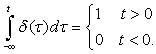
The unit-step signal is

(1.27)

(1.28)
According to calculus we have

Remarks
■ Since u(t) is not a continuous function, it jumps from 0 to 1 instantaneously around t = 0, from the calculus point of view it should not have a derivative. That δ(t) is its derivative must be taken with suspicion, which makes the δ(t) signal also suspicious. Such signals can, however, be formally defined using the theory of distributions.
■ The impulse δ(t) is impossible to generate physically, but characterizes very brief pulses of any shape. It can be derived using pulses or functions different from the rectangular pulse (seeEq. 1.22). InProblem 1.7at the end of the chapter it is indicated how it can be derived from either a triangular pulse or a sinc function of unit area.
■ Signals with jump discontinuities can be represented as the sum of a continuous signal and unit-step signals at the discontinuities. This is useful in computing the derivative of these signals.
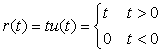
Ramp Signal
The ramp signal is defined as
(1.29)
(1.30)
(1.31)
The ramp is a continuous function and its derivative is given by
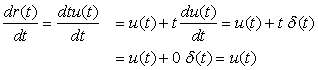
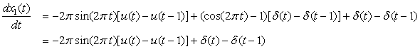
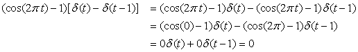
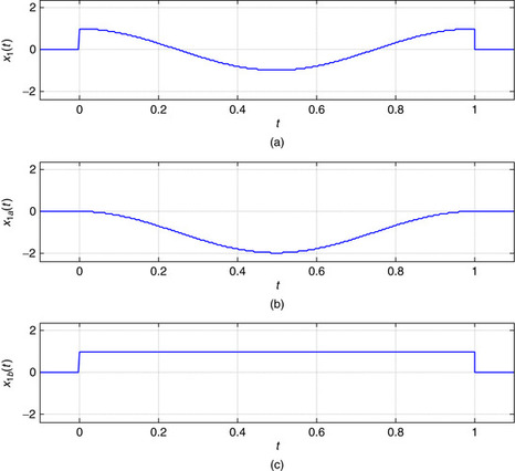
Consider the discontinuous signals
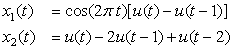
Solution
The signal x1(t) is a period of a cosine of period T0 = 1, 0 ≤ t ≤ 1, with a discontinuity of 1 at t = 0 and t = 1. Subtracting u(t) − u(t − 1) from x1(t) we obtain a continuous signal, but to compensate we must add a unit pulse between t = 0 and t = 1, giving
 |
| Figure 1.7 |
The signal x2(t) has jump discontinuities at t = 0, t = 1, and t = 2, and we can think of it as completely discontinuous so that its continuous component is 0. The derivative is
Signal Generation with MATLAB
In the following examples we illustrate how to generate analog signals using MATLAB. This is done by either approximating continuous-time signals by discrete-time signals or by using the symbolic toolbox. The function plot uses an interpolation algorithm that makes the plots of discrete-time signals look like analog signals.
Write a script and the necessary functions to generate a signal,
Solution
We wrote functions ramp and ustep to generate ramp and unit-step signals for obtaining a numeric approximation of the signal y(t). The following script shows how these functions are used to generate y(t). The arguments of ramp determine the support of the signal, the slope, and the shift (for advance, a positive number, and for delay, a negative number). For ustep we need to provide the support and the shift.
%%%%%%%%%%%%%%%%%%%
% Example 1.16
%%%%%%%%%%%%%%%%%%%
clear all; clf
Ts = 0.01; t = -5:Ts:5; % support of signal
% ramp with support [-5, 5], slope of 3 and advanced
% (shifted left) with respect to the origin by 3
y1 = ramp(t,3,3);
y2 = ramp(t,-6,1);
y3 = ramp(t,3,0);
% unit-step function with support [-5,5], delayed by 3
y4 = -3* ustep(t,-3);
y = y1 + y2 + y3 + y4;
plot(t,y,’k’); axis([-5 5 -1 7]); grid
Our functions ramp and ustep are as follows.
function y = ramp(t,m,ad)
% ramp generation
% m: slope of ramp
% ad : advance (positive), delay (negative) factor
% USE: y = ramp(t,m,ad)
N = length(t);
y = zeros(1,N);
for i = 1:N,
if t(i)>= -ad,
y(i) = m*(t(i)+ad);
end
end
function y=ustep(t,ad)
% generation of unit step
% t: time
% ad : advance (positive), delay (negative)
% USE y = ustep(t,ad)
N = length(t);
y = zeros(1,N);
for i = 1:N,
if t(i) >= -ad,
y(i) = 1;
end
end
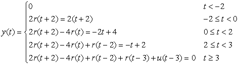
Analytically,
■ y(t) = 0 for t < −3 and for t > 3, so the chosen support −5 ≤ t ≤ 5 displays the signal in a region where the signal occurs.
■ For −3 ≤ t ≤ −1, y(t) is 3r(t + 3) = 3(t + 3), which is 0 at t = −3 and 6 at t = −1.
■ For −1 ≤ t ≤ 0, y(t) is 3r(t + 3) − 6r(t + 1) = 3(t + 3) − 6(t + 1) = −3t + 3, which is 6 at t = −1 and 3 at t = 0.
■ For 0 ≤ t ≤ 3, y(t) is 3r(t + 3) − 6r(t + 1) + 3r(t) = −3t + 3 + 3t = 3.
■ For t ≥ 3 the signal is 3r(t + 3) − 6r(t + 1) + 3r(t) − 3u(t − 3) = 3 − 3 = 0.
These coincide with the signal shown in Figure 1.8.

Consider the following script that uses the functions ramp and ustep to generate a signal y(t). Obtain analytically the formula for the signal y(t). Write a function to compute and plot the even and odd components of y(t).
clear all; clf
t = -5:0.01:5;
y1 = ramp(t,2,2.5);
y2 = ramp(t,-5,0);
y4 = ustep(t,-4);
y = y1 + y2 + y3 + y4;
plot(t,y,’k’); axis([-5 5 -3 5]); grid
The signal y(t) = 0 for t < −5 and t > 5.
Solution
The signal y(t) displayed on Figure 1.9(a) is given analytically by
 |
| Figure 1.9 |
%%%%%%%%%%%%%%%%%%%
% Example 1.17
%%%%%%%%%%%%%%%%%%%
[ye, yo] = evenodd(t,y);
subplot(211)
plot(t,ye,’r’)
grid
axis([min(t) max(t) -2 5])
subplot(212)
plot(t,yo,’r’)
axis([min(t) max(t) -1 5])
function [ye,yo] = evenodd(t,y)
% even/odd decomposition
% t: time
% y: analog signal
% ye, yo: even and odd components
% USE [ye,yo] = evenodd(t,y)
%
yr = fliplr(t,y);
ye = 0.5*(y + yr);
yo=0.5*(y - yr);
The MATLAB function fliplr reverses the values of the vector y giving the reflected signal.
Use symbolic MATLAB to generate the following analog signals.
(a) For the damped sinusoid signal
(b) For a rough approximation of a periodic pulse generated by adding three cosines of frequencies multiples of Ω0 = π/10—that is
Solution
The following script generates the damped sinusoid signal, and its envelope y(t) = ±e−t.
%%%%%%%%%%%%%%%%%%%
% Example 1.18 --- damped sinusoid
%%%%%%%%%%%%%%%%%%%
t = sym(’t’);
x = exp(-t)*cos(2*pi*t);
y = exp(-t);
ezplot(x,[-2,4])
grid
ezplot(y,[-2,4])
hold on
ezplot(-y,[-2,4])
axis([-2 4 -8 8])
hold off
The approximate pulse signal is generated by the following script.
clear; clf
t = sym(’t’);
% sum of constant and cosines
x = 1 + 1.5*cos(2*pi*t/10)-.6*cos(4*pi*t/10);
ezplot(x,[-10,10]); grid
The plots of the damped sinusoid and the approximate pulse are given in Figure 1.10.

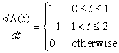
Consider the generation of a triangular signal,

Solution
The triangular pulse can be represented as
(1.32)

Using the mathematical definition of the triangular function, its derivative is given by
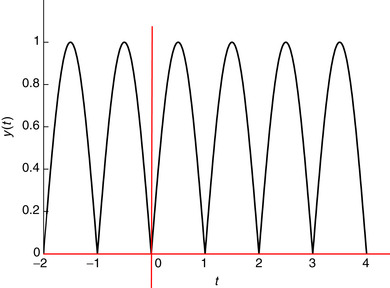
Consider a full-wave rectified signal,

Solution
The period between 0 and 0.5 can be expressed as
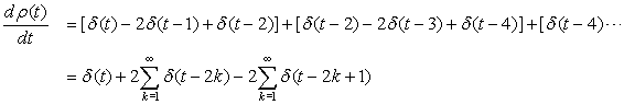
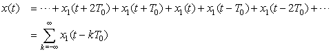
Generate a causal train of pulses that repeats every two units of time using as first period
Solution
Considering that s(t) is the first period of the train of pulses of period two, then


1.4.3. Special Signals—the Sampling Signal and the Sinc
Two signals of great significance in the sampling of continuous-time signals and their reconstruction are the sampling signal and the sinc. Sampling a continuous-time signal consists in taking samples of the signal at uniform times. One can think of this process as the multiplication of a continuous-time signal x(t) by a train of very narrow pulses of the sampling period Ts. For simplicity, considering that the width of the pulses is much smaller than Ts, the train of pulses can be approximated by a train of impulses that is periodic of period Ts—that is, the sampling signal is
is
(1.33)
(1.34)

A fundamental result in sampling theory is the recovery of the original signal, under certain constrains, by means of an interpolation using sinc signals. Moreover, we will see that the sinc is connected with ideal low-pass filters. The sinc function is defined as
(1.35)
■ The time support of this signal is infinite.
■ It is an even function of t, as
(1.36)
■ At t = 0 the numerator and the denominator of the sinc are zero; thus the limit as t → 0 is found using L'Hˆopital's rule—that is,
(1.37)
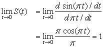
■ S(t) is bounded—that is, since −1 ≤ sin(π t) ≤ 1, then for t ≥ 0,
(1.38)
■ The zero-crossing time of S(t) are found by letting the numerator equal zero—that is, when sin(π t) = 0, the zero-crossing times are such that π t = kπ, or t = k for a nonzero integer k or k = ±1, ±2, ….
■ A property that is not obvious and that requires the frequency representation of S(t) is that the integral
(1.39)
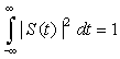
The sinc signal will appear in several places in the rest of the book.
1.4.4. Basic Signal Operations—Time Scaling, Frequency Shifting, and Windowing
Given a signal x(t), and real values α ≠ 0 or 1, and ϕ > 0:
■ x(αt) is said to be contracted if |α| > 1, and if α < 0 it is also reflected.
■ x(αt) is said to be expanded if |α| < 1, and if α < 0 it is also reflected.
■ x(t)ejϕt is said to be shifted in frequency by ϕ radians.
■ For a window signal w(t), x(t)w(t) displays x(t) within the support of w(t).
To illustrate the time scaling, consider a signal x(t) with a finite support t0 ≤ t ≤ t1. Assume that α > 1, then x(αt) is defined in t0 ≤ αt ≤ t1 or t0/α ≤ t ≤ t1/α, a smaller support than the original one. For instance, for α = 2, t0 = 2, and t1 = 4, then the support of x(2t) is 1 ≤ t ≤ 2, while the support of x(t) is 2 ≤ t ≤ 4. If α = −2, then x(−2t) is not only contracted but also reflected. Similarly, x(0.5t) would have a support of 2t0 ≤ t ≤ 2t1, which is larger than the original support.
Multiplication by an exponential shifts the frequency of the original signal. To illustrate this consider the case of an exponential x(t) = ejΩ0t of frequency Ω0. If we multiply x(t) by an exponential ejϕt, then
Notice that time scaling also changes the frequency content of the signal. For instance, a signal  is periodic of period T0 = 2π/Ω0, while
  has a period T0/α or a frequency αΩ0, which is larger than the original frequency of Ω0 when α > 1 and smaller than Ω0 when 0 < α < 1.
Remarks
We can thus summarize the above as follows:
■ If x(t) is periodic of period T0then the time-scaled signal x(αt), α ≠ 0, is also periodic of period T0/|α|.
■ The support in time of a periodic or nonperiodic signal is inversely proportional to the support in frequency for that signal.
■ The frequencies present in a signal can be changed by modulation—that is, multiplying the signal by a complex exponential or, equivalently, by sines and cosines. The frequency change is also possible by expansion and compression of the signal.
■ Reflection is a special case of time scaling with α = −1.
Let x1(t), for 0 ≤ t ≤ T0, be one period of a periodic signal x(t) of period T0. Represent x(t) in terms of advanced and delayed versions of x1(t). What would be x(2t)?
Solution
The periodic signal x(t) can be written as
An acoustic signal x(t) has a duration of 3.3 minutes and a radio station would like to use the signal for a three-minute segment. Indicate how to make it possible.
Solution
We need to contract the signal by a factor of α = 3.3/3 = 1.1, so that x(1.1t) can be used in the three-minute piece. If the signal is recorded on tape, the tape player can be run 1.1 times faster than the recording speed. This would change the voice or music on the tape, as the frequencies x(1.1t) are increased with respect to the original frequencies in x(t).
One way of transmitting a message over the airwaves is to multiply it by a sinusoid of frequency higher than those in the message, thus changing the frequency content of the signal. The resulting signal is called an amplitude-modulated (AM) signal: The message changes the amplitude of the sinusoid. To recover the message from the transmitted signal, one can make the envelope of the modulated signal be related to the message. Use again the ramp and ustep functions to generate a signal y(t) = 2r(t + 2) − 4r(t) + r(t − 2) + r(t − 3) + u(t − 3) to modulate a so-called carrier signal x(t) = sin(5π t) to give the AM signal z(t). Obtain a script to generate and plot the AM signal. Indicate whether the envelope of the AM signal is connected with the message signal y(t).
Solution
The signal y(t) analytically equals
The following script is used to generate the message signal y(t), the AM signal z(t), and the corresponding plots. The MATLAB function sound is used to produce the sound corresponding to 100z(t). In Figure 1.14 we show z(t) and emphasize the envelope (dashed line) that corresponds to ±y(t).

%%%%%%%%%%%%%%%
% Example 1.24 --- AM signal
%%%%%%%%%%%%%%%
t = -5:0.01:5;
x = sin(5*pi*t);
y1 = ramp(t,2,2);
y2 = ramp(t,-4,0);
y3 = ramp(t,1,-2);
y4 = ramp(t,1,-3);
y5 = ustep(t,-3);
y = y1 + y2 + y3 + y4 + y5;
z = y.*x;
sound(100*z,1000)
plot(t,z,’k’); hold on
plot(t,y,’r’,t,-y,’r’); axis([-5 5 -5 5]); grid
hold off
xlabel(’t’); ylabel(’z(t)’)
1.4.5. Generic Representation of Signals
Consider the following integral:

(1.40)
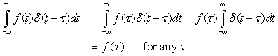

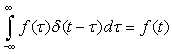
By the sifting property of the impulse function δ(t), any signal x(t) can be represented by the following generic representation:
(1.41)
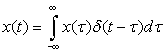
Figure 1.16 shows a generic representation. Equation (1.41) basically indicates that any signal can be viewed as a stacking of pulses x(kΔ)pΔ(t − kΔ), which in the limit as Δ → 0 become impulses x(τ)δ(t − τ).
 |
| Figure 1.16 |
Equation (1.41) provides a generic representation of a signal in terms of basic signals, in this case impulse signals. As we will see in the next chapter, once we determine the response of a system to an impulse we will use the generic representation to find the response of the system to any signal.
1.5. What Have We Accomplished? Where Do We Go from Here?
We have taken another step in our long journey. In this chapter we discussed the main classification of signals and have started the study of deterministic, continuous-time signals. We have also discussed important characteristics of signals such as periodicity, energy, power, evenness, and oddness, and learned basic signal operations that will be useful as we will see in the next chapters. Interestingly, we began to see how some of these operations lead to practical applications, such as amplitude, frequency, and phase modulations, which are basic in the theory of communications. Very importantly, we have also begun to represent signals in terms of basic signals, which in later chapters will allow us to simplify the analysis and will give us flexibility in the synthesis of systems. These basic signals are used as test signals in control systems. Table 1.1 displays basic signals.


Our next step is to connect signals with systems. We are particularly interested in developing a theory that can be used to approximate, to some degree, the behavior of most systems of interest in engineering. After that we consider the analysis of signals and systems time and frequency domains.
Signal Energy and RC Circuit—MATLAB
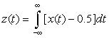
 and determine if it is finite.
 is finite, could you say that x(t) has finite energy? Explain why or why not. Hint: Plot |x(t)| and |x(t)|2 as functions of time.
 is less than half the energy of x(t)? Explain. To verify your result, use symbolic MATLAB to plot y(t) and to compute its energy.
The signal x(t) = e−|t| is defined for all values of t.
(a) Plot the signal x(t) and determine if this signal is finite energy. That is, compute the integral
(b) If you determine that x(t) is absolutely integrable, or that the integral
(c) From your results above, is it true the energy of the signal
(d) To discharge a capacitor of 1 mF charged with a voltage of 1 volt we connect it, at time t = 0, with a resistor of R Ω. When we measure the voltage in the resistor we find it to be vR(t) = e−tu(t). Determine the resistance R. If the capacitor has a capacitance of 1μF, what would be R? In general, how are R and C related?
Power in RL Circuits

 where Vs and I are the phasors corresponding to the source and the current in the circuit, and I∗ is the complex conjugate of I. Consider the values of the resistor and the inductor given above, and compute the complex power and relate it to the average power computed in each case.
Consider a circuit consisting of a sinusoidal source vs(t) = cos(t)u(t) volts connected in series to a resistor R and an inductor L and assume they have been connected for a very long time.
(a) Let R = 0 and L = 1 H. Compute the instantaneous and the average powers delivered to the inductor.
(b) Let R = 1 Ω and L = 1 H. Compute the instantaneous and the average powers delivered to the resistor and the inductor.
(c) Let R = 1 Ω and L = 0 H. Compute the instantaneous and the average powers delivered to the resistor. Hint: In the above parts of the problem use phasors or the trigonometric formula
(d) The average power used by the resistor is what you pay to the electric company, but there is also a reactive power for which you do not. The complex power supplied to the circuit is defined as
Power in Periodic and Nonperiodic Sum of Sinusoids
Consider the periodic signal x(t) = cos(2Ω0t) + 2cos(Ω0t), −∞ < t < ∞, and Ω0 = π. The frequencies of the two sinusoids are said to be harmonically related (one is a multiple of the other).
(b) Compute the power Px of x(t).
(c) Verify that the power Px is the sum of the power P1 of x1(t) = cos(2π t) and the power P2 of x2(t) = 2cos((π t).
(d) In the above case you are able to show that there is superposition of the powers because the frequencies are harmonically related. Suppose that y(t) = cos(t) + cos(π t) where the frequencies are not harmonically related. Find out whether y(t) is periodic or not. Indicate how you would find the power Py of y(t). Would Py = P1 + P2 where P1 is the power of cos(t) and P2 is the power of cos(π t)? Explain what is the difference with respect to the case of harmonic frequencies.
Periodicity of Sum of Sinusoids—MATLAB
Consider the periodic signals x1(t) = 4cos(π t) and x2(t) = −sin(3π t + π/2).
(a) Find the periods of x1(t) and x2(t).
(b) Is the sum x(t) = x1(t) + x2(t) periodic? If so, what is its period?
(c) In general, two periodic signals x1(t) and x2(t) having periods T1 and T2 such that their ratio T1/T2 = M/K is a rational number (i.e., M and K are positive integers), then the sum x(t) = x1(t) + x2(t) is periodic. Suppose the rationality condition is satisfied and M = 3 and K = 12. Determine the period of x(t).
(d) Determine whether x(t) = x1(t) + x2(t) is periodic when
■ x1(t) = 4cos(2π t) and x2(t) = −sin(3π t + π/2)
■ x1(t) = 4cos(2t) and x2(t) = −sin(3π t + π/2)
Use symbolic MATLAB to plot x(t) in the above two cases and confirm your analytic results about the periodicity or lack of periodicity of x(t).
Time Shifting
 and zero elsewhere.
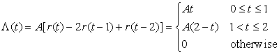
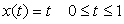
Consider a finite-support signal
(a) Carefully plot x(t + 1).
(b) Carefully plot x(−t + 1).
(c) Add the above two signals to get a new signal y(t). To verify your results, represent each of the above signals analytically and show that the resulting signal is correct.
(d) How does y(t) compare to the signal Λ(t) = (1 − |t|)(u(t + 1) − u(t − 1)? Plot them. Compute the integrals of y(t) and Λ(t) for all values of t and compare them. Explain.
Even and Odd Hyperbolic Functions—MATLAB
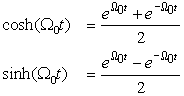
According to Euler's identity the sine and the cosine are defined in terms of complex exponentials. You would then ask what if instead of complex exponentials you were to use real exponentials. Well, using Euler's identity we obtain the hyperbolic functions defined in −∞ < t < ∞:
(a) Let Ω0 = 1 rad/sec. Use the definition of the real exponentials to plot cosh(t) and sinh(t).
(b) Is cosh(t) even or odd?
(d) Obtain an expression for x(t) = e−tu(t) in terms of the hyperbolic functions. Use symbolic MATLAB to plot x(t) = e−tu(t) and to plot your expression in terms of the hyperbolic functions. Compare them.
Impulse Signal Generation—MATLAB
 Carefully plot it, compute its area, and find its limit as Δ → 0. What do you obtain in the limit? Explain.
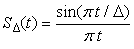 Use the properties of the sinc signal S(t) = sin(π t)/(π t) to express SΔ(t) in terms of S(t). Then find its area, and the limit as Δ → 0. Use symbolic MATLAB to show that for decreasing values of Δ the SΔ(t) becomes like the impulse signal.
When defining the impulse or δ(t) signal, the shape of the signal used to do so is not important. Whether we use the rectangular pulse we considered in this chapter or another pulse, or even a signal that is not a pulse, in the limit we obtain the same impulse signal. Consider the following cases:
(a) The triangular pulse,
(b) Consider the signal
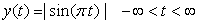
Impulse and Unit-Step Signals
 and a causal sinusoid defined as
 where the unit-step function indicates that the function has a discontinuity at zero, since for t = 0+ the function is close to 1, and for t = 0− the function is zero.
By introducing the impulse δ(t) and the unit-step u(t) signals, we expand the conventional calculus. One of the advantages of having the δ(t) function is that we are now able to find the derivative of discontinuous signals. Let us illustrate this advantage. Consider a periodic sinusoid defined for all times,
(a) Find the derivative y(t) = dx(t)/dt and plot it.
(b) Find the derivative z(t) = dx1(t)/dt (treat x1(t) as the product of two functions cos(Ω0t) and u(t)) and plot it. Express z(t) in terms of y(t).
(c) Verify that the integral of z(t) gives you back x1(t).
Series RC Circuit Response to a Unit-Step Signal
A unit-step function u(t) can be considered a causal constant source (e.g., a battery in a circuit if the units of u(t) is volts).
(a) From basic principles consider the response of an RC circuit to u(t)—that is, a battery connected in series with the resistor and the capacitor. Remember that the voltage across the capacitor results from an accumulation of charge, and that the presence of the resistor simply means that the charge is slowly accumulated. Therefore, plot what would be the voltage across the capacitor for t > 0 (assume the capacitor has no initial voltage at t = 0).
(b) What would be the voltage across the capacitor in the steady state? Explain.
(c) Finally, suppose that the capacitor is disconnected from the circuit at some time t0 ≫ 0. Ideally, what would be the voltage across the capacitor from then on?
(d) If you disconnect the capacitor, again at t0 ≫ 0, but somehow it is left connected to the resistor, so they are in parallel, what would happen to the voltage across the capacitor? Plot approximately the voltage across the capacitor for all times and explain the reason for your plot.
Ramp in Terms of Unit-Step Signals


 to show that
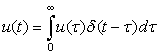
(a) Show that the above expression for r(t) is equivalent to
(b) Compute the derivative of
Sampling Signal and Impulse Signal—MATLAB
 which we will use in the sampling of analog signals later on.
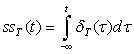 and carefully plot it for all t. What does the resulting signal ss(t) look like? In reference 17, Craig calls it the “stairway to the stars.” Explain.
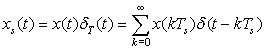 Let x(t) = cos(2π t)u(t) and Ts = 0.1. Find the integral
 and use MATLAB to plot it for 0 ≤ t ≤ 10. In a simple way this problem illustrates the operation of a discrete-to-analog converter, which converts a discrete-time into a continuous-time signal (its cousin is the digital-to-analog converter or DAC).
Consider the sampling signal
(a) Plot δT(t). Find
(b) Use MATLAB function stairs to plot ssT(t) for T = 0.1. Determine what signal would be the limit as T → 0.
(c) A sampled signal is
Reflection and Time Shifting
Do the reflection and the time-shifting operations commute? That is, do the two block diagrams in Figure 1.17 provide identical signals (i.e., is y(t) equal to z(t))? To provide an answer to this consider the signal x(t) shown in Figure 1.17. Reflect x(t) to get v(t) = x(−t) and then shift it to get y(t) = v(t − 2). Then consider delaying x(t) to get w(t) = x(t − 2), and reflecting it to get z(t) = w(−t). Perform each of these operations on x(t) to get y(t) and z(t); plot them and compare these plots. What is your conclusion? Explain
 |
| Figure 1.17 |
Contraction and Expansion of Signals
Let x(t) be the analog signal considered in Problem 1.12 (see Figure 1.17). In this problem we would like to consider expanded and compressed versions of that signal.
(a) Plot x(2t) and determine if it is a compressed or expanded version of x(t).
(b) Plot x(t/2) and determine if it is a compressed or expanded version of x(t).
(c) Suppose x(t) is an acoustic signal—let's say it is a music signal recorded in a magnetic tape. What would be a possible application of the expanding and compression operations? Explain.
Even and Odd Decomposition and Power
Consider the analog signal x(t) in Figure 1.18.
 |
| Figure 1.18 |
(a) Plot the even–odd decomposition of x(t)(i.e., find and plot the even xe(t) and the odd xo(t) components of x(t)).
(b) Show that the energy of the signal x(t) can be expressed as the sum of the energies of its even and odd components—that is, that
(c) Verify that the energy of x(t) is equal to the sum of the energies of xe(t) and xo(t).
Generation of Periodic Signals
A periodic signal can be generated by repeating a period.
(a) Find the function g(t), defined in 0 ≤ t ≤ 2 only, in terms of basic signals and such, that when repeated using a period of 2, generates the periodic signal x(t), as shown in Figure 1.19.
 |
| Figure 1.19 |
(b) Obtain an expression for x(t) in terms of g(t) and shifted versions of it.
(c) Suppose we shift and multiply by a constant the periodic signal x(t) to get new signals y(t) = 2x(t − 2), z(t) = x(t + 2), and v(t) = 3x(t). Are these signals periodic?
(d) Let then w(t) = dx(t)/dt, and plot it. Is w(t) periodic? If so, determine its period.
Contraction and Expansion and Periodicity—MATLAB
Consider the periodic signal x(t) = cos(π t) of period T0 = 2 sec.
(a) Is the expanded signal x(t/2) periodic? If so, indicate its period.
(b) Is the compressed signal x(2t) periodic? If so, indicate its period.
(c) Use MATLAB to plot the above two signals and verify your analytic results.
Derivatives and Integrals of Periodic Signals
Consider the triangular train of pulses x(t) in Figure 1.20.
 |
| Figure 1.20 |
Complex Exponentials
For a complex exponential signal x(t) = 2ej2π t:
(a) Determine its analog frequency Ω0 in rad/sec and its analog frequency f in hertz. Then find the signal's period.
(b) Suppose y(t) = ejπ t. Would the sum of these signals z(t) = x(t) + y(t) also be periodic? If so, what is the period of z(t)?
(c) Suppose we then generate a signal v(t) = x(t)y(t), with the x(t) and y(t) signals given before. Is v(t) periodic? If so, what is its period?
Full-Wave Rectified Signal—MATLAB
 part of which is shown in Figure 1.21.
Consider the full-wave rectified signal
 |
| Figure 1.21 |
(a) As a periodic signal, y(t) does not have finite energy, but it has a finite power Py. Find it.
(b) It is always useful to get a quick estimate of the power of a periodic signal by finding a bound for the signal squared. Find a bound for |y(t)|2 and show that Py < 1.
(c) Use symbolic MATLAB to check if the full-wave rectified signal has finite power and if that value coincides with the Py you found above. Plot the signal and provide the script for the computation of the power. How does it coincide with the analytical result?
Multipath Effects, First Part—MATLAB
 and let τ = 0.5 seconds. Determine the number of samples corresponding to a delay of τ seconds by using the sampling rate Fs(samples per second) given when the file “handel.mat” is loaded.
In wireless communications, the effects of multipath significantly affect the quality of the received signal. Due to the presence of buildings, cars, etc. between the transmitter and the receiver, the sent signal does not typically go from the transmitter to the receiver in a straight path (called line of sight). Several copies of the signal, shifted in time and frequency as well as attenuated, are received—that is, the transmission is done over multiple paths each attenuating and shifting the sent signal. The sum of these versions of the signal appears quite different from the original signal given that constructive as well as destructive effects may occur. In this problem we consider the time-shift of an actual signal to illustrate the effects of attenuation and time shift. In the next problem we consider the effects of time and frequency shifting and attenuation.
Assume that the MATLAB “handel.mat” signal is an analog signal x(t) that it is transmitted over three paths, so that the received signal is
To simplify matters, just work with a signal of duration 1 second—that is, generate a signal from “handel.mat” with the appropriate number of samples. Plot the segment of the original “handel.mat” signal x(t) and the signal y(t) to see the effect of multipath. Use the MATLAB function sound to listen to the original and the received signals.
Multipath Effects, Second Part—MATLAB
 where α is the attenuation and ϕ is the Doppler frequency shift, which is typically much smaller than the signal frequency. Let Ω0 = π, ϕ = π/100, and α = 0.7. This is analogous to the case where the received signal is the sum of the line-of-sight signal and an attenuated signal affected by Doppler.
 That is, the effects of time and frequency delays, put together with attenuation, for the times indicated in part (a). Use the function sound (let Fs = 2000 in this function) to listen to the different signals.
Consider now the Doppler effect in wireless communications. The difference in velocity between the transmitter and the receiver causes a shift in frequency in the signal, which is called the Doppler effect (e.g., this is just like the acoustic effect of a train whistle as a train goes by).
To illustrate the frequency-shift effect, consider a complex exponential  . Assume two paths: One that does not change the signal, while the other causes the frequency shift and attenuation, resulting in the signal
(a) Consider the term αejϕt, a phasor with frequency ϕ = π/100 to which we add 1. Use the MATLAB plotting function compass to plot the addition 1 + 0.7ejϕt for times from 0 to 256 sec, changing in increments of T = 0.5 sec.
(b) If we write  , give analytical expressions for A(t) and θ(t), and compute and plot them using MATLAB for the times indicated above.
(c) Compute the real part of the signal
Beating or Pulsation—MATLAB
 where the fi are frequencies from 159 to 161 separated by Δ Hz.
An interesting phenomenon in the generation of musical sounds is beating or pulsation. Suppose NP different players try to play a pure tone, a sinusoid of frequency 160 Hz, and that the signal recorded is the sum of these sinusoids. Assume the NP players while trying to play the pure tone end up playing tones separated by 0.02 Hz, so that the recorded signal is
(a) Generate the signal y(t) 0 ≤ t ≤ 200 sec in MATLAB. Let each musician play a unique frequency. Consider an increasing number of players, letting NP be first 51 players with Δ = 0.04 Hz, and then 101 players with Δ = 0.02 Hz. Plot y(t) for each of the different number of players.
(b) Explain how this is related with multipath and Doppler effects discussed in the previous problems.
Chirps—MATLAB
Pure tones or sinusoids are not very interesting to listen to. Modulation and other techniques are used to generate more interesting sounds. Chirps, which are sinusoids with time-varying frequency, are some of those more interesting sounds. For instance, the following is a chirp signal:
(a) Let A = 1, Ωc = 2, and s(t) = t2/4. Use MATLAB to plot this signal for 0 ≤ t ≤ 40 sec in steps of 0.05 sec. Use the sound function to listen to the signal.
(b) Let A = 1, Ωc = 2, and s(t) = −2 sin(t). Use MATLAB to plot this signal for 0 ≤ t ≤ 40 sec in steps of 0.05 sec. Use the sound function to listen to the signal.
(c) The frequency of these chirps is not clear. The instantaneous frequency IF(t) is the derivative with respect to t of the argument of the cosine. For instance, for a cosine cos(Ω0t), the IF(t) = dΩ0t/dt = Ω0, so that the instantaneous frequency coincides with the conventional frequency. Determine the instantaneous frequencies of the two chirps and plot them. Do they make sense as frequencies? Explain.
..................Content has been hidden....................
You can't read the all page of ebook, please click here login for view all page.