
Chapter 0. From the Ground Up!
In theory there is no difference between theory and practice. In practice there is.
Lawrence “Yogi” Berra, 1925 New York Yankees baseball player
This chapter provides an overview of the material in the book and highlights the mathematical background needed to understand the analysis of signals and systems. We consider a signal a function of time (or space if it is an image, or of time and space if it is a video signal), just like the voltages or currents encountered in circuits. A system is any device described by a mathematical model, just like the differential equations obtained for a circuit composed of resistors, capacitors, and inductors.
By means of practical applications, we illustrate in this chapter the importance of the theory of signals and systems and then proceed to connect some of the concepts of integro-differential Calculus with more concrete mathematics (from the computational point of view, i.e., using computers). A brief review of complex variables and their connection with the dynamics of systems follows. We end this chapter with a soft introduction to MATLAB, a widely used high-level computational tool for analysis and design.
Significantly, we have called this Chapter 0, because it is the ground floor for the rest of the material in the book. Not everything in this chapter has to be understood in a first reading, but we hope that as you go through the rest of the chapters in the book you will get to appreciate that the material in this chapter is the foundation of the book, and as such you should revisit it as often as needed.
0.1. Signals and Systems and Digital Technologies
In our modern world, signals of all kinds emanate from different types of devices—radios and TVs, cell phones, global positioning systems (GPSs), radars, and sonars. These systems allow us to communicate messages, to control processes, and to sense or measure signals. In the last 60 years, with the advent of the transistor, the digital computer, and the theoretical fundamentals of digital signal processing, the trend has been toward digital representation and processing of data, most of which are in analog form. Such a trend highlights the importance of learning how to represent signals in analog as well as in digital forms and how to model and design systems capable of dealing with different types of signals.
1948
The year 1948 is considered the birth year of technologies and theories responsible for the spectacular advances in communications, control, and biomedical engineering since then. In June 1948, Bell Telephone Laboratories announced the invention of the transistor. Later that month, a prototype computer built at Manchester University in the United Kingdom became the first operational stored-program computer. Also in that year, many fundamental theoretical results were published: Claude Shannon's mathematical theory of communications, Richard W. Hamming's theory on error-correcting codes, and Norbert Wiener's Cybernetics comparing biological systems with communication and control systems [51].
Digital signal processing advances have gone hand-in-hand with progress in electronics and computers. In 1965, Gordon Moore, one of the founders of Intel, envisioned that the number of transistors on a chip would double about every two years [35]. Intel, the largest chip manufacturer in the world, has kept that pace for 40 years. But at the same time, the speed of the central processing unit (CPU) chips in desktop personal computers has dramatically increased. Consider the well-known Pentium group of chips (the Pentium Pro and the Pentium I to IV) introduced in the 1990s [34]. Figure 0.1 shows the range of speeds of these chips at the time of their introduction into the market, as well as the number of transistors on each of these chips. In five years, 1995 to 2000, the speed increased by a factor of 10 while the number of transistors went from 5.5 million to 42 million.
 |
| Figure 0.1 The Intel Pentium CPU chips. (a) Range of CPU speeds in MHz for the Pentium Pro (1995), Pentium II (1997), Pentium III (1999), and Pentium IV (2000). (b) Number of transistors (in millions) on each of the above chips. (Pentium data taken from [34].) |
Advances in digital electronics and in computer engineering in the past 60 years have permitted the proliferation of digital technologies. Digital hardware and software process signals from cell phones, high-definition television (HDTV) receivers, radars, and sonars. The use of digital signal processors (DSPs) and more recently of field-programmable gate arrays (FPGAs) have been replacing the use of application-specific integrated circuits (ASICs) in industrial, medical, and military applications.
It is clear that digital technologies are here to stay. Today, digital transmission of voice, data, and video is common, and so is computer control. The abundance of algorithms for processing signals, and the pervasive presence of DSPs and FPGAs in thousands of applications make digital signal processing theory a necessary tool not only for engineers but for anybody who would be dealing with digital data; soon, that will be everybody! This book serves as an introduction to the theory of signals and systems—a necessary first step in the road toward understanding digital signal processing.
DSPs and FPGAs
A digital signal processor (DSP) is an optimized microprocessor used in real-time signal processing applications [67]. DSPs are typically embedded in larger systems (e.g., a desktop computer) handling general-purpose tasks. A DSP system typically consists of a processor, memory, analog-to-digital converters (ADCs), and digital-to-analog converters (DACs). The main difference with typical microprocessors is they are faster. A field-programmable gate array (FPGA) [77] is a semiconductor device containing programmable logic blocks that can be programmed to perform certain functions, and programmable interconnects. Although FPGAs are slower than their application-specific integrated circuits (ASICs) counterparts and use more power, their advantages include a shorter time to design and the ability to be reprogrammed.
0.2. Examples of Signal Processing Applications
The theory of signals and systems connects directly, among others, with communications, control, and biomedical engineering, and indirectly with mathematics and computer engineering. With the availability of digital technologies for processing signals, it is tempting to believe there is no need to understand their connection with analog technologies. It is precisely the opposite is illustrated by considering the following three interesting applications: the compact-disc (CD) player, software-defined radio and cognitive radio, and computer-controlled systems.
0.2.1. Compact-Disc Player
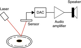
Compact discs [9] were first produced in Germany in 1982. Recorded voltage variations over time due to an acoustic sound is called an analog signal given its similarity with the differences in air pressure generated by the sound waves over time. Audio CDs and CD players illustrate best the conversion of a binary signal—unintelligible—into an intelligible analog signal. Moreover, the player is a very interesting control system.
To store an analog audio signal (e.g., voice or music) on a CD the signal must be first sampled and converted into a sequence of binary digits—a digital signal—by an ADC and then especially encoded to compress the information and to avoid errors when playing the CD. In the manufacturing of a CD, pits and bumps corresponding to the ones and zeros from the quantization and encoding processes are impressed on the surface of the disc. Such pits and bumps will be detected by the CD player and converted back into an analog signal that approximates the original signal when the CD is played. The transformation into an analog signal uses a DAC.
As we will see in Chapter 7, an audio signal is sampled at a rate of about 44,000 samples/second (sec) (corresponding to a maximum frequency around 22 KHz for a typical audio signal) and each of these samples is represented by a certain number of bits (typically 8 bits/sample). The need for stereo sound requires that two channels be recorded. Overall, the number of bits representing the signal is very large and needs to be compressed and especially encoded. The resulting data, in the form of pits and bumps impressed on the CD surface, are put into a spiral track that goes from the inside to the outside of the disc.
Besides the binary-to-analog conversion, the CD player exemplifies a very interesting control system (see Figure 0.2). Indeed, the player must: (1) rotate the disc at different speeds depending on the location of the track within the CD being read, (2) focus a laser and a lens system to read the pits and bumps on the disc, and (3) move the laser to follow the track being read. To understand the exactness required, consider that the width of the track and the high of the bumps is typically less than a micrometer (10−6 meters or 3.937 × 10⁻⁵ inches) and a nanometer (10−9 meters or 3.937 × 10⁻⁸ inches), respectively.
0.2.2. Software-Defined Radio and Cognitive Radio
Software-defined radio and cognitive radio are important emerging technologies in wireless communications [43]. In software-defined radio (SDR), some of the radio functions typically implemented in hardware are converted into software [64]. By providing smart processing to SDRs, cognitive radio (CR) will provide the flexibility needed to more efficiently use the radio frequency spectrum and to make available new services to users. In the United States the Federal Communication Commission (FCC), and likewise in other parts of the world the corresponding agencies, allocates the bands for different users of the radio spectrum (commercial radio and TV, amateur radio, police, etc.). Although most bands have been allocated, implying a scarcity of spectrum for new users, it has been found that locally at certain times of the day the allocated spectrum is not being fully utilized. Cognitive radio takes advantage of this.
Conventional radio systems are composed mostly of hardware, and as such cannot be easily reconfigured. The basic premise in SDR as a wireless communication system is its ability to reconfigure by changing the software used to implement functions typically done by hardware in a conventional radio. In an SDR transmitter, software is used to implement different types of modulation procedures, while ADCs and DACs are used to change from one type of signal to another. Antennas, audio amplifiers, and conventional radio hardware are used to process analog signals. Typically, an SDR receiver uses an ADC to change the analog signals from the antenna into digital signals that are processed using software on a general-purpose processor. See Figure 0.3.

Given the need for more efficient use of the radio spectrum, cognitive radio (CR) uses SDR technology while attempting to dynamically manage the radio spectrum. A cognitive radio monitors locally the radio spectrum to determine regions that are not occupied by their assigned users and transmits in those bands. If the primary user of a frequency band recommences transmission, the CR either moves to another frequency band, or stays in the same band but decreases its transmission power level or modulation scheme to avoid interference with the assigned user. Moreover, a CR will search for network services that it can offer to its users. Thus, SDR and CR are bound to change the way we communicate and use network services.
0.2.3. Computer-Controlled Systems
The application of computer control ranges from controlling simple systems such as a heater (e.g., keeping a room temperature comfortable while reducing energy consumption) or cars (e.g., controlling their speed), to that of controlling rather sophisticated machines such as airplanes (e.g., providing automatic flight control) or chemical processes in very large systems such as oil refineries. A significant advantage of computer control is the flexibility computers provide—rather sophisticated control schemes can be implemented in software and adapted for different control modes.
Typically, control systems are feedback systems where the dynamic response of a system is changed to make it follow a desirable behavior. As indicated in Figure 0.4, the plant is a system, such as a heater, car, or airplane, or a chemical process in need of some control action so that its output (it is also possible for a system to have several outputs) follows a reference signal (or signals). For instance, one could think of a cruise-control system in a car that attempts to keep the speed of the car at a certain value by controlling the gas pedal mechanism. The control action will attempt to have the output of the system follow the desired response, despite the presence of disturbances either in the plant (e.g., errors in the model used for the plant) or in the sensor (e.g., measurement error). By comparing the reference signal with the output of the sensor, and using a control law implemented in the computer, a control action is generated to change the state of the plant and attain the desired output.
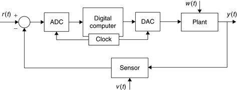
To use a computer in a control application it is necessary to transform analog signals into digital signals so that they can be inputted into the computer, while it is also necessary that the output of the computer be converted into an analog signal to drive an actuator (e.g., an electrical motor) to provide an action capable of changing the state of the plant. This can be done by means of ADCs and DACs. The sensor should also be able to act as a transducer whenever the output of the plant is of a different type than the reference. Such would be the case, for instance, if the plant output is a temperature while the reference signal is a voltage.
0.3. Analog or Discrete?
Infinitesimal calculus, or just plain calculus, deals with functions of one or more continuously changing variables. Based on the representation of these functions, the concepts of derivative and integral are developed to measure the rate of change of functions and the areas under the graphs of these functions, or their volumes. Differential equations are then introduced to characterize dynamic systems.
Finite calculus, on the other hand, deals with sequences. Thus, derivatives and integrals are replaced by differences and summations, while differential equations are replaced by difference equations. Finite calculus makes possible the computations of calculus by means of a combination of digital computers and numerical methods—thus, finite calculus becomes the more concrete mathematics. 1 Numerical methods applied to sequences permit us to approximate derivatives, integrals, and the solution of differential equations.
1The use of concrete, rather than abstract, mathematics was coined by Graham, Knuth, and Patashnik in Concrete Mathematics: A Foundation for Computer Science[26]. Professor Donald Knuth from Stanford University is the the inventor of the Tex and Metafont typesetting systems that are the precursors of Latex, the document layout system in which the original manuscript of this book was done.
In engineering, as in many areas of science, the inputs and outputs of electrical, mechanical, chemical, and biological processes are measured as functions of time with amplitudes expressed in terms of voltage, current, torque, pressure, etc. These functions are called analog or continuous-time signals, and to process them with a computer they must be converted into binary sequences—or a string of ones and zeros that is understood by the computer. Such a conversion is done in a way as to preserve as much as possible the information contained in the original signal. Once in binary form, signals can be processed using algorithms (coded procedures understood by computers and designed to obtain certain desired information from the signals or to change them) in a computer or in a dedicated piece of hardware.
In a digital computer, differentiation and integration can be done only approximately, and the solution of differential equations requires a discretization process as we will illustrate later in this chapter. Not all signals are functions of a continuous parameter—there exist inherently discrete-time signals that can be represented as sequences, converted into binary form, and processed by computers. For these signals the finite calculus is the natural way of representing and processing them.
Analog or continuous-time signals are converted into binary sequences by means of an ADC, which, as we will see, compresses the data by converting the continuous-time signal into a discrete-time signal or a sequence of samples, each sample being represented by a string of ones and zeros giving a binary signal. Both time and signal amplitude are made discrete in this process. Likewise, digital signals can be transformed into analog signals by means of a DAC that uses the reverse process of the ADC. These converters are commercially available, and it is important to learn how they work so that digital representation of analog signals is obtained with minimal information loss. Chapter 1, Chapter 7 and Chapter 8 will provide the necessary information about continuous-time and discrete-time signals, and show how to convert one into the other and back. The sampling theory presented in Chapter 7 is the backbone of digital signal processing.
0.3.1. Continuous-Time and Discrete-Time Representations
There are significant differences between continuous-time and discrete-time signals as well as in their processing. A discrete-time signal is a sequence of measurements typically made at uniform times, while the analog signal depends continuously on time. Thus, a discrete-time signal x[n] and the corresponding analog signal x(t) are related by a sampling process:
(0.1)
Clearly, by choosing a small value for Ts we could make the analog and the discrete-time signals look very similar—almost indistinguishable—which is good, but this is at the expense of memory space required to keep the numerous samples. If we make the value of Ts large, we improve the memory requirements, but at the risk of losing information contained in the original signal. For instance, consider a sinusoid obtained from a signal generator:

As indicated before, not all signals are analog; there are some that are naturally discrete. Figure 0.6 displays the weekly average of the stock price of a fictitious company, ACME. Thinking of it as a signal, it is naturally discrete-time as it does not come from the discretization of an analog signal.
 |
| Figure 0.6 |
We have shown in this section the significance of the sampling period Ts in the transformation of an analog signal into a discrete-time signal without losing information. Choosing the sampling period requires knowledge of the frequency content of the signal—this is an example of the relation between time and frequency to be presented in great detail in Chapter 4 and Chapter 5, where the Fourier representation of periodic and nonperiodic signals is given. In Chapter 7, where we consider the problem of sampling, we will use this relation to determine appropriate values for the sampling period.
0.3.2. Derivatives and Finite Differences
Differentiation is an operation that is approximated in finite calculus. The derivative operator
(0.2)
(0.3)
(0.4)
The forward finite-difference operator measures the difference between two consecutive samples: one in the future x((n + 1)Ts) and the other in the present x(nTs). (See Problem 0.4 for a definition of the backward finite-difference operator.) The symbols D and Δ are called operators as they operate on functions to give other functions. The derivative and the finite-difference operators are clearly not the same. In the limit, we have that
(0.5)
Intuitively, if a signal does not change very fast with respect to time, the finite-difference approximates well the derivative for relatively large values of Ts, but if the signal changes very fast one needs very small values of Ts. The concept of frequency of a signal can help us understand this. We will learn that the frequency content of a signal depends on how fast the signal varies with time; thus a constant signal has zero frequency while a noisy signal that changes rapidly has high frequencies. Consider a constant signal x0(t) = 2 having a derivative of zero (i.e., such a signal does not change at all with respect to time or it is a zero-frequency signal). If we convert this signal into a discrete-time signal using a sampling period Ts = 1 (or any other positive value), then x0[n] = 2 and so
It becomes clear that the faster the signal changes, the smaller the sampling period Ts should be in order to get a better approximation of the signal and its derivative. As we will learn in Chapter 4 and Chapter 5 the frequency content of a signal depends on the signal variation over time. A constant signal has frequency zero, while a signal that changes very fast over time would have high frequencies. The higher the frequencies in a signal, the more samples would be needed to represent it with no loss of information, thus requiring that Ts be smaller.
0.3.3. Integrals and Summations
Integration is the opposite of differentiation. To see this, suppose I(t) is the integration of a continuous signal x(t) from some time t0 to t(t0 < t),
(0.6)

2The integral I(t) is a function of t and as such the integrand needs to be expressed in terms of a so-called dummy variable τ that takes values from t0 to t in the integration. It would be confusing to let the integration variable be t. The variable τ is called a dummy variable because it is not crucial to the integration; any other variable could be used with no effect on the integration.
(0.7)

(0.8)
We will see in Chapter 3 a similar relation between the derivative and the integral. The Laplace transform operators s and 1/s (just like D and 1/D) imply differentiation and integration in the time domain.
Computationally, integration is implemented by sums. Consider, for instance, the integral of x(t) = t from 0 to 10, which we know is equal to


The approximation of the area using Ts = 1 is very poor (see Figure 0.7). In the above, we used the fact that the sum is not changed whether we add the numbers from 0 to 9 or backwards from 9 to 0, and that doubling the sum and dividing by 2 would not change the final answer. The above sum can thus be generalized to
(0.9)

3Carl Friedrich Gauss (1777–1855) was a German mathematician. He was seven years old when he amazed his teachers with his trick for adding the numbers from 1 to 100 [7]. Gauss is one of the most accomplished mathematicians of all times [2]. He is in a group of selected mathematicians and scientists whose pictures appear in the currency of a country. His picture was on the Mark, the previous currency of Germany [6].
 |
| Figure 0.7 |
To improve the approximation of the integral we use Ts = 10−3, which gives a discretized signal nTs for 0 ≤ nTs < 10 or 0 ≤ n ≤ (10/Ts) − 1. The area of the pulses is  and the approximation to the integral is then

Derivatives and integrals take us into the processing of signals by systems. Once a mathematical model for a dynamic system is obtained, typically differential equations characterize the relation between the input and output variable or variables of the system. A significant subclass of systems (used as a valid approximation in some way to actual systems) is given by linear differential equations with constant coefficients. The solution of these equations can be efficiently found by means of the Laplace transform, which converts them into algebraic equations that are much easier to solve. The Laplace transform is covered in Chapter 3, in part to facilitate the analysis of analog signals and systems early in the learning process, but also so that it can be related to the Fourier theory of Chapter 4 and Chapter 5. Likewise for the analysis of discrete-time signals and systems we present in Chapter 9 the Z-transform, having analogous properties to those from the Laplace transform, before the Fourier analysis of those signals and systems.
0.3.4. Differential and Difference Equations
A differential equation characterizes the dynamics of a continuous-time system, or the way the system responds to inputs over time. There are different types of differential equations, corresponding to different systems. Most systems are characterized by nonlinear, time-dependent coefficient differential equations. The analytic solution of these equations is rather complicated. To simplify the analysis, these equations are locally approximated as linear constant-coefficient differential equations.
Solution of differential equations can be obtained by means of analog and digital computers. An electronic analog computer consists of operational amplifiers (op-amps), resistors, capacitors, voltage sources, and relays. Using the linearized model of the op-amps, resistors, and capacitors it is possible to realize integrators to solve a differential equation. Relays are used to set the initial conditions on the capacitors, and the voltage source gives the input signal. Although this arrangement permits the solution of differential equations, its drawback is the storage of the solution, which can be seen with an oscilloscope but is difficult to record. Hybrid computers were suggested as a solution—the analog computer is assisted by a digital component that stores the data. Both analog and hybrid computers have gone the way of the dinosaurs, and it is digital computers aided by numerical methods that are used now to solve differential equations.
Before going into the numerical solution provided by digital computers, let us consider why integrators are needed in the solution of differential equations. A first-order (the highest derivative present in the equation); linear (no nonlinear functions of the input or the output are present) with constant-coefficient differential equations obtained from a simple RC circuit (Figure 0.8) with a constant voltage source vi(t) as input and with resistor R = 1Ω; and capacitor C = 1 F (with huge plates!) connected in series is given by
(0.10)
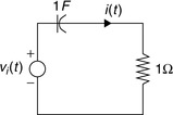
Intuitively, in this circuit the capacitor starts with an initial charge of vc(0), and will continue charging until it reaches saturation, at which point no more charge will flow (the current across the resistor and the capacitor is zero). Therefore, the voltage across the capacitor is equal to the voltage source–that is, the capacitor is acting as an open circuit given that the source is constant.
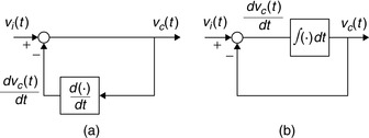
Suppose, ideally, that we have available devices that can perform differentiation. There is then the tendency to propose that the differential equation (Eq. 0.10) be solved following the block diagram shown in Figure (0.9). Although nothing is wrong analytically, the problem with this approach is that in practice most signals are noisy (each device produces electronic noise) and the noise present in the signal may cause large derivative values given its rapidly changing amplitudes. Thus, the realization of the differential equation using differentiators is prone to being very noisy (i.e., not good). Instead of, as proposed years ago by Lord Kelvin, 4 using differentiators we need to smooth out the process by using integrators, so that the voltage across the capacitor vc(t) is obtained by integrating both sides of Equation (0.10). Assuming that the source is switched on at time t = 0 and that the capacitor has an initial voltage vc(0), using the inverse relation between derivatives and integrals gives
4William Thomson, Lord Kelvin, proposed in 1876 the differential analyzer, a type of analog computer capable of solving differential equations of order 2 and higher. His brother James designed one of the first differential analyzers [78].
(0.11)
 |
| Figure 0.9 |
Block diagrams like the ones shown in Figure 0.9 allow us to visualize the system much better, and are commonly used. Integrators can be efficiently implemented using operational amplifiers with resistors and capacitors.
How to Obtain Difference Equations
Let us then show how Equation (0.10) can be solved using integration and its approximation, resulting in a difference equation. Using Equation (0.11) at t = t1 and t = t0 for t1 > t0, we have that


Assuming Δt = T, we then let t1 = nT and t0 = (n − 1)T. The above equation can be written as
(0.12)
(0.13)
The advantage of the difference equation is that it can be solved for increasing values of n using previously computed values of vc(nT), which is called a recursive solution. For instance, letting T = 10−3, vi(t) = 1, and defining M = 2T/(2 + T), K = (2 − T)/(2 + T), we obtain

5The infinite sum converges if  , which is satisfied in this case. If we multiply the sum by (1 − K) we get
 where we changed the variable in the second equation to
  . This explains why the sum is equal to 1/(1 − K).
Even though this is a very simple example, it clearly illustrates that very good approximations to the solution of differential equations can be obtained using numerical methods that are appropriate for implementation in digital computers.
The above example shows how to solve a differential equation using integration and approximation of the integrals to obtain a difference equation that a computer can easily solve. The integral approximation used above is the trapezoidal rule method, which is one among many numerical methods used to solve differential equations. Also we will see later that the above results in the bilinear transformation, which connects the Laplace s variable with the z variable of the Z-transform, and that will be used in Chapter 11 in the design of discrete filters.
0.4. Complex or Real?
Most of the theory of signals and systems is based on functions of a complex variable. Clearly, signals are functions of a real variable corresponding to time or space (if the signal is two-dimensional, like an image) so why would one need complex numbers in processing signals? As we will see later, time-dependent signals can be characterized by means of frequency and damping. These two characteristics are given by complex variables such as  (where σ is the damping factor and Ω is the frequency) in the representation of analog signals in the Laplace transform, or
  (where r is the damping factor and ω is the discrete frequency) in the representation of discrete-time signals in the Z-transform. Both of these transformations will be considered in detail in Chapter 3 and Chapter 9. The other reason for using complex variables is due to the response of systems to pure tones or sinusoids. We will see that such response is fundamental in the analysis and synthesis of signals and systems. We thus need a solid grasp of what is meant by complex variables and what a function of these is all about. In this section, complex variables will be connected to vectors and phasors (which are commonly used in the sinusoidal steady-state analysis of linear circuits).
0.4.1. Complex Numbers and Vectors
A complex number z represents any point (x, y) in a two-dimensional plane by z = x + jy, where  (real part of z) is the coordinate in the x axis and
  (imaginary part of z) is the coordinate in the y axis. The symbol
  just indicates that z needs to have two components to represent a point in the two-dimensional plane. Interestingly, a vector
  that emanates from the origin of the complex plane (0,0) to the point (x, y) with a length
(0.14)
(0.15)
It is important to understand that a rectangular plane or a polar complex plane are identical despite the different representation of each point in the plane. Furthermore, when adding or subtracting complex numbers the rectangular form is the appropriate one, while when multiplying or dividing complex numbers the polar form is more advantageous. Thus, if complex numbers  and
and  are added analytically, we obtain
Using their polar representations requires a geometric interpretation: the addition of vectors (see Figure 0.11). On the other hand, the multiplication of z and v is easily done using their polar forms as
 |
| Figure 0.11 |
One operation possible with complex numbers that is not possible with real numbers is complex conjugation. Given a complex number  its complex conjugate is
  —that is, we negate the imaginary part of z or reflect its angle. This operation gives that
(0.17)
0.4.2. Functions of a Complex Variable
Just like real-valued functions, functions of a complex variable can be defined. For instance, the logarithm of a complex number can be written as
It is important to mention that complex variables as well as functions of complex variables are more general than real variables and real-valued functions. The above definition of the logarithmic function is valid when z = x, with x a real value, and also when z = jy, a purely imaginary value. Likewise, the exponential function for z = x is a real-valued function.
Euler's Identity
One of the most famous equations of all times6 is
6A reader's poll done by Mathematical Intelligencer named Euler's identity the most beautiful equation in mathematics. Another poll by Physics World in 2004 named Euler's identity the greatest equation ever, together with Maxwell's equations. Paul Nahin's book Dr. Euler's Fabulous Formula (2006) is devoted to Euler's identity. It states that the identity sets “the gold standard for mathematical beauty”[73].
7Leonard Euler (1707–1783) was a Swiss mathematician and physicist, student of John Bernoulli, and advisor of Joseph Lagrange. We owe Euler the notation f(x) for functions, e for the base of natural logs,  , π for pi, Σ for sum, the finite difference notation Δ, and many more!
(0.18)
One way to verify this identity is to consider the polar representation of the complex number  , which has a unit magnitude since
  given the trigonometric identity
  . The angle of this complex number is
The relation between the complex exponentials and the sinusoidal functions is of great importance in signals and systems analysis. Using Euler's identity the cosine can be expressed as
(0.19)
(0.20)

These relations can be used to define the hyperbolic sinusoids as
(0.21)
(0.22)
(0.23)
Euler's identity can also be used to find different trigonometric identities. For instance,
0.4.3. Phasors and Sinusoidal Steady State
A sinusoid x(t) is a periodic signal represented by
(0.24)
8Heinrich Rudolf Hertz was a German physicist known for being the first to demonstrate the existence of electromagnetic radiation in 1888.
If one knows the frequency Ω0 (rad/sec) in Equation (0.24), the cosine is characterized by its amplitude and phase. This permits us to define phasors9 as complex numbers characterized by the amplitude and the phase of a cosine signal of a certain frequency Ω0. That is, for a voltage signal  the corresponding phasor is
9In 1883, Charles Proteus Steinmetz (1885–1923), German-American mathematician and engineer, introduced the concept of phasors for alternating current analysis. In 1902, Steinmetz became a professor of electrophysics at Union College in Schenectady, New York.
(0.25)
(0.26)
Interestingly enough, the angle ψ can be used to differentiate cosines and sines. For instance, when ψ = 0, the phasor V moving around at a rate of Ω0 generates as a projection on the real axis the voltage signal  , while when
  , the phasor V moving around again at a rate of Ω0 generates a sinusoid
  as it is projected onto the real axis. This establishes the well-known fact that the sine lags the cosine by π/2 radians or 90 degrees, or that the cosine leads the sine by π/2 radians or 90 degrees. Thus, the generation and relation of sines and cosines can be easily obtained using the plot in Figure 0.12.

Phasors can be related to vectors. A current source, for instance,

In Figure 0.13 we display the result of adding two phasors (frequency f0 = 20 Hz) and the sinusoid that is generated by the phasor  .
.


0.4.4. Phasor Connection
The fundamental property of a circuit made up of constant resistors, capacitors, and inductors is that its response to a sinusoid is also a sinusoid of the same frequency in steady state. The effect of the circuit on the input sinusoid is on its magnitude and phase and depends on the frequency of the input sinusoid. This is due to the linear and time-invariant nature of the circuit, and can be generalized to more complex continuous-time as well as discrete-time systems as we will see in Chapter 3, Chapter 4, Chapter 5, Chapter 9 and Chapter 10.
To illustrate the connection of phasors with dynamic systems consider a simple RC circuit (R = 1 Ω and C = 1 F). If the input to the circuit is a sinusoidal voltage source  and the voltage across the capacitor vc(t) is the output of interest, the circuit can be easily represented by the first-order differential equation

Comparing the steady-state response vc(t) with the input sinusoid vi(t), we see that they both have the same frequency Ω0, but the amplitude and phase of the input are changed by the circuit depending on the frequency Ω0. Since at each frequency the circuit responds differently, obtaining the frequency response of the circuit will be useful not only in analysis but in the design of circuits.
The sinusoidal steady-state is obtained using phasors. Expressing the steady-state response of the circuit as

The concepts of linearity and time invariance will be used in both continuous-time as well as discrete-time systems, along with the Fourier representation of signals in terms of sinusoids or complex exponentials, to simplify the analysis and to allow the design of systems. Thus, transform methods such as Laplace and the Z-transform will be used to solve differential and difference equations in an algebraic setup. Fourier representations will provide the frequency perspective. This is a general approach for both continuous-time and discrete-time signals and systems. The introduction of the concept of the transfer function will provide tools for the analysis as well as the design of linear time-invariant systems. The design of analog and discrete filters is the most important application of these concepts. We will look into this topic in Chapter 5, Chapter 6 and Chapter 11.
0.5. Soft Introduction to MATLAB
MATLAB is a computing language based on vectorial computations. 10 In this section, we will introduce you to the use of MATLAB for numerical and symbolic computations.
10MATLAB stands for matrix laboratory. MatWorks, the developer of MATLAB, was founded in 1984 by Jack Little, Steve Bangert, and Cleve Moler. Moler, a math professor at the University of New Mexico, developed the first version of MATLAB in Fortran in the late 1970s. It only had 80 functions and no M-files or toolboxes. Little and Bangert reprogrammed it in C and added M-files, toolboxes, and more powerful graphics [49].
0.5.1. Numerical Computations
The following instructions are intended for users who have no background in MATLAB but are interested in using it in signal processing. Once you get the basic information on how to use the language you will be able to progress on your own.
1. Create a directory where you will put your work, and from where you will start MATLAB. This is important because when executing a program, MATLAB will look at the current directory, and if the file is not present in the current directory, and if it is not a MATLAB function, MATLAB gives an error indicating that it cannot find the desired program.
2. There are two types of programs in MATLAB: the script, which consists in a list of commands using MATLAB functions or your own functions, and the functions, which are programs that can be called with different inputs and provide the corresponding outputs. We will show examples of both.
3. Once you start MATLAB, you will see three windows: the command window, where you will type commands; the command history, which keeps a list of commands that have been used; and the workspace, where the variables used are kept.
4. Your first command on the command window should be to change to your data directory where you will keep your work. You can do this in the command window by using the command CD (change directory) followed by the desired directory. It is also important to use the command clear all and clf to clear all previous variables in memory and all figures.
5. Help is available in several forms in MATLAB. Just type helpwin, helpdesk, or demo to get started. If you know the name of the function, help will give you the necessary information on the particular function, and it will also give you information on help itself. Use help to find more about the functions used in this introduction to MATLAB.
6. To type your scripts or functions you can use the editor provided by MATLAB; simply type edit. You can also use any text editor to create scripts or functions, which need to be saved with the .m extension.
Creating Vectors and Matrices
Comments are preceded by percent, and to begin a script, as the following, it is always a good idea to clear all previous variables and all previous figures.
% matlab primer
clear all% clear all variables
clf% clear all figures
% row and column vectors
x = [ 1 2 3 4]% row vector
y = x'% column vector
The corresponding output is as follows (notice that there is no semicolon (;) at the end of the lines to stop MATLAB from providing an output when the above script is executed).
x =
1234
1
2
3
4
To see the dimension of x and y variables, type
whos% provides information on existing variables
to which MATLAB responds
NameSizeBytes Class
x1x432 double array
y4x132 double array
Grand total is 8 elements using 64 bytes
Notice that a vector is thought of as a matrix; for instance, vector x is a matrix of one row and four columns. Another way to express the column vector y is the following, where each of the row terms is separated by a semicolon (;)
y = [1;2;3;4]% another way to write a column
To give as before:
y =
1
2
3
4
MATLAB does not allow arguments of vectors or matrices to be zero or negative. For instance, if we want the first entry of the vector y we need to type
y(1)% first entry of vector y
giving as output
ans =
1
If we type
y(0)
it will give us an error, to which we get the following warning:
??? Subscript indices must either be real positive integers or logicals.
MATLAB also has a peculiar way to provide information in a vector, for instance:
y(1:3)% first to third entry of column vector y
ans =
1
2
3
The following will give the third to the first entry in the row vector x (notice the difference in the two outputs; as expected the values of y are given in a column, while the requested entries of x are given in a row).
x(3:-1:1)% displays entries x(3) x(2) x(1)
Thus,
ans =
321
Matrices are constructed as an concatenation of rows (or columns):
A = [1 2; 3 4; 5 6]% matrix A with rows [1 2], [3 4] and [5 6]
A =
12
34
56
To create a vector corresponding to a sequence of numbers (in this case integers) there are different approaches, as follows:
n = 0:10% vector with entries 0 to 10 increased by 1
This approach gives the following as output:
n =
Columns 1 through 10
0123456789
Column 11
10
which is the same as the command
n = [0:10]
If we wish the increment different from 1 (default value), then we indicate it as in the following:
n1 = 0:2:10% vector with entries from 0 to 10 increased by 2
which gives
n1 =
0246810
We can combine the above vectors into one as follows:
nn1 = [n n1]% combination of vectors
nn1 =
Columns 1 through 10
0123456789
Columns 11 through 17
100246810
Vectorial Operations
MATLAB allows the conventional vectorial operations as well as facilitates others. For instance, if we wish to multiply by 3 every entry of the row vector x given above, the command
z = 3∗x% multiplication by a constant
would give
z =
36912
Besides the conventional multiplication of vectors with the correct dimensions, MATLAB allows two types of multiplications of one vector by another. The first one is where the entries of one vector are multiplied by the corresponding entries of the other. To effect this the two vectors should have the same dimension (i.e., both should be columns or rows with the same number of entries) and it is necessary to put a dot before the multiplication operator—that is, as shown here:
v = x.∗x% multiplication of entries of two vectors
v =
14916
The other type of multiplication is the conventional multiplication allowed in linear algebra. For instance, with that of a row vector by a column vector,
w = x∗x'% multiplication of x (row vector) by x'(column vector)
w = 30
the result is a constant—in this case, the length of the row vector should coincide with that of the column vector. If you multiply a column (say x’) of dimension 4 × 1 by a row (say x) of dimension 1 × 4 (notice that the 1s coincide at the end of the first dimension and at the beginning of the second), the multiplication  results in a 4 × 4 matrix.
The solution of a set of linear equations is very simple in MATLAB. To guarantee that a unique solution exists, the determinant of the matrix should be computed before inverting the matrix. If the determinant is zero MATLAB will indicate the solution is not possible.
% Solution of linear set of equations Ax = b
A = [1 0 0; 2 2 0; 3 3 3];% 3x3 matrix
t = det(A);% MATLAB function that calculates determinant
b = [2 2 2]';% column vector
x = inv(A)∗b;% MATLAB function that inverts a matrix
The results of these operations are not given because of the semicolons at the end of the commands. The following script could be used to display them:
disp(‘Ax = b’)% MATLAB function that displays the text in ‘ ’
A
b
x
t
which gives
Ax = b
A =
100
220
333
b =
2
2
2
x =
2.0000
−1.0000
−0.3333
t =
6
Another way to solve this set of equations is
x = b'/A'
Try it!
MATLAB provides a fast way to obtain certain vectors/matrices; for instance,
% special vectors and matrices
x = ones(1, 10)% row of ten 1s
x =
1111111111
A = ones(5, 5)% matrix of 5 x 5 1s
A =
11111
11111
11111
11111
11111
x1 = [x zeros(1, 5)]% vector with previous x and 5 0s
Columns 1 through 10
1111111111
Columns 11 through 15
00000
A(2:5, 2:5) = zeros(4, 4)% zeros in rows 2−5, columns 2−5
A =
11111
10000
10000
10000
10000
y = rand(1,10)% row vector with 10 random values (uniformly
% distributed in [0,1]
y =
Columns 1 through 6
0.95010.23110.60680.48600.89130.7621
Columns 7 through 10
0.45650.01850.82140.4447
Notice that these values are between 0 and 1. When using the normal or Gaussian-distributed noise the values can be positive or negative reals.
y1 = randn(1,10)% row vector with 10 random values
% (Gaussian distribution)
y1 =
Columns 1 through 6
−0.4326−1.66560.12530.2877−1.14651.1909
Columns 7 through 10
1.1892−0.03760.32730.1746
Using Built-In Functions and Creating Your Own
MATLAB provides a large number of built-in functions. The following script uses some of them.
% using built-in functions
t = 0:0.01:1;% time vector from 0 to 1 with interval of 0.01
x = cos(2∗pi∗t/0.1);% cos processes each of the entries in
% vector t to get the corresponding value in vector x
% plotting the function x
figure(1)% numbers the figure
plot(t, x)% interpolated continuous plot
xlabel(‘t (sec)’)% label of x-axis
ylabel(‘x(t)’)% label of y-axis
sound(1000∗x, 10000)
The results are given in Figure 0.14.
 |
| Figure 0.14 |
To learn about any of these functions use help. In particular, use help to learn about MATLAB routines for plotting plot and stem. Use help sound and help waveplay to learn about the sound routines available in MATLAB. Additional related functions are put at the end of these help files. Explore all of these and become aware of the capabilities of MATLAB. To illustrate the plotting and the sound routines, let us create a chirp that is a sinusoid for which the frequency is varying with time.
y = sin(2∗pi∗t.^2/.1);% notice the dot in the squaring
% t was defined before
sound(1000∗y, 10000)% to listen to the sinusoid
figure(2)% numbering of the figure
plot(t(1:100), y(1:100))% plotting of 100 values of y
figure(3)
plot(t(1:100), x(1:100), ‘k’, t(1:100), y(1:100), ‘r’)% plotting x and y on same plot
Let us hope you were able to hear the chirp, unless you thought it was your neighbor grunting. In this case, we plotted the first 100 values of t and y and let MATLAB choose the color for them. In the second plot we chose the colors: black (dashed lines) for x and blue (continuous line) for the second signal y(t) (see Figure 0.15).
 |
| Figure 0.15 |
Other built-in functions are sin, tan, acos, asin, atan, atan2, log, log10, exp, etc. Find out what each does using help and obtain a listing of all the functions in the signal processing toolbox.
You do not need to define π, as it is already done in MATLAB. For complex numbers also you do not need to define the square root of −1, which for engineers is ‘j’ and for mathematicians ‘i’ (they have no current to worry about).
% pi and j
pi
j
i
ans =
3.1416
ans =
0 + 1.0000i
ans =
0 + 1.0000i
Creating Your Own Functions
MATLAB has created a lot of functions to make our lives easier, and it allows us also to create—in the same way—our own. The following file is for a function f with an input of a scalar x and output of a scalar y related by a mathematical function:
function y = f(x)
y = x∗exp(−sin(x))/(1 + x^2);
Functions cannot be executed on their own—they need to be part of a script. If you try to execute the above function MATLAB will give the following:
??? format compact;function y = f(x)
|
Error: A function declaration cannot appear within a script M-file.
A function is created using the word “function” and then defining the output (y), the name of the function (f), and the input of the function (x), followed by lines of code defining the function, which in this case is given by the second line. In our function the input and the output are scalars. If you want vectors as input/output you need to do the computation in vectorial form—more later.
Once the function is created and saved (the name of the function followed by the extension .m), MATLAB will include it as a possible function that can be executed within a script. If we wish to compute the value of the function for x = 2 (f.m should be in the working directory) we proceed as follows:
x = 0:0.1:100;% create an input vector x
N = length(x);% find the length of x
y = zeros(1,N);% initialize the output y to zeros
for n = 1:N,% for the variable n from 1 to N, compute
y(n) = f(x(n));% the function
end
figure(3)
plot(x, y)
grid% put a grid on the figure
title(‘Function f(x)’)
xlabel(‘x’)
ylabel(‘y’)
This is not very efficient. A general rule in MATLAB is: Loops are to be avoided, and vectorial computations are encouraged. The results are shown in Figure 0.16.

The function working on a vector x, rather than one value, takes the following form (to make it different from the above function we let the denominator be 1 + x instead of 1 + x2):
function yy = ff(x)
% vectorial function
yy = x.∗exp(−sin(x))./(1 + x);
Again, this function must be in the working directory. Notice that the computation of yy is done considering x a vector; the .* and ./ are indicative of this. Thus, this function will accept a vector x and will give as output a vector yy, computed as indicated in the last line. When we use a function, the names of the variables used in the script that calls the function do not need to coincide with the ones in the definition of the function. Consider the following script:
z = ff(x);% x defined before,
% z instead of yy is the output of the function ff
figure(4)
plot(x, z); grid
title(‘Function ff(x)’) % MATLAB function that puts title in plot
xlabel(‘x’) % MATLAB function to label x-axis
ylabel(‘z’) % MATLAB function to label y-axis
The difference between plot and stem is important. The function plot interpolates the vector to be plotted and so the plot appears continuous, while stem simply plots the entries of the vector, separating them uniformly. The input x and the output of the function are discrete time and we wish to plot them as such, so we use stem.
stem(x(1:30), z(1:30))
grid
title(‘Function ff(x)’)
xlabel(‘x’)
ylabel(‘z’)
The results are shown in Figure 0.17.


More on Plotting
There are situations where we want to plot several plots together. One can superpose two or more plots by using hold on and hold off. To put several figures in the same plot, we can use the function subplot. Suppose we wish to plot four figures in one plot and they could be arranged as two rows of two figures each. We do the following:
subplot(221)
plot(x, y)
subplot(222)
plot(x, z)
subplot(223)
stem(x, y)
subplot(224)
stem(x, z)
In the subplot function the first two numbers indicate the number of rows and the number of columns, and the last digit refers to the order of the graph that is, 1, 2, 3, and 4 (see Figure 0.18).

There is also a way to control the values in the axis, by using the function (you guessed!) axis. This function is especially useful after we have a graph and want to improve its looks. For instance, suppose that the professor would like the above graphs to have the same scales in the y-axis (picky professor). You notice that there are two scales in the y-axis, one 0-0.8 and another 0-3. To have both with the same scale, we choose the one 0-3, and modify the above code to the following
subplot(221)
plot(x, y)
axis([0 100 0 3])
subplot(222)
plot(x, z)
axis([0 100 0 3])
subplot(223)
stem(x, y)
subplot(224)
stem(x, z)
axis([0 100 0 3])
Saving and Loading Data
In many situations you would like to either save some data or load some data. The following is one way to do it. Suppose you want to build and save a table of sine values for angles between 0 and 360 degrees in intervals of 3 degrees. This can be done as follows:
x = 0:3:360;
y = sin(x∗pi/180); % sine computes the argument in radians
xy = [x' y']; % vector with 2 columns one for x'
% and another for y'
Let's now save these values in a file “sine.mat” by using the function save (use help save to learn more):
save sine.mat xy
To load the table, we use the function load with the name given to the saved table “sine” (the extension *.mat is not needed). The following script illustrates this:
clear all
load sine
whos
NameSizeBytesClass
xy121x21936double array
Grand total is 242 elements using 1936 bytes
This indicates that the array xy has 121 rows and 2 columns, the first colum corresponding to x, the degree values, and the second column corresponding to the sine values, y. Verify this and plot the values by using
x = xy(:, 1);
y = xy(:, 2);
stem(x, y)
Finally, MATLAB provides some data files for experimentation and you only need to load them. The following “train.mat” is the recording of a train whistle, sampled at the rate of Fs samples/sec, which accompanies the sampled signal y(n) (see Figure 0.19).

clear all
load train
whos
NameSizeBytesClass
Fs1x18double array
y12880x1103040double array
Grand total is 12881 elements using 103048 bytes
sound(y, Fs)
plot(y)
MATLAB also provides two-dimensional signals, or images, such as “clown.mat,” a 200 × 320 pixels image.
clear all
load clown
whos
NameSizeBytesClass
X200x320512000double array
caption2x14char array
map81x31944double array
Grand total is 64245 elements using 513948 bytes
We can display this image in gray levels by using the following script (see Figure 0.20):

colormap(‘gray’)
imagesc(X)
Or in color using
colormap(‘hot’)
imagesc(X)
0.5.2. Symbolic Computations
We have considered the numerical capabilities of MATLAB, by which numerical data are transformed into numerical data. There will be many situations when we would like to do algebraic or calculus operations resulting in terms of variables rather than numerical data. For instance, we might want to find a formula to solve quadratic algebraic equations, to find a difficult integral, or to obtain the Laplace or the Fourier transform of a signal. For those cases MATLAB provides the Symbolic Math Toolbox a symbolic computing system. In this section, we provide you with an introduction to symbolic computations by means of examples, and hope to get you interested in learning more on your own.
Derivatives and Differences
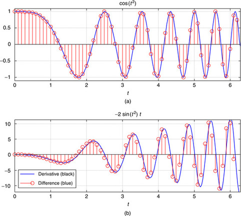
The following script compares symbolic with numeric computations of the derivative of a chirp signal (a sinusoid with changing frequency)  , which is
clf; clear all
% symbolic
syms t y z % define the symbolic variables
y = cos(t^2) % chirp signal -- notice no . before ^ since t is no vector
z = diff(y) % derivative
figure(1)
subplot(211)
ezplot(y, [0, 2∗pi]);grid % plotting for symbolic y between 0 and 2∗pi
hold on
subplot(212)
ezplot(z, [0, 2∗pi]);grid
hold on
%numeric
Ts = 0.1; % sampling period
t1 = 0:Ts:2∗pi; % sampled time
y1 = cos(t1.^2); % sampled signal --notice difference with y above
z1 = diff(y1)./diff(t1); % difference -- approximation to derivative
figure(1)
subplot(211)
stem(t1, y1, ‘r’);axis([0 2∗pi 1.1∗min(y1) 1.1∗max(y1)])
subplot(212)
stem(t1(1:length(y1) - 1), z1, ‘r’);axis([0 2∗pi 1.1∗min(z1) 1.1∗max(z1)])
legend(‘Derivative (black)’,‘Difference (blue)’)
hold off
The symbolic function syms defines the symbolic variables (use help syms to learn more). The signal y(t) is written differently than y1(t) in the numeric computation. Since t1 is a vector, squaring it requires a dot before the symbol. That is not the case for t, which is not a vector but a variable. The results of using diff to compute the derivative of y(t) is given in the same form as you would have obtained doing the derivative by hand—that is,
y = cos(t^2)
z = −2∗t∗sin(t^2)
The symbolic toolbox provides its own graphic routines (use help to learn about the different ez-routines). For plotting y(t) and z(t), we use the function ezplot, which plots the above two functions for  and titles the plots with these functions.
The numeric computations differ from the symbolic in that vectors are being processed, and we are obtaining an approximation to the derivative z(t). We sample the signal with Ts = 0.1 and use again the function diff to approximate the derivative (the denominator diff(t1) is the same as Ts). Plotting the exact derivative (continuous line) with the approximated one (samples) using stem clarifies that the numeric computation is an approximation at nTs values of time. See Figure 0.21.
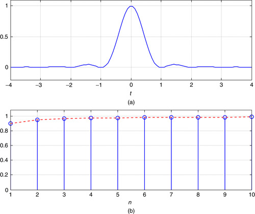
The Sinc Function and Integration
The sinc function is very significant in the theory of signals and systems. It is defined as
 |
| Figure 0.22 |
clf; clear all
% symbolic
syms t z
for k = 1:10,
zz(k) = subs(2∗z);% substitution to numeric value zz
end
% numeric
t1 = linspace(−4, 4);% 100 equally spaced points in [-4,4]
y = sinc(t1).^2;% numeric definition of the squared sinc function
n = 1:10;
figure(1)
subplot(211)
plot(t1, y);grid;axis([−4 4 −0.2 1.1∗max(y)]);title(‘y(t)=sinc^2(t)’);
xlabel(‘t’)
subplot(212)
stem(n(1:10), zz(1:10)); hold on
plot(n(1:10), zz(1:10), ‘r’);grid;title(‘∫ y(τ) dτ’); hold off
axis([1 10 0 1.1*max(zz)]); xlabel(‘n’)
Figure 0.22 shows the squared sinc function and the values of the integral
Chebyshev Polynomials and Lissajous Figures
The Chebyshev polynomials are used in the design of filters. They can be obtained by plotting two cosine functions as they change with time t, one of fix frequency and the other with increasing frequency:
 |
| Figure 0.23 |
syms x y t
x = cos(2∗pi∗t); theta=0;
figure(1)
for k = 1:4,
y = cos(2∗pi∗k∗t + theta);
if k == 1, subplot(221)
elseif k == 2, subplot(222)
elseif k == 3, subplot(223)
else subplot(224)
end
ezplot(x, y);grid;hold on
end
hold off
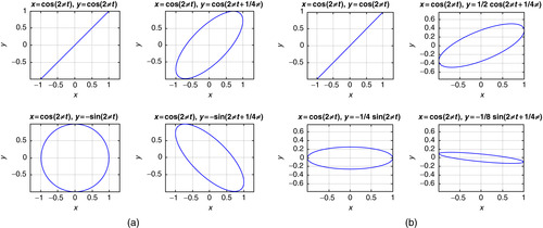
The Lissajous figures we consider next are a very useful extension of the above plotting of sinusoids in the x and y axes. These figures are used to determine the difference between a sinusoidal input and its corresponding sinusoidal steady state. In the case of linear systems, which we will formally define in Chapter 2, for a sinusoidal input the outputs of the system are also sinusoids of the same frequency, but they differ with the input in the amplitude and phase.
The differences in amplitude and phase can be measured using an oscilloscope for which we put the input in the horizontal sweep and the output in the vertical sweep, giving figures from which we can find the differences in amplitude and phase. Two situations are simulated in the following script, one where there is no change in amplitude but the phase changes from zero to 3π/4, while in the other case the amplitude decreases as indicated and the phase changes in the same way as before. The plots, or Lissajous figures, indicate such changes. The difference between the maximum and the minimum of each of the figures in the x axis gives the amplitude of the input, while the difference between the maximum and the minimum in the y axis gives the amplitude of the output. The orientation of the ellipse provides the difference in phase with respect to that of the input. The following script is used to obtain the Lissajous figures in these cases. Figure 0.24 displays the results.
 |
| Figure 0.24 |
clear all;clf
syms x y t
x = cos(2∗pi∗t); % input of unit amplitude and frequency 2*pi
A = 1;figure(1)% amplitude of output in case 1
for i = 1:2,
for k = 0:3,
y = A^k∗cos(2∗pi∗t + theta);
if k == 0,subplot(221)
elseif k == 1,subplot(222)
elseif k == 2,subplot(223)
else subplot(224)
end
ezplot(x, y);grid;hold on
end
A = 0.5; figure(2) % amplitude of output in case 2
end
Ramp, Unit-Step, and Impulse Responses
To close this introduction to symbolic computations we illustrate the response of a linear system represented by a differential equation,
 |
| Figure 0.25 |
clear all; clf
syms y t x z
% input a unit-step (heaviside) response
y = dsolve(‘D2y + 5*Dy + 6∗y = heaviside(t)’,‘y(0) = 0’,‘Dy(0) = 0’,‘t’);
x = diff(y); % impulse response
z = int(y); % ramp response
figure(1)
subplot(311)
ezplot(y, [0,5]);title(‘Unit-step response’)
subplot(312)
ezplot(x, [0,5]);title(‘Impulse response’)
subplot(313)
ezplot(z, [0,5]);title(‘Ramp response’)
This example illustrates the intuitive appeal of linear systems. When the input is a constant value (or a unit-step signal or a heaviside signal) the output tries to follow the input after some initial inertia and it ends up being constant. The impulse signal (obtained as the derivative of the unit-step signal) is a signal of very short duration equivalent to shocking the system with a signal that disappears very fast, different from the unit-step signal that is like a dc source. Again the output tries to follow the input, eventually disappearing as t increases (no energy from the input!), and the ramp that is the integral of the unit-step signal grows with time, providing more and more energy to the system as time increases, thus the response we obtained. The function dsolve solves differential equations explicitly given (D stands for the derivative operator, so D is the first derivative and D2 is the second derivative). A second-order system requires two initial conditions, the output and its derivative at t = 0.
We hope this introduction to MATLAB has provided you with the necessary background to understand the basic way MATLAB operates, and shown you how to continue increasing your knowledge of it. Your best source of information is the help command. Explore the different modules that MATLAB has and you will become quickly convinced that these modules provide a great number of computational tools for many areas of engineering and mathematics. Try it—you will like it! Table 0.1 and Table 0.2 provide a listing of the numeric and symbolic variables and operations.
For the problems requiring implementation in MATLAB, write scripts or functions to solve them numerically or symbolically. Label the axes of the plots, give a title, and use legend to identify different signals in a plot. To save space use subplot to put several plots into one. To do the problem numerically, sample analog signals with a small Ts.
Bits or Bytes
Just to get an idea of the number of bits or bytes generated and processed by a digital system consider the following applications:
(a) A compact disc is capable of storing 75 minutes of “CD-quality” stereo (left and right channels are recorded) music. Calculate the number of bytes and the number of bits that are stored in the CD. Hint: Find out what “CD quality” means in the binary representation of each sample, and what is the sampling rate your CD player uses.
(b) Find out what the vocoder in your cell phone is used for. Assume then that in attaining “telephone quality” you use a sampling rate of 10,000 samples/sec to achieve that type of voice quality. Each sample is represented by 8 bits. With this information, calculate the number of bits that your cell phone has to process every second that you talk. Why would you then need a vocoder?
(c) Find out whether text messaging is cheaper or more expensive than voice. Explain how text messaging works.
(d) Find out how an audio CD and an audio DVD compare. Find out why it is said that a vinyl long play record reproduces sounds much better. Are we going backwards with digital technology in music recording? Explain.
(e) To understand why video streaming in the Internet is many times of low quality, consider the amount of data that need to be processed by a video compressor every second. Assume the size of a video frame, in picture elements or pixels, is 352 × 240, and that an acceptable quality for the image is obtained by allocating 8 bits/pixel, and to avoid jerking effects we use 60 frames/sec.
■ How many pixels would have to be processed every second?
■ How many bits would be available for transmission every second?
■ The above are raw data. Compression changes the whole picture (literally); find out what some of the compression methods are.
Sampling—MATLAB
Consider an analog signal x(t) = 4 cos(2π t) defined for −∞ < t < ∞. For the following values of the sampling period Ts, generate a discrete-time signal  .
.
■ Ts = 0.1 sec
■ Ts = 0.5 sec
■ Ts = 1 sec
Determine for which values of Ts the discrete-time signal has lost the information in the analog signal. Use MATLAB to plot the analog signal (use the plot function) and the resulting discrete-time signals (use the stem function). Superimpose the analog and the discrete-time signals for 0 ≤ t ≤ 3; use subplot to plot the four figures as one figure. For plotting the analog signal use Ts = 10−4. You also need to figure out how to label the different axes and have the same scales and units. In Chapter 7 on sampling we will show how to reconstruct sampled signals.
Derivative and Finite Difference—MATLAB
Let y(t) = dx(t)/dt, where x(t) is the signal in Problem 0.2. Find y(t) analytically and determine a value of Ts for which  (consider Ts = 0.01 and Ts = 0.1). Use the MATLAB function diff or create your own to compute the finite difference. Plot the finite difference in the range [0,1] and compare it with the actual derivative y(t) in that range. Explain your results for the given values of Ts.
Backward Difference—MATLAB
 (
( approximates the derivative of x(t).)
(a) Indicate how this new definition connects with the finite difference defined earlier in this chapter.
(b) Solve Problem 0.3 with MATLAB using this new finite difference and compare your results with the ones obtained there.
(c) For the value of Ts = 0.1, use the average of the two finite differences to approximate the derivative of the analog signal x(t). Compare this result with the previous ones. Provide an expression for calculating this new finite difference directly.
Differential and Difference Equations—MATLAB
Find the differential equation relating a current source  with the current iL(t) in an inductor, with inductance L = 1 H, connected in parallel with a resistor of R = 1 Ω (see Figure 0.26). Assume a zero initial current in the inductor.
 |
| Figure 0.26 Problem 0.5. RL circuit: input is(t) and output iL(t). |
(a) Obtain a discrete equation from the differential equation using the trapezoidal approximation of an integral.
(b) Create a MATLAB script to solve the difference equation for Ts = 0.01 and three frequencies for is(t), Ω0 = 0.005π, 0.05π, and 0.5π. Plot the input current source is(t) and the approximate solution iL(nTs) in the same figure. Use the MATLAB function plot. Use the MATLAB function filter to solve the difference equation (use help to learn about filter).
(c) Solve the differential equation using symbolic MATLAB when the input frequency is Ω0 = 0.5π.
(d) Use phasors to find the amplitude of iL(t) when the input is is(t) with the given three frequencies.
Sums and Gauss—MATLAB
 and similarly for
  . Let c be a constant, and choose any permutation of the values [0,1,2] for instance [2,1,0] or [1,0,2].
 To do so, consider
 and apply the above rules to find S.
 for constants α and β, using the given three rules.
Three rules in the computation of sums are
(a) Explain why the above rules make sense when computing sums. To do that consider
(b) The trick that Gauss played when he was a preschooler can be explained by using the above rules. Suppose you want to find the sum of the integers from 0 to 10000 (Gauss did it for integers between 0 and 100 but he was then just a little boy, and we can do better!). That is, we want to find S where
(c) Find the sum of an arithmetic progression
(d) Find out if MATLAB can do these sums symbolically (i.e., without having numerical values).
Integrals and Sums—MATLAB

Suppose you wish to find the area under a signal using sums. You will need the following result found above:
(a) Consider first x(t) = t, 0 ≤ t ≤ 1, and zero otherwise. The area under this signal is 0.5. The integral can be approximated from above and below as
(b) Let Ts = 0.001. Use the symbolic function symsum to compute the left and right bounds for the above integral. Find the average of these results and compare it with the actual value of the integral.
(c) Verify the symbolic results by finding the sums on the left and the right of the above inequality using the summation given at the beginning of the problem. You need to change the dummy variables.
(d) Write a similar MATLAB script to compute the area under the signal y(t) = t2 from 0 ≤ t ≤ 1. Let Ts = 0.001. Compare the average of the lower and upper bounds to the value of the integral.
Integrals and Sums—MATLAB
 Show that this is true by computing the three integrals. Then consider the sum
 Find this sum and determine which of the following is equal to this sum:
 Use symbolic MATLAB function symsum to verify your answers.
Although sums behave like integrals, because of the discrete nature of sums one needs to be careful with the upper and lower limits more than in the integral case. To illustrate this, consider the separation of an integral into two integrals and compare them with the separation of a sum into two sums. For the integral we have that
Sum of Geometric Series
 will be used quite frequently in the next chapters, so let us look at some of its properties:
 This can be done by showing that
  . Why do you need the constraint that α ≠ 1? Would this sum exist if α > 1? Explain.
 Obtain an expression to find S1.
The geometric series
(a) Suppose α = 1; what is S equal to?
(b) Suppose α ≠ 1; show that
(d) Suppose now that N = ∞; under what conditions will S exist? If it does, what would S be equal to? Explain.
(e) Suppose the derivative of S with respect to α is
Exponentials—MATLAB
The exponential  for t ≥ 0 and zero otherwise is a very common analog signal. Likewise,
  for integers n ≥ 0 and zero otherwise is a very common discrete-time signal. Let us see how they are related. Do the following using MATLAB:
(a) Let a = −0.5; plot x(t).
(b) Let a = −1; plot the corresponding signal x(t). Does this signal go to zero faster than the exponential for a = −0.5?
(c) Suppose we sample the signal x(t) using Ts = 1; what would be x(nTs) and how can it be related to y(n) (i.e., what is the value of α that would make the two equal)?
(d) Suppose that a current  for t ≥ 0 and zero otherwise is applied to a discharged capacitor of capacitance C = 1 F at t = 0. What would be the voltage in the capacitor at t = 1 sec?
(e) How would you obtain an approximate result to the above problem using a computer? Explain.
Algebra of Complex Numbers
Consider complex numbers  , and
, and  .
.
(a) In the complex plane, indicate the point (x, y) that corresponds to z and then show a vector  that joins the point (x, y) to the origin. What is the magnitude and the angle corresponding to z or
  ?
?
(b) Do the same for the complex numbers w, v, and u. Plot the four complex numbers and find their sum z + w + v + u analytically and graphically.
(c) Find the ratios z/w, w/v, and u/z. Determine the real and imaginary parts of each, as well as their magnitudes and phases. Using the ratios find u/w.
(d) The phase of a complex number is only significant when the magnitude of the complex number is significant. Consider z and y = 10−16z; compare their magnitudes and phases. What would you say about the phase of y?
Algebra of Complex Numbers

Consider a function of z = 1 + j1,
(a) Find log(w).
(b) Find the real and the imaginary parts of w.
(c) What is  , where
  is the complex conjugate of w?
(d) Determine |w|, ∠w.
(e) What is |log(w)|2?
(f) Express cos(1) in terms of w using Euler's equation.
Euler's Identity and Trigonometric Identities
Use Euler's identity to obtain an expression for  ; obtain its real and imaginary components and show the following identities:
■ cos(α + β) = cos(α) cos(β) − sin(α) sin(β)
■ sin(α + β) = sin(α) cos(β) + sin(β) cos(α)
Hint: Find real and imaginary parts of  and of
  .
.
Euler's Identity and Trigonometric Identities
Algebra of Complex Numbers

 is the magnitude of z and
 is the angle or phase of z. Thus, whenever we are multiplying or dividing complex numbers the polar form is more appropriate.
 On the other hand, when showing that
  the polar form is more appropriate.
 Find the polar forms of z and w and then find zw by using the rectangular and then the polar forms and decide which is easier. As a bonus you should get the trigonometric identities for cos(θ + ϕ) and sin(θ + ϕ). What are they?
(a) The complex conjugate of z = x + jy is  . Using these rectangular representations, show that
(b) Show that it is easier to find the above results by using the polar representation  of z where
(c) Whenever we are adding or subtracting complex numbers the rectangular representation is more appropriate. Show that for two complex numbers z = x + jy and w = v + jq; then,
(d) If the above conclusions still do not convince you, consider then the case of multiplying two complex numbers:
Vectors and Complex Numbers
 Show it geometrically by representing z as a vector.
 Show a geometric example that verifies this.
Using the vectorial representation of complex numbers it is possible to get some interesting inequalities:
(a) Is it true that for a complex number z = x + jy:
(b) The so-called triangle inequality says that for any complex (or real) numbers z and v we have that
Complex Functions of Time—MATLAB


Consider the complex function  for −∞ < t < ∞.
(a) Find the real and the imaginary parts of x(t) and carefully plot them with MATLAB. Try to make MATLAB plot x(t) directly. What do you get? Does MATLAB warn you? Does it make sense?
(c) Compute the integral
(d) Would the following statement be true (remember * indicates complex conjugate)?
Euler's Equation and Orthogonality of Sinusoids
 is very useful not only in obtaining the rectangular and polar forms of complex numbers, but in many other respects as we will explore in this problem.
 Use Euler's equation to express the sines in terms of exponentials, multiply the resulting exponentials, and use Euler's equation to regroup the expression in terms of sinusoids.
 For instance, consider x(t) = cos(π t) and y(t) = sin(π t). Check first that these functions repeat every T0 = 2 (i.e., show that x(t + 2) = x(t) and that y(t + 2) = y(t)). Thus, T0 = 2 can be seen as their period. Then use the representation of a cosine in terms of complex exponentials,
 to express the integrand in terms of exponentials and calculate the integral.
Euler's equation,
(a) Carefully plot  for −∞ < n < ∞. Is this a real or a complex signal?
(b) Suppose you want to find the trigonometric identity corresponding to
(c) As we will see later on, two periodic signals x(t) and y(t) of period T0 are said to be orthogonal if the integral over a period T0 is
Euler's Equation and Trigonometric Expressions

Obtain using Euler's equation an expression for sin(θ) in terms of exponentials and then
(a) Use it to obtain the trigonometric identity for sin2(θ).
(b) Compute the integral
De Moivre's Theorem for Roots
 where N ≥ 1 is an integer and
  a nonzero complex number.
 where
where  and θk = (ϕ + 2π k)/N for k = 0, 1, …, N − 1.
 and plot them in a polar plane (i.e., indicating their magnitude and phase).
(a) First verify that there are exactly N roots of this equation and that they are given by
(b) Use the above result to find the roots of the following equations:
(c) Explain how the roots are distributed around a circle of radius r in the complex polar plane.
Natural Log of Complex Numbers
 If z is negative it can be written as
  and we can find log(z) by using the above derivation. The log of any complex number can be obtained this way also.
Suppose you want to find the log of a complex number  . Its logarithm can be found to be
(a) Justify each one of the steps in the above equation.
(b) Find
Hyperbolic Sinusoids—MATLAB
 Let x = jθ and find cos(x). The resulting function is called the hyperbolic cosine or
In filter design you will be asked to use hyperbolic functions. In this problem we relate these functions to sinusoids and obtain a definition of these functions so that we can actually plot them.
(a) Consider computing the cosine of an imaginary number—that is, use
(b) Consider then the computation of the hyperbolic sine sinh(θ); how would you do it? Carefully plot it as a function of θ.
(d) Show that sinh(θ) = −sinh(−θ).
(e) Write a MATLAB script to compute and plot these functions between −10 and 10.
Phasors!
 How much is this shift Δt? Better yet, what is Δθ = Ω0Δt or the shift in phase? One thus only need to consider cosine functions with different phase shifts instead of sines and cosines.
A phasor can be thought of as a vector, representing a complex number, rotating around the polar plane at a certain frequency expressed in radians/sec. The projection of such a vector onto the real axis gives a cosine. This problem will show the algebra of phasors, which would help you with some of the trigonometric identities that are hard to remember.
(a) When you plot a sine signal y(t) = A sin(Ω0t), you notice that it is a cosine x(t) = A cos(Ω0t) shifted in time—that is,
(b) You should have found the answer above is Δθ = π/2 (if not, go back and try it and see if it works). Thus, the phasor that generates x(t) = A cos(Ω0t) is  so that
  . The phasor corresponding to the sine y(t) should then be
  . Obtain an expression for y(t) similar to the one for x(t) in terms of this phasor.
(c) According to the above results, give the phasors corresponding to −x(t) = −A cos(Ω0t) and −y(t) = −sin(Ω0t). Plot the phasors that generate cos, sin, −cos, and −sin for a given frequency. Do you see now how these functions are connected? How many radians do you need to shift in a positive or negative direction to get a sine from a cosine, etc.
(d) Suppose then you have the sum of two sinusoids, for instance z(t) = x(t) + y(t), adding the corresponding phasors for x(t) and y(t) at some time (e.g., t = 0), which is just a sum of two vectors, you should get a vector and the corresponding phasor. Get the phasor for z(t) and the expression for it in terms of a cosine.
..................Content has been hidden....................
You can't read the all page of ebook, please click here login for view all page.