
Chapter 6. Application to Control and Communications
Who are you going to believe? Me or your own eyes.
Julius “Groucho” Marx (1890–1977) comedian and actor
6.1. Introduction
Control and communications are areas in electrical engineering where the Laplace and the Fourier analyses apply. In this chapter, we illustrate how these transform methods and the concepts of transfer function, frequency response, and spectrum connect with the classical theories of control and communications.
In classical control, the objective is to change the dynamics of a given system to be able to achieve a desired response by frequency-domain methods. This is typically done by means of a feedback connection of a controller to a plant. The plant is a system such as a motor, a chemical plant, or an automobile we would like to control so that it responds in a certain way. The controller is a system we design to make the plant follow a prescribed input or reference signal. By feeding back the response of the system to the input, it can be determined how the plant responds to the controller. The commonly used negative feedback generates an error signal that permits us to judge the performance of the controller. The concepts of transfer function, stability of systems, and different types of responses obtained through the Laplace transform are very useful in the analysis and design of classical control systems.
A communication system consists of three components: a transmitter, a channel, and a receiver. The objective of communications is to transmit a message over a channel to a receiver. The message is a signal, for instance, a voice or a music signal, typically containing low frequencies. Transmission of the message can be done over the airwaves or through a line connecting the transmitter to the receiver, or a combination of the two—constituting channels with different characteristics. Telephone communication can be done with or without wires, and radio and television are wireless. The concepts of frequency, bandwidth, spectrum, and modulation developed by means of the Fourier transform are fundamental in the analysis and design of communication systems.
The aim of this chapter is to serve as an introduction to problems in classical control and communications and to link them with the Laplace and Fourier analyses. More in-depth discussion of these topics can be found in many excellent texts in control and communications.
The other topic covered in this chapter is an introduction to analog filter design. Filtering is a very important application of LTI systems in communications, control, and digital signal processing. The material in this chapter will be complemented by the design of discrete filters in Chapter 11. Important issues related to signals and system are illustrated in the design and implementation of filters.
6.2. System Connections and Block Diagrams
Control and communication systems consist of interconnection of several subsystems. As we indicated in Chapter 2, there are three important connections of LTI systems:
■ Cascade
■ Parallel
■ Feedback
Cascade and parallel result from properties of the convolution integral, while the feedback connection relates the output of the overall system to its input. With the background of the Laplace transform we present now a transform characterization of these connections that can be related to the time-domain characterizations given in Chapter 2.
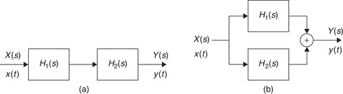
The connection of two LTI continuous-time systems with transfer functions H1(s) and H2(s) (and corresponding impulse responses h1(t) and h2(t)) can be done in:
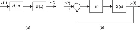
■ Cascade (Figure 6.1(a)): Provided that the two systems are isolated, the transfer function of the overall system is
(6.1)
■ Parallel (Figure 6.1(b)): The transfer function of the overall system is
(6.2)
■ Negative feedback (Figure 6.4): The transfer function of the overall system is
(6.3)
■ Open-loop transfer function:  .
.
■ Closed-loop transfer function:  .
.
 |
| Figure 6.1 |
Cascading of LTI Systems
Given two LTI systems with transfer functions  and
and  where h1(t) and h2(t) are the corresponding impulse responses of the systems, the cascading of these systems gives a new system with transfer function
■ It requires isolation of the systems.
■ It causes delay as it processes the input signal, possibly compounding any errors in the processing.
Remarks
■ Loading, or lack of system isolation, needs to be considered when cascading two systems. Loading does not allow the overall transfer function to be the product of the transfer functions of the connected systems. Consider the cascade connection of two resistive voltage dividers (Figure 6.2), each with a simple transfer function Hi(s) = 1/2, i = 1, 2. The cascade inFigure 6.2(b)clearly will not have as transfer function H(s) = H1(s)H2(s) = (1/2)(1/2) unless we include a buffer (such as an operational amplifier voltagefollower) in between (seeFigure 6.2(a)). The cascading of the two voltage dividers without the voltage follower gives a transfer function H1(s) = 1/5, as can be easily shown by doing mesh analysis on the circuit.
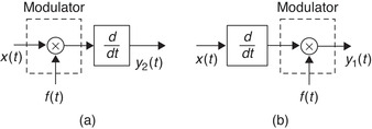
■ The block diagrams of the cascade of two or more LTI systems can be interchanged with no effect on the overall transfer function, provided the connection is done with no loading. That is not true if the systems are not LTI. For instance, consider cascading a modulator (LTV system) and a differentiator (LTI) as shown inFigure 6.3. If the modulator is first,Figure 6.3(a), the output of the overall system is
 |
| Figure 6.2 |
Parallel Connection of LTI Systems
According to the distributive property of the convolution integral, the parallel connection of two or more LTI systems has the same input and its output is the sum of the outputs of the systems being connected (see Figure 6.1(b)). The parallel connection is better than the cascade, as it does not require isolation between the systems, and reduces the delay in processing an input signal. The transfer function of the parallel system is
Remarks
■ Although a communication system can be visualized as the cascading of three subsystems—the transmitter, the channel, and the receiver—typically none of these subsystems is LTI. As we discussed inChapter 5, the low-frequency nature of the message signals requires us to use as the transmitter a system that can generate a signal with much higher frequencies, and that is not possible with LTI systems (recall the eigenfunction property). Transmitters are thus typically nonlinear or linear time varying. The receiver is also not LTI. A wireless channel is typically time varying.
■ Some communication systems use parallel connections (see quadrature amplitude modulation (QAM) later in this chapter). To make it possible for several users to communicate over the same channel, a combination of parallel and cascade connections are used (see frequency division multiplexing (FDM) systems later in this chapter). But again, it should be emphasized that these subsystems are not LTI.
Feedback Connection of LTI Systems
In control, feedback connections are more appropriate than cascade or parallel connections. In the feedback connection, the output of the first system is fed back through the second system into the input (see Figure 6.4). In this case, like in the parallel connection, beside the blocks representing the systems we use adders to add/subtract two signals.
 |
| Figure 6.4 |
It is possible to have positive- or negative-feedback systems depending on whether we add or subtract the signal being fed back to the input. Typically, negative feedback is used, as positive feedback can greatly increase the gain of the system. (Think of the screeching sound created by an open microphone near a loud-speaker: the microphone continuously picks up the amplified sound from the loud-speaker, increasing the volume of the produced signal. This is caused by positive feedback.) For negative feedback, the connection of two systems is done by putting one in the feedforward loop, H1(s), and the other in the feedback loop, H2(s) (there are other possible connections). To find the overall transfer function we consider the Laplace transforms of the error signal e(t), E(s), and of the output y(t), Y(s), in terms of the Laplace transform of the input x(t), X(s), and the transfer functions H1(s) and H2(s) of the systems:

(6.4)
6.3. Application to Classic Control
Because of different approaches, the theory of control systems can be divided into classic and modern control. Classic control uses frequency-domain methods, while modern control uses time-domain methods. In classic linear control, the transfer function of the plant we wish to control is available; let us call it G(s). The controller, with a transfer function Hc(s), is designed to make the output of the overall system perform in a specified way. For instance, in a cruise control the plant is the car, and the desired performance is to automatically set the speed of the car to a desired value. There are two possible ways the controller and the plant are connected: in open-loop or in closed-loop (see Figure 6.5).
 |
| Figure 6.5 |
Open-Loop Control
In the open-loop approach the controller is cascaded with the plant (Figure 6.5(b)). To make the output y(t) follow the reference signal at the input x(t), we minimize an error signal
Remarks
Although open-loop systems are simple to implement, they have several disadvantages:
■ The controller Hc(s) must cancel the poles and the zeros of G(s) exactly, which is not very practical. In actual systems, the exact location of poles and zeros is not known due to measurement errors.
■ If the plant G(s) has zeros on the right-hand s-plane, then the controller Hc(s) will be unstable, as its poles are the zeros of the plant.
■ Due to ambiguity in the modeling of the plant, measurement errors, or simply the presence of noise, the output y(t) is typically affected by a disturbance signal η(t) mentioned above (η(t) is typically random—we are going to assume for simplicity that it is deterministic so we can compute its Laplace transform).The Laplace transform of the overall system output is
Closed-Loop Control
Assuming y(t) and x(t) in the open-loop control are the same type of signals, (e.g., both are voltages, or temperatures), if we feed back y(t) and compare it with the input x(t) we obtain a closed-loop control. Considering the case of negative-feedback system (see Figure 6.5(a)), and assuming no disturbance (η(t) = 0), we have that

If a disturbance signal η(t) (consider it for simplicity deterministic and with Laplace transform η(s)) is present (See Figure 6.5(a)), the above analysis becomes

Remarks
A control system includes two very important components:
■ Transducer: Since it is possible that the output signal y(t) and the reference signal x(t) might not be of the same type, a transducer is used to change the output so as to be compatible with the reference input. Simple examples of a transducer are: lightbulbs, which convert voltage into light; a thermocouple, which converts temperature into voltage.
■ Actuator: A device that makes possible the execution of the control action on the plant, so that the output of the plant follows the reference input.
Controlling an Unstable Plant
Consider a dc motor modeled as an LTI system with a transfer function

Suppose then that X(s) = 1/s2 or that x(t) = tu(t), a ramp signal. Intuitively, this is a much harder situation to control, as the output needs to be continuously growing to try to follow the input. In this case, the Laplace transform of the error signal is
Choosing the values of the gain K of the open-loop transfer function
A Cruise Control
Suppose we are interested in controlling the speed of a car or in obtaining a cruise control. How to choose the appropriate controller is not clear. We consider initially a proportional plus integral (PI) controller Hc(s) = 1 + 1/s and will ask you to consider the proportional controller as an exercise. See Figure 6.7.

Suppose we want to keep the speed of the car at V0 miles/hour for t ≥ 0 (i.e., x(t) = V0u(t)), and that the model for a car in motion is a system with transfer function


6.3.1. Stability and Stabilization
A very important question related to the performance of systems is: How do we know that a given causal system has finite zero-input, zero-state, or steady-state responses? This is the stability problem of great interest in control. Thus, if the system is represented by a linear differential equation with constant coefficients the stability of the system determines that the zero-input, the zero-state, as well as the steady-state responses may exist. The stability of the system is also required when considering the frequency response in the Fourier analysis. It is important to understand that only the Laplace transform allows us to characterize stable as well as unstable systems; the Fourier transform does not.
Two possible ways to look at the stability of a causal LTI system are:
■ When there is no input so that the response of the system depends on initial energy in the system. This is related to the zero-input response of the system.
■ When there is a bounded input and no initial condition. This is related to the zero-state response of the system.
Relating the zero-input response of a causal LTI system to stability leads to asymptotic stability. An LTI system is said to be asymptotically stable if the zero-input response (due only to initial conditions in the system) goes to zero as t increases—that is,
(6.5)
The second interpretation leads to the bounded-input bounded-output (BIBO) stability, which we defined in Chapter 2. A causal LTI system is BIBO stable if its response to a bounded input is also bounded. The condition we found in Chapter 2 for a causal LTI system to be BIBO stable was that the impulse response of the system be absolutely integrable—that is
(6.6)

Consider a system being represented by the differential equation


A causal LTI system with transfer function H(s) = B(s)/A(s) exhibiting no pole-zero cancellation is said to be:
■ Asymptotically stable if the all-pole transfer function H1(s) = 1/A(s), used to determine the zero-input response, has all its poles in the open left-hand s-plane (the jΩ axis excluded), or equivalently
(6.7)
■ BIBO stable if all the poles of H(s) are in the open left-hand s-plane (the jΩ axis excluded), or equivalently
(6.8)
■ If H(s) exhibits pole-zero cancellations, the system can be BIBO stable but not necessarily asymptotically stable.
Testing the stability of a causal LTI system thus requires finding the location of the roots of A(s), or the poles of the system. This can be done for low-order polynomials A(s) for which there are formulas to find the roots of a polynomial exactly. But as shown by Abel, 1 there are no equations to find the roots of higher than fourth-order polynomials. Numerical methods to find roots of these polynomials only provide approximate results that might not be good enough for cases where the poles are close to the jΩ axis. The Routh stability criterion [53] is an algebraic test capable of determining whether the roots of A(s) are on the left-hand s-plane or not, thus determining the stability of the system.
1Niels H. Abel (1802–1829) was a Norwegian mathematician who accomplished brilliant work in his short lifetime. At age 19, he showed there is no general algebraic solution for the roots of equations of degree greater than four, in terms of explicit algebraic operations.
Stabilization of a Plant
Consider a plant with a transfer function G(s) = 1/(s − 2), which has a pole in the right-hand s-plane and therefore is unstable. Let us consider stabilizing it by cascading it with an all-pass filter (Figure 6.8(a)) so that the overall system is not only stable but also keeps its magnitude response. To get rid of the pole at s = 2 and to replace it with a new pole at s = −2, we let the all-pass filter be


 |
| Figure 6.8 |
Consider then a negative-feedback system (Figure 6.8(b)). Suppose we use a proportional controller with a gain K, then the overall system transfer function is
6.3.2. Transient Analysis of First- and Second-Order Control Systems
Although the input to a control system is not known a-priori, there are many applications where the system is frequently subjected to a certain type of input and thus one can select a test signal. For instance, if a system is subjected to intense and sudden inputs, then an impulse signal might be the appropriate test input for the system; if the input applied to a system is constant or continuously increasing, then a unit step or a ramp signal would be appropriate. Using test signals such as an impulse, a unit-step, a ramp, or a sinusoid, mathematical and experimental analyses of systems can be done.
When designing a control system its stability becomes its most important attribute, but there are other system characteristics that need to be considered. The transient behavior of the system, for instance, needs to be stressed in the design. Typically, as we drive the system to reach a desired response, the system's response goes through a transient before reaching the desired response. Thus, how fast the system responds and what steady-state error it reaches need to be part of the design considerations.
First-Order Systems
As an example of a first-order system consider an RC serial circuit with a voltage source vi(t) = u(t) as input (Figure 6.9), and as the output the voltage across the capacitor, vc(t). By voltage division, the transfer function of the circuit is

 |
| Figure 6.10 |
%%%%%%%%%%%%%%%%%%%%%
% Transient analysis
%%%%%%%%%%%%%%%%%%%%%
clf; clear all
syms s t
num = [0 1];
for RC = 1:2:10,
den = [RC 1];
figure(1)
splane(num, den) % plotting of poles and zeros
hold on
vc = ilaplace(1/(RC ∗ s^2 + s)) % inverse Laplace
figure(2)
ezplot(vc, [0, 50]); axis([0 50 0 1.2]); grid
hold on
end
hold off
Second-Order System
A series RLC circuit with the input a voltage source, vs(t), and the output the voltage across the capacitor, vc(t), has a transfer function
(6.9)
(6.10)
(6.11)


Indeed, the transfer function of the feedback system is given by

Assume Ωn = 1 rad/sec and let 0 ≤ ψ ≤ 1 (so that the poles of H(s) are complex conjugate for 0 ≤ ψ < 1 and double real for ψ = 1). Let the input be a unit-step signal so that Vs(s) = 1/s. We then have:
(a) If we plot the poles of H(s) as ψ changes from 0 (poles in jΩ axis) to 1 (double real poles) the response y(t) in the steady state changes from a sinusoid shifted up by 1 to a damped signal. The locus of the poles is a semicircle of radius Ωn = 1. Figure 6.12 shows this behavior of the poles and the responses.
(b) As in the first-order system, the location of the poles determines the response of the system. The system is useless if the poles are on the jΩ axis, as the response is completely oscillatory and the input will never be followed. On the other extreme, the response of the system is slow when the poles become real. The designer would have to choose a value in between these two for ψ.
(c) For values of ψ between  to 1 the oscillation is minimum and the response is relatively fast (see Figure 6.12(b)). For values of ψ from 0 to
  the response oscillates more and more, giving a large steady-state error (see Figure 6.12(c)).
 |
| Figure 6.12 |
In this example we find the response of an LTI system to different inputs by using functions in the control toolbox of MATLAB. You can learn more about the capabilities of this toolbox, or set of specialized functions for control, by running the demo respdemo and then using help to learn more about the functions tf, impulse, step, and pzmap, which we will use here.
We want to create a MATLAB function that has as inputs the coefficients of the numerator N(s) and of the denominator D(s) of the system's transfer function H(s) = N(s)/D(s) (the coefficients are ordered from the highest order to the lowest order or constant term). The other input of the function is the type of response t where t = 1 corresponds to the impulse response, t = 2 to the unit-step response, and t = 3 to the response to a ramp. The output of the function is the desired response. The function should show the transfer function, the poles, and zeros, and plot the corresponding response. We need to figure out how to compute the ramp response using the step function.
Consider the following transfer functions:
(a) 
(b) 
Solution
The following script is used to look at the desired responses of the two systems and the location of their poles and zeros. We consider the second system; you can run the script for the first system by putting % at the numerator and the denominator after H2(s) and getting rid of % after H1(s) in the script. The function response computes the desired responses (in this case the impulse, step, and ramp responses).
%%%%%%%%%%%%%%%%%%%
% Example 6.4 -- Control toolbox
%%%%%%%%%%%%%%%%%%%
clear all; clf
% % H_1(s)
% nu = [1 1]; de = [1 1 1];
%% H_2(s)
nu = [1 0]; de = [1 1 1 1]; % unstable
h = response(nu, de, 1);
s = response(nu, de, 2);
r = response(nu, de, 3);
function y = response(N, D, t)
sys = tf(N, D)
poles = roots(D)
zeros = roots(N)
figure(1)
pzmap(sys);grid
if t == 3,
D1 = [D 0]; % for ramp response
end
figure(2)
if t == 1,
subplot(311)
y = impulse(sys,20);
plot(y);title(’ Impulse response’);ylabel(’h(t)’);xlabel(’t’); grid
elseif t == 2,
subplot(312)
y = step(sys, 20);
plot(y);title(’ Unit-step response’);ylabel(’s(t)’);xlabe(’t’);grid
else
subplot(313)
sys = tf(N, D1); % ramp response
y = step(sys, 40);
plot(y); title(’ Ramp response’); ylabel(’q(t)’); xlabel(’t’);grid
end
The results for H2(s) are as follows.
Transfer function:
s
-----------------------
s^3 + s^2 + s + 1
poles =
−1.0000
−0.0000 + 1.0000i
−0.0000 − 1.0000i
zeros =
0
As you can see, two of the poles are on the jΩ axis, and so the system corresponding to H2(s) is unstable. The other system is stable. Results for both systems are shown in Figure 6.13.

6.4. Application to Communications
The application of the Fourier transform in communications is clear. The representation of signals in the frequency domain and the concept of modulation are basic in communications. In this section we show examples of linear (amplitude modulation or AM) as well as nonlinear (frequency modulation or FM, and phase modulation or PM) modulation methods. We also consider important extensions such as frequency-division multiplexing (FDM) and quadrature amplitude modulation (QAM).
Given the low-pass nature of most message signals, it is necessary to shift in frequency the spectrum of the message to avoid using a very large antenna. This can be attained by means of modulation, which is done by changing either the magnitude or the phase of a carrier:
(6.12)
6.4.1. AM with Suppressed Carrier
Consider a message signal m(t) (e.g., voice or music, or a combination of the two) modulating a cosine carrier cos(Ωct) to give an amplitude modulated signal
(6.13)
(6.14)

At the receiver, we need to first detect the desired signal among the many signals transmitted by several sources. This is possible with a tunable band-pass filter that selects the desired signal and rejects the others. Suppose that the signal obtained by the receiver, after the band-pass filtering, is exactly s(t)—we then need to demodulate this signal to get the original message signal m(t). This is done by multiplying s(t) by a cosine of exactly the same frequency of the carrier in the transmitter (i.e., Ωc), which will give r(t) = 2s(t) cos(Ωct), which again according to the modulation property has a Fourier transform
(6.15)
The above is a simplification of the actual processing of the received signal. Besides the many other transmitted signals that the receiver encounters, there is channel noise caused by interferences from equipment in the transmission path and interference from other signals being transmitted around the carrier frequency. This noise will also be picked up by the band-pass filter and a perfect recovery of m(t) will not be possible. Furthermore, the sent signal has no indication of the carrier frequency Ωc, which is suppressed in the sent signal, and so the receiver needs to guess it and any deviation would give errors.
Remarks
■ The transmitter is linear but time varying. AM-SC is thus called a linear modulation. The fact that the modulated signal displays frequencies much higher than those in the message indicates the transmitter is not LTI—otherwise it would satisfy the eigenfunction property.
■ A more general characterization than Ωc >> 2πf0where f0is the largest frequency in the message is given by Ωc >> BW where BW (rad/sec) is the bandwidth of the message. You probably recall the definition of bandwidth of filters used in circuit theory. In communications there are several possible definitions for bandwidth. The bandwidth of a signal is the width of the range of positive frequencies for which some measure of the spectral content is satisfied. For instance, two possible definitions are:
■ The half-power or 3-dB bandwidth is the width of the range of positive frequencies where a peak value at zero or infinite frequency (low-pass and high-pass signals) or at a center frequency (band-pass signals) is attenuated to 0.707, the value at the peak. This corresponds to the frequencies for which the power at dc, infinity, or center frequency reduces to half.
■ The null-to-null bandwidth determines the width of the range of positive frequencies of the spectrum of a signal that has a main lobe containing a significant part of the energy of the signal. If a low-pass signal has a clearly defined maximum frequency, then the bandwidth are frequencies from zero to the maximum frequency, and if the signal is a band-pass signal and has a minimum and a maximum frequency, its bandwidth is the maximum minus the minimum frequency.
■ In AM-SC demodulation it is important to know exactly the carrier frequency. Any small deviation would cause errors when recovering the message. Suppose, for instance, that there is a small error in the carrier frequency—that is, instead of Ωcthe demodulator uses Ωc + Δ—so that the received signal in that case has the Fourier transform

6.4.2. Commercial AM
In commercial broadcasting, the carrier is added to the AM signal so that information of the carrier is available at the receiver helping in the identification of the radio station. For demodulation, such information is not important, as commercial AM uses envelope detectors to obtain the message. By making the envelope of the modulated signal look like the message, detecting this envelope is all that is needed. Thus, the commercial AM signal is of the form
Remarks
■ The advantage of adding the carrier to the message, which allows the use of a simple envelope detector, comes at the expense of increasing the power in the transmitted signal.
■ The demodulation in commercial AM is called noncoherent. Coherent demodulation consists in multiplying—or mixing—the received signal with a sinusoid of the same frequency and phase of the carrier. A local oscillator generates this sinusoid.
■ A disadvantage of commercial as well as suppressed-carrier AM is the doubling of the bandwidth of the transmitted signal compared to the bandwidth of the message. Given the symmetry of the spectrum, in magnitude as well as in phase, it becomes clear that it is not necessary to send the upper and the lower sidebands of the spectrum to get back the signal in the demodulation. It is thus possible to have upper- and lower-sideband AM modulations, which are more efficient in spectrum utilization.
■ Most AM receivers use the superheterodyne receiver technique developed by Armstrong and Fessenden.2
2Reginald Fessenden was the first to suggest the heterodyne principle: mixing the radio-frequency signal using a local oscillator of different frequency, resulting in a signal that could drive the diaphragm of an earpiece at an audio frequency. Fessenden could not make a practical success of the heterodyne receiver, which was accomplished by Edwin H. Armstrong in the 1920s using electron tubes.
Simulation of AM modulation with MATLAB
For simulations, MATLAB provides different data files, such as “train.mat” (the extension mat indicates it is a data file) used here. Suppose the analog signal y(t) is a recording of a “choo-choo” train, and we wish to use it to modulate a cosine cos(Ωct) to create an amplitude modulated signal z(t). Because the train y(t) signal is given in a sampled form, the simulation requires discrete-time processing, and so we will comment on the results here and leave the discussion of the issues related to the code for the next chapters.
The carrier frequency is chosen to be fc = 20.48 KHz. For the envelope detector to work at the transmitter we add a constant K to the message to ensure this sum is positive. The envelope of the AM-modulated signal should resemble the message. Thus, the AM signal is

6.4.3. AM Single Sideband
The message m(t) is typically a real-valued signal that, as indicated before, has a symmetric spectrum—that is, the magnitude and the phase of the Fourier transform M(Ω) are even and odd functions of frequency. When using AM modulation the resulting spectrum has redundant information by providing the upper and the lower sidebands. To reduce the bandwidth of the transmitted signal, we could get rid of either the upper or the lower sideband of the AM signal. The resulting modulation is called AM single sideband (AM-SSB) (upper or lower sideband depending on which of the two sidebands is kept). This type of modulation is used whenever the quality of the received signal is not as important as the advantages of a narrowband and having less noise in the frequency band of the received signal. AM-SSB is used by amateur radio operators.
As shown in Figure 6.16, the upper sideband modulated signal is obtained by band-pass filtering the upper sideband in the modulated signal. At the receiver, band-pass filtering the received signal the output is then demodulated like in an AM-SC system, and the result is then low-pass filtered using the bandwidth of the message.

6.4.4. Quadrature AM and Frequency-Division Multiplexing
Quadrature amplitude modulation (QAM) and frequency division multiplexing (FDM) are the precursors of many of the new communication systems. QAM and FDM are of great interest for their efficient use of the radio spectrum.
Quadrature Amplitude Modulation
QAM enables two AM-SC signals to be transmitted over the same frequency band, conserving bandwidth. The messages can be separated at the receiver. This is accomplished by using two orthogonal carriers, such as a cosine and a sine (see Figure 6.17). The QAM-modulated signal is given by
(6.16)
 |
| Figure 6.17 |
To simplify the computation of the spectrum of s(t), let us consider the message m(t) = m1(t) − jm2(t) (i.e., a complex message) with spectrum M(Ω) = M1(Ω) − jM2(Ω) so that

Frequency-Division Multiplexing
Frequency-division multiplexing (FDM) implements sharing of the spectrum by several users by allocating a specific frequency band to each. One could, for instance, think of the commercial AM or FM locally as an FDM sytem. In the United States, the Federal Communication Commission (FCC) is in charge of the spectral allocation. In telephony, using a bank of filters it is possible to also get several users in the same system—it is, however, necessary to have a similar system at the receiver to have a two-way communication.
To illustrate an FDM system (Figure 6.18), consider we have a set of messages of known finite bandwidth (we could low-pass filter the messages to satisfy this condition) that we wish to transmit. Each of the messages modulate different carriers so that the modulated signals are in different frequency bands without interfering with each other (if needed a frequency guard could be used to make sure of this). These frequency-multiplexed messages can now be transmitted. At the receiver, using a bank of band-pass filters centered at the carrier frequencies in the transmitter and followed by appropriate demodulators recover the different messages (see FDM receiver in Figure 6.18). Any of the AM modulation techniques could be used in the FDM system.

6.4.5. Angle Modulation
Amplitude modulation is said to be linear modulation, because as a system it behaves like a linear system. Frequency and phase, or angle, modulation systems on the other hand are nonlinear. The interest in angle modulation is due to the decreasing effect of noise or interferences on it, when compared with AM, although at the cost of a much wider bandwidth and greater complexity in implementation. The nonlinear behavior of angle modulation systems makes their analysis more difficult than that for AM. The spectrum of an FM or PM signal is much harder to obtain than that of an AM signal. In the following we consider the case of the so-called narrowband FM where we are able to find its spectrum directly.
Professor Edwin H. Armstrong developed the first successful frequency modulation system—narrowband FM. 3 If m(t) is the message signal, and we modulate a carrier signal of frequency Ωc (rad/sec) with m(t), the transmitted signal s(t) in angle modulation is of the form
3Edwind H. Armstrong (1890–1954), professor of electrical engineering at Columbia University, and inventor of some of the basic electronic circuits underlying all modern radio, radar, and television, was born in New York. His inventions and developments form the backbone of radio communications as we know it.
(6.17)
(6.18)
(6.19)
(6.20)
(6.21)
(6.22)
In amplitude modulation the bandwidth depends on the frequency of the message, while in frequency modulation the bandwidth depends on the amplitude of the message.
Thus, the modulated signals are
(6.23)
(6.24)
Narrowband FM
In this case the angle θ(t) is small, so that cos(θ(t)) ≈ 1 and sin(θ(t)) ≈ θ(t), simplifying the spectrum of the transmitted signal:

(6.26)
(6.27)
Simulation of FM modulation with MATLAB
In these simulations we will concern ourselves with the results and leave the discussion of issues related to the code for the next chapter since the signals are approximated by discrete-time signals. For the narrowband FM we consider a sinusoidal message
 |
| Figure 6.19 |
To illustrate the wideband FM, we consider two messages,


6.5. Analog Filtering
The basic idea of filtering is to get rid of frequency components of a signal that are not desirable. Application of filtering can be found in control, in communications, and in signal processing. In this section we provide a short introduction to the design of analog filters. Chapter 11 is dedicated to the design of discrete filters and to some degree that chapter will be based on the material in this section.
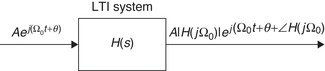
According to the eigenfunction property of LTI systems (Figure 6.21) the steady-state response of an LTI system to a sinusoidal input—with a certain magnitude, frequency, and phase—is a sinusoid of the same frequency as the input, but with magnitude and phase affected by the response of the system at the frequency of the input. Since periodic as well as aperiodic signals have Fourier representations consisting of sinusoids of different frequencies, the frequency components of any signal can be modified by appropriately choosing the frequency response of the LTI system, or filter. Filtering can thus be seen as a way of changing the frequency content of an input signal.
The appropriate filter for a certain application is specified using the spectral characterization of the input and the desired spectral characteristics of the output. Once the specifications of the filter are set, the problem becomes one of approximation as a ratio of polynomials in s. The classical approach in filter design is to consider low-pass prototypes, with normalized frequency and magnitude responses, which may be transformed into other filters with the desired frequency response. Thus, a great deal of effort is put into designing low-pass filters and into developing frequency transformations to map low-pass filters into other types of filters. Using cascade and parallel connections of filters also provide a way to obtain different types of filters.
The resulting filter should be causal, stable, and have real-valued coefficients so that it can be used in real-time applications and realized as a passive or an active filter. Resistors, capacitors, and inductors are used in the realization of passive filters, while resistors, capacitors, and operational amplifiers are used in active filter realizations.
6.5.1. Filtering Basics
A filter H(s) = B(s)/A(s) is an LTI system having a specific frequency response. The convolution property of the Fourier transform gives that
(6.28)
Magnitude Squared Function
The magnitude-squared function of an analog low-pass filter has the general form
(6.29)
■ Selection of the appropriate function f(.).
■ The factorization needed to get H(s) from the magnitude-squared function.
As an example of the above steps, consider the Butterworth low-pass analog filter. The Butterworth magnitude-squared response of order N is
(6.30)
(6.31)
Filter Specifications
Although an ideal low-pass filter is not realizable (recall the Paley-Wiener condition in Chapter 5) its magnitude response can be used as prototype for specifying low-pass filters. Thus, the desired magnitude is specified as
(6.32)
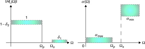
To simplify the computation of the filter parameters, and to provide a scale that has more resolution and physiological significance than the specifications given above, the magnitude specifications are typically expressed in a logarithmic scale. Defining the loss function (in decibels, or dBs) as
(6.33)
(6.34)
In the above specifications, the dc loss was 0 dB corresponding to a normalized dc gain of 1. In more general cases, α(0) ≠ 0 and the loss specifications are given as α(0) = α1, α2 in the passband and α3 in the stopband. To normalize these specifications we need to subtract α1, so that the loss specifications are

The design problem is then: Given the magnitude specifications in the passband (α(0), αmax, and Ωp) and in the stopband (αmin and Ωs) we then
1. Choose the rational approximation method (e.g., Butterworth).
2. Solve for the parameters of the filter to obtain a magnitude-squared function that satisfies the given specifications.
6.5.2. Butterworth Low-Pass Filter Design
The magnitude-squared approximation of a low-pass N th-order Butterworth filter is given by
(6.35)
Remarks
■ The half-power frequency is called the −3-dB frequency because in the case of the low-pass filter with a dc gain of 1, at the half-power frequency Ωhpthe magnitude-squared function is
(6.36)
(6.37)
■ It is important to understand the significance of the frequency and magnitude normalizations typical in filter design. Having a low-pass filter with normalized magnitude, its dc gain is 1, if one desires a filter with a DC gain K ≠ 1 it can be obtained by multiplying the magnitude-normalized filter by the constant K. Likewise, a filter H(S) designed with a normalized frequency, say Ω′ = Ω/Ωhpso that the normalized half-power frequency is 1, is converted into a denormalized filter H(s) with a desired Ωhpby replacing S = s/Ωhpin H(S).
Factorization
To obtain a filter that satisfies the specifications and that is stable we need to factorize the magnitude-squared function. By letting S = s/Ωhp be a normalized Laplace variable, then S/j = Ω′ = Ω/Ωhp and
(6.38)
(6.39)
Remarks
■ Since |Sk| = 1, the poles of the Butterworth filter are on a circle of unit radius. De Moivre's theorem guarantees that the poles are also symmetrically distributed around the circle, and because of the condition that complex poles should be complex conjugate pairs, the poles are symmetrically distributed with respect to the σ axis. Letting S = s/Ωhpbe the normalized Laplace variable, then s = SΩhp, so that the denormalized filter H(s) has its poles in a circle of radius Ωhp.
■ No poles are on the jΩ′ axis, as can be seen by showing that the angle of the poles are not equal to π/2 or 3π/2. In fact, for 1 ≤ k ≤ N, the angle of the poles are bounded below and above by letting 1 ≤ k and then k ≤ N to get
■ Consecutive poles are separated by π/N radians from each other. In fact, subtracting the angles of two consecutive poles can be shown to give ±π/N.
Using the above remarks and the fact that the poles must be in conjugate pairs, since the coefficients of the filter are real-valued, it is easy to determine the location of the poles geometrically.
A second-order low-pass Butterworth filter, normalized in magnitude and in frequency, has a transfer function of
The DC gain of H(S) is unity—in fact, when Ω = 0, S = j0 gives H(j0) = 1. The half-power frequency of H(S) is unity, indeed letting Ω′ = 1, then S = j1 and
Thus, the desired filter with a dc gain of 10 is obtained by multiplying H(S) by 10. Furthermore, if we let S = s/100 be the normalized Laplace variable when  , we get that s = jΩhp = j100, or Ωhp = 100, the desired half-power frequency. Thus, the denormalized filter in frequency H(s) is obtained by replacing S = s/100. The denormalized filter in magnitude and frequency is then

Design
For the Butterworth low-pass filter, the design consists in finding the parameters N, the minimum order, and Ωhp, the half-power frequency, of the filter from the constrains in the passband and in the stopband.
The loss function for the low-pass Butterworth is
(6.40)
(6.42)
(6.43)
Remarks
■ According toEquation (6.43)when either
■ The transition band is narrowed (i.e., Ωp → Ωs), or
■ The loss αminis increased, or
■ The loss αmaxis decreased
■ The minimum order N is an integer larger or equal to the right side ofEquation (6.43). Any integer larger than the minimum N also satisfies the specifications but increases the complexity of the filter.
■ Although there is a range of possible values for the half-power frequency, it is typical to make the frequency response coincide with either the passband or the stopband specifications giving a value for the half-power frequency in the range. Thus, we can have either
(6.44)
(6.45)
■ The design aspect is clearly seen in the flexibility given by the equations. We can select out of an infinite possible set of values of N and of half-power frequencies. The optimal order is the smallest value of N and the half-power frequency can be taken as one of the extreme values.
■ After the factorization, or the formation of D(S) from the poles, we need to denormalize the obtained transfer function HN(S) = 1/D(S) by letting S = s/Ωhpto get HN(s) = 1/D(s/Ωhp), the filter that satisfies the specifications. If the desired DC gain is not unit, the filter needs to be denormalized in magnitude by multiplying it by an appropriate gain K.
6.5.3. Chebyshev Low-Pass Filter Design
The normalized magnitude-squared function for the Chebyshev low-pass filter is given by
(6.46)
4Pafnuty Chebyshev (1821–1894), a brilliant Russian mathematician, was probably the first one to recognize the general concept of orthogonal polynomials.
(6.47)
(6.48)

Remarks
■ Two fundamental characteristics of the CN(Ω′) polynomials are: (1) they vary between 0 and 1 in the range Ω′ ∈ [−1, 1], and (2) they grow outside this range (according to their definition, the Chebyshev polynomials outside this range become cosh(.) functions, which are functions always bigger than 1). The first characteristic generates ripples in the passband, while the second makes these filters have a magnitude response that goes to zero faster than Butterworth's.
■ There are other characteristics of interest for the Chebyshev polynomials. The Chebyshev polynomials are unity at Ω′ = 1 (i.e., CN(1) = 1 for all N). In fact, C0(1) = 1, C1(1) = 1, and if we assume that CN−1(1) = CN(1) = 1, we then have that CN+1(1) = 1 according to the three-term recursion. This indicates that the magnitude-square function is |HN(j1)|2 = 1/(1 + ε2) for any N.
■ Different from the Butterworth filter that has a unit dc gain, the dc gain of the Chebyshev filter depends on the order of the filter. This is due to the property of the Chebyshev polynomial of being |CN(0)| = 0 if N is odd and 1 if N is even. Thus, the dc gain is 1 when N is odd, but when N is even. This is due to the fact that the Chebyshev polynomials of odd order do not have a constant term, and those of even order have 1 or −1 as the constant term.
■ Finally, the polynomials CN(Ω′) have N real roots between −1 and 1. Thus, the Chebyshev filter displays N/2 ripples between 1 and for normalized frequencies between 0 and 1.
Design
The loss function for the Chebyshev filter is
(6.49)
■ Ripple factor ε and ripple width (RW): From CN(1) = 1, and letting the loss equal αmax at that normalized frequency, we have that
(6.50)

■ Minimum order: The loss function at  is bigger or equal to αmin, so that solving for the Chebyshev polynomial we get after replacing ε,

(6.51)

■ Half-power frequency: Letting the loss at the half-power frequency equal 3 dB and using that 100.3 ≈ 2, we obtain from Equation 6.49 the Chebyshev polynomial at that normalized frequency to be
(6.52)
Factorization
The factorization of the magnitude-squared function is a lot more complicated for the Chebyshev filter than for the Butterworth filter. If we let the normalized variable S = s/Ωp equal jΩ′, the magnitude-squared function can be written as
The poles of the H(S) can be found to be in an ellipse. They can be connected with the poles of the corresponding order Butterworth filter by an algorithm due to Professor Ernst Guillemin. The poles of H(S) are given by the following equations for k = 1, …, N, with N the minimal order of the filter:
(6.53)

Remarks
■ The dc gain of the Chebyshev filter is not easy to determine as in the Butterworth filter, as it depends on the order N. We can, however, set the desired dc value by choosing the appropriate value of a gain K so that satisfies the dc gain specification.
■ The poles of the Chebyshev filter depend now on the ripple factor ε and so there is no simple way to find them as it was in the case of the Butterworth.
■ The final step is to replace the normalized variable S = s/Ωpin H(S) to get the desired filter H(s).
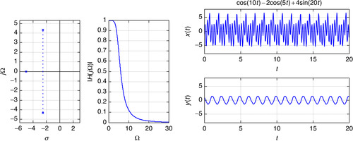
Consider the low-pass filtering of an analog signal x(t) = [−2cos(5t) + cos(10t) + 4sin(20t)]u(t) with MATLAB. The filter is a third-order low-pass Butterworth filter with a half-power frequency Ωhp = 5 rad/sec—that is, we wish to attenuate the frequency components of the frequencies 10 and 20 rad/sec. Design the desired filter and show how to do the filtering.
The design of the filter is done using the MATLAB function butter where besides the specification of the desired order, N = 3, and half-power frequency, Ωhp = 5 rad/sec, we also need to indicate that the filter is analog by including an 's' as one of the arguments. Once the coefficients of the filter are obtained, we could then either solve the differential equation from these coefficients or use the Fourier transform, which we choose to do. Symbolic MATLAB is thus used to compute the Fourier transform of the input X(Ω), and after generating the frequency response function H(jΩ) from the filter coefficients, we multiply these two to get Y(Ω), which is inversely transformed to obtain y(t). To obtain H(jΩ) symbolically we multiply the coefficients of the numerator and denominator obtained from butter by variables (jΩ)n where n corresponds to the order of the coefficient in the numerator or the denominator, and then add them. The poles of the designed filter and its magnitude response are shown in Figure 6.23, as well as the input x(t) and the output y(t). The following script was used for the filter design and the filtering of the given signal.
 |
| Figure 6.23 |
%%%%%%%%%%%%%%%%%%%
% Example 6.8 -- Filtering with Butterworth filter
%%%%%%%%%%%%%%%%%%%
clear all; clf
syms t w
x = cos(10 ∗ t) − 2 ∗ cos(5 ∗ t) + 4 ∗ sin(20 ∗ t); % input signal
X = fourier(x);
N = 3; Whp = 5;% filter parameters
[b, a] = butter(N, Whp, 's'), % filter design
W = 0:0.01:30; Hm = abs(freqs(b, a, W)); % magnitude response in W
% filter output
n = N:−1:0; U = (j ∗ w).^n
num = b − conj(U’); den = a − conj(U’);
Y = X ∗ H; % convolution property
y = ifourier(Y, t); % inverse Fourier
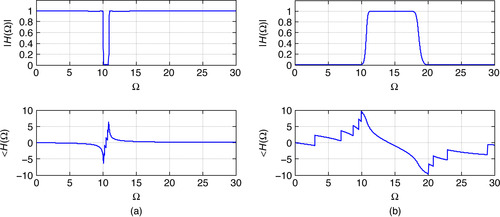
In this example we will compare the performance of Butterworth and Chebyshev low-pass filters in the filtering of an analog signal  using MATLAB. We would like the two filters to have the same half-power frequency.
The magnitude specifications for the low-pass Butterworth filter are
(6.54)
(6.55)
The Butterworth filter is designed by first determining the minimum order N and the half-power frequency Ωhp using the function buttord, and then finding the filter coefficients by means of the function butter. Likewise, for the design of the Chebyshev filter we use the function cheb1ord to find the minimum order and the cut-off frequency (the new Ωp is obtained from the halfpower frequency). The filtering is implemented using the Fourier transform as before.
There are two significant differences between the designed Butterworth and Chebyshev filters. Although both of them have the same half-power frequency, the transition band of the Chebyshev filter is narrower, [6.88 10], than that of the Butterworth filter, [5 10], indicating that the Chebyshev is a better filter. The narrower transition band is compensated by a lower minimum order of five for the Chebyshev compared to the six-order Butterworth. Figure 6.24 displays the poles of the Butterworth and the Chebyshev filters, their magnitude responses, as well as the input signal x(t) and the output y(t) for the two filters (the two perform very similarly).
 |
| Figure 6.24 |
%%%%%%%%%%%%%%%%%%%
% Example 6.9 -- Filtering with Butterworth and Chebyshev filters
%%%%%%%%%%%%%%%%%%%
clear all;clf
syms t w
x = cos(10 ∗ t) − 2 ∗ cos(5 ∗ t) + 4 ∗ sin(20 ∗ t); X = fourier(x);
wp = 5;ws = 10;alphamax = 0.1;alphamin = 15; % filter parameters
% butterworth filter
[N, whp] = buttord(wp, ws, alphamax, alphamin, 's')
[b, a] = butter(N, whp, 's')
% cheby1 filter
epsi = sqrt(10^(alphamax/10) − 1)
[N1, wn] = cheb1ord(wp, ws, alphamax, alphamin, 's'),
[b1, a1] = cheby1(N1, alphamax, wn, 's'),
% frequency responses
W = 0:0.01:30;
Hm = abs(freqs(b, a, W));
Hm1 = abs(freqs(b1, a1, W));
% generation of frequency response from coefficients
n = N:−1:0; n1 = N1:−1:0;
U = (j ∗ w).^n; U1 = (j ∗ w).^n1
num = b ∗ conj(U’); den = a ∗ conj(U’);
num1 = b1 ∗ conj(U1’); den1 = a1 ∗ conj(U1’)
H = num/den; % Butterworth LPF
H1 = num1/den1; % Chebyshev LPF
% output of filter
Y = X ∗ H;
Y1 = X ∗ H1;
y = ifourier(Y, t)
y1 = ifourier(Y1, t)
6.5.4. Frequency Transformations
As indicated before, the design of an analog filter is typically done by transforming the frequency of a normalized prototype low-pass filter. The frequency transformations were developed by Professor Ronald Foster [72] using the properties of reactance functions. The frequency transformations for the basic filters are given by:
(6.56)

Remarks
■ The low-pass to low-pass (LP-LP) and low-pass to high-pass (LP-HP) transformations are linear in the numerator and denominator; thus the number of poles and zeros of the prototype low-pass filter is preserved. On the other hand, the low-pass to band-pass (LP-BP) and low-pass to band-eliminating (LP-BE) transformations are quadratic in either the numerator or the denominator, so that the number of poles/zeros is doubled. Thus, to obtain a 2N th-order band-pass or band-eliminating filter the prototype low-pass filter should be of order N. This is an important observation useful in the design of these filters with MATLAB.
■ It is important to realize that only frequencies are transformed, and the magnitude of the prototype filter is preserved. Frequency transformations will be useful also in the design of discrete filters, where these transformations are obtained in a completely different way, as no reactance functions would be available in that domain.
To illustrate how the above transformations can be used to convert a prototype low-pass filter we use the following script. First a low-pass prototype filter is designed using butter, and then to this filter we apply the lowpass to highpass transformation with Ω0 = 40 (rad/sec) to obtain a high-pass filter. Let then Ω0= 6.32 (rad/sec) and BW = 10 (rad/sec) to obtain a band-pass and a band-eliminating filters using the appropriate transformations. The following is the script used. The magnitude responses are plotted with ezplot. Figure 6.25 shows the results.
 |
| Figure 6.25 |
clear all; clf
syms w
N = 5; [b, a] = butter(N, 1, 's') % low-pass prototype
omega0 = 40;BW = 10; omega1=sqrt(omega0); % transformation parameters
% low-pass prototype
n = N:−1:0;
U = (j ∗ w).^n; num = b ∗ conj(U’); den = a ∗ conj(U’);
H = num/den;
% low-pass to high-pass
num1 = b ∗ conj(U1’); den1 = a ∗ conj(U1’);
H1 = num1/den1;
% low-pass to band-pass
U2 = ((−w^2 + omega1^2)/(BW ∗ j ∗ w)).^n
num2 = b ∗ conj(U2’); den2 = a ∗ conj(U2’);
H2 = num2/den2;
% low-pass to band-eliminating
U3 = ((BW ∗ j ∗ w)/(−w^2 + omega1^2)).^n
num3 = b ∗ conj(U3’); den3 = a ∗ conj(U3’);
H3 = num3/den3
6.5.5. Filter Design with MATLAB
The design of filters, analog and discrete, is simplified by the functions that MATLAB provides. Functions to find the filter parameters from magnitude specifications, as well as functions to find the filter poles/zeros and to plot the designed filter magnitude and phase responses, are available.
Low-Pass Filter Design
The design procedure is similar for all of the approximation methods (Butterworth, Chebyshev, elliptic) and consists of both
■ Finding the filter parameters from loss specifications.
■ Obtaining the filter coefficients from these parameters.
Thus, to design an analog low-pass filter using the Butterworth approximation, the loss specifications αmax and αmin, and the frequency specifications, Ωp and Ωs are first used by the function buttord to determine the minimum order N and the half-power frequency Ωhp of the filter that satisfies the specifications. Then the function butter uses these two values to determine the coefficients of the numerator and the denominator of the designed filter. We can then use the function freqs to plot the designed filter magnitude and phase. Similarly, this applies for the design of low-pass filters using the Chebyshev or the elliptic design methods. To include the design of low-pass filters using the Butterworth, Chebyshev (two versions), and the elliptic methods we wrote the function analogfil.
function [b, a] = analogfil(Wp, Ws, alphamax, alphamin, Wmax, ind)
%%
%Analog filter design
%Parameters
%Input: loss specifications (alphamax, alphamin), corresponding
%frequencies (Wp,Ws), frequency range [0,Wmax] and indicator ind (1 for
%Butterworth, 2 for Chebyshev1, 3 for Chebyshev2 and 4 for elliptic).
%Output: coefficients of designed filter.
%Function plots magnitude, phase responses, poles and zeros of filter, and
%loss specifications
%%%
if ind == 1,% Butterworth low-pass
[N, Wn] = buttord(Wp, Ws, alphamax, alphamin, 's')
[b, a] = butter(N, Wn, 's')
elseif ind == 2, % Chebyshev low-pass
[N, Wn] = cheb1ord(Wp, Ws, alphamax, alphamin, 's')
[b, a] = cheby1(N, alphamax, Wn, 's')
elseif ind == 3, % Chebyshev2 low-pass
[N, Wn] = cheb2ord(Wp, Ws, alphamax, alphamin, 's')
[b, a] = cheby2(N, alphamin, Wn, 's')
else % Elliptic low-pass
[N, Wn] = ellipord(Wp, Ws, alphamax, alphamin, 's')
[b, a] = ellip(N, alphamax, alphamin, Wn, 's')
end
H = freqs(b, a, W); Hm = abs(H); Ha = unwrap(angle(H)) % magnitude (Hm) and phase (Ha)
N = length(W); alpha1 = alphamax ∗ ones(1, N); alpha2 = alphamin ∗ ones(1, N); % loss specs
subplot(221)
plot(W, Hm); grid; axis([0 Wmax 0 1.1 ∗ max(Hm)])
subplot(222)
plot(W, Ha); grid; axis([0 Wmax 1.1 ∗ min(Ha) 1.1 ∗ max(Ha)])
subplot(223)
splane(b, a)
subplot(224)
plot(W, −20 ∗ log10(abs(H))); hold on
plot(W, alpha1, 'r', W, alpha2, 'r'), grid; axis([0 max(W) −0.1 100])
hold off
To illustrate the use of analogfil consider the design of low-pass filters using the Chebyshev2 and the Elliptic design methods. The specifications for the designs are
 |
| Figure 6.26 |
% Example 6.11 -- Filter design using analogfil
%%%%%%%%%%%%%%%%%%%
clear all; clf
alphamax = 0.1;
alphamin = 60;
Wp =10; Ws = 15;
Wmax = 25;
ind = 4 % elliptic design
% ind = 3 % chebyshev2 design
[b, a] = analogfil(Wp, Ws, alphamax, alphamin, Wmax, ind)
The elliptic design is illustrated above. To obtain the Chebyshev2 design get rid of the comment symbol % in front of the corresponding indicator and put it in front of the one for the elliptic design.
General comments on the design of low-pass filters using Butterworth, Chebyshev (1 and 2), and Elliptic methods are:
■ The Butterworth and the Chebyshev2 designs are flat in the passband, while the others display ripples in that band.
■ For identical specifications, the obtained order of the Butterworth filter is much greater than the order of the other filters.
■ The phase of all of these filters is approximately linear in the passband, but not outside it. Because of the rational transfer functions for these filters, it is not possible to have linear phase over all frequencies. However, the phase response is less significant in the stopband where the magnitude response is very small.
■ The filter design functions provided by MATLAB can be used for analog or discrete filters. When designing an analog filter there is no constrain in the values of the frequency specifications and an 's' indicates that the filter being designed is analog.
General Filter Design
The filter design programs butter, cheby1, cheby2, and ellip allow the design of other filters besides low-pass filters. Conceptually, a prototype low-pass filter is designed and then transformed into the desired filter by means of the frequency transformations given before. The filter is specified by the order and cut-off frequencies. In the case of low-pass and high-pass filters the specified cut-off frequencies are scalar, while for band-pass and stopband filters the specified cut-off frequencies are given as a vector. Also recall that the frequency transformations double the order of the low-pass prototype for the band-pass and band-eliminating filters, so when designing these filters half of the desired order should be given.
To illustrate the general design consider:
(a) Using the cheby2 method, design a band-pass filter with the following specifications:
(b) Using the ellip method, design a band-stop filter with unit gain in the passbands and the following specifications:
■ order N = 20
■ α(Ω) = 0.1 dB in the passband
■ α(Ω) = 40 dB in the stopband
■ passband frequencies [10, 11] rad/sec
The following script is used.
%%%%%%%%%%%%%%%%%%%%%%%%%%%%
% Example 6.12 --- general filter design
%%%%%%%%%%%%%%%%%%%%%%%%%%%%
clear all;clf
N = 10;
[b, a] = ellip(N/2, 0.1, 40, [10 11], 'stop', 's') % elliptic band-stop
%[b, a] = cheby2(N, 60, [10 20], 's') % cheby2 bandpass
W = 0:0.01:30;
H = freqs(b, a, W);
Notice that the order given to ellip is 5 and 10 to cheby2 since a quadratic transformation will be used to obtain the notch and the band-pass filters from a prototype low-pass filter. The magnitude and phase responses of the two designed filters are shown in Figure 6.27.
6.6. What have we accomplished? What is next?
In this chapter we have illustrated the application of the Laplace and the Fourier analysis to the theories of control, communications, and filtering. As you can see, the Laplace transform is very appropriate for control problems where transients as well as steady-state responses are of interest. On the other hand, in communications and filtering there is more interest in steady-state responses and frequency characterizations, which are more appropriately treated using the Fourier transform. It is important to realize that stability can only be characterized in the Laplace domain, and that it is necessary when considering steady-state responses. The control examples show the importance of the transfer function and transient and steady-state computations. Block diagrams help to visualize the interconnection of the different systems. Different types of modulation systems are illustrated in the communication examples. Finally, this chapter provides an introduction to the design of analog filters. In all the examples, the application of MATLAB was illustrated.
Although the material in this chapter does not have sufficient depth, reserved for texts in control, communications, and filtering, it serves to connect the theory of continuous-time signals and systems with applications. In the next part of the book, we will consider how to process signals using computers and how to apply the resulting theory again in control, communications, and signal processing problems.
Cascade Implementation and Loading
 Carefully draw your circuit.
The transfer function of a filter H(s) = 1/(s + 1)2 is to be implemented by cascading two first-order filters Hi(s) = 1/(s + 1), i = 1, 2.
(a) Implement Hi(s) as a series RC circuit with input vi(t) and output vi + 1(t), i = 1, 2. Cascade two of these circuits and find the overall transfer function V3(s)/V1(s). Carefully draw the circuit.
(b) Use a voltage follower to connect the two circuits when cascaded and find the overall transfer function V3(s)/V1(s). Carefully draw the circuit.
(c) Use the voltage follower circuit to implement a new transfer function
Cascading LTI and LTV Systems
 where m(t) is a desired voice signal with bandwidth BW = 5 KHz that modulates the carrier cos(40,000πt) and q(t) is the rest of the signals available at the receiver. The low-pass filter is ideal with magnitude 1 and bandwidth BW. Assume the band-pass filter is also ideal and that the demodulator is cos(Ωct).
The receiver of an AM system consists of a band-pass filter, a demodulator, and a low-pass filter. The received signal is
(a) What is the value of Ωc in the demodulator?
(b) Suppose we input the received signal into the band-pass filter cascaded with the demodulator and the low-pass filter. Determine the magnitude response of the band-pass filter that allows us to recover m(t). Draw the overall system and indicate which of the components are LTI and which are LTV.
(c) By mistake we input the received signal into the demodulator, and the resulting signal into the cascade of the band-pass and the low-pass filters. If you use the band-pass filter obtained above, determine the recovered signal (i.e., the output of the low-pass filter). Would you get the same result regardless of what m(t) is? Explain.
Op-amps as Feedback Systems
An ideal operational amplifier circuit can be shown to be equivalent to a negative-feedback system. Consider the amplifier circuit in Figure 6.28 and its two-port network equivalent circuit to obtain a feedback system with input Vi(s) and output V0(s). What is the effect of A → ∞ on the above circuit?
 |
| Figure 6.28 |
RC Circuit as Feedback System
Consider a series RC circuit with input a voltage source vi(t) and output the voltage across the capacitor vo(t).
(a) Draw a negative-feedback system for the circuit using an integrator, a constant multiplier, and an adder.
(b) Let the input be a battery (i.e., vi(t) = Au(t)). Find the steady-state error e(t) = vi(t) − vo(t).
RLC Circuit as Feedback System
A resistor R, a capacitor C, and an inductor L are connected in series with a source vi(t). Consider the output of the voltage across the capacitor vo(t). Let R = 1Ω, C = 1 F and L = 1 H.
(a) Use integrators and adders to implement the differential equation that relates the input vi(t) and the output vo(t) of the circuit.
(b) Obtain a negative-feedback system block diagram with input Vi(s) and output V0(s). Determine the feedforward transfer function G(s) and the feedback transfer function H(s) of the feedback system.
(c) Find an equation for the error E(s) = Vi(s) − V0(s)H(s) and determine its steady-state response when the input is a unit-step signal (i.e., Vi(s) = 1/s).
Ideal and Lossy Integrators
 where X(s) and Y(s) are the Laplace transforms of the input x(t) and the output y(t) of the feedback system. Sketch the magnitude response of this system and determine the type of filter it is.
An ideal integrator has a transfer function 1/s, while a lossy integrator has a transfer function 1/(s + K).
(a) Determine the feedforward transfer function G(s) and the feedback transfer function H(s) of a negative-feedback system that implements the overall transfer function
(b) If we let G(s) = s in the previous feedback system, determine the overall transfer function Y(s)/X(s) where X(s) and Y(s) are the Laplace transforms of the input x(t) and the output y(t) of this new feedback system. Sketch the magnitude response of the overall system and determine the type of filter it is.
Feedback Implementation of an All-Pass System
Suppose you would like to obtain a feedback implementation of an all-pass filter
(a) Determine if the T(s) is the transfer function corresponding to an all-pass filter by means of the poles and zeros of T(s).
(b) Determine the feedforward transfer function G(s) and the feedback transfer function H(s) of a negative-feedback system that has T(s) as its overall transfer function.
(c) Would it be possible to implement T(s) using a positive-feedback system? If so, indicate its feedforward transfer function G(s) and the feedback transfer function H(s).
Filter Stabilization
 which is unstable given that one of its poles is in the right-hand s-plane.
The transfer function of a designed filter is
(a) Consider stabilizing G(s) by means of negative feedback with a gain K > 0 in the feedback. Determine the range of values of K that would make the stabilization possible.
(b) Use the cascading of an all-pass filter Ha(s) with the given G(s) to stabilize it. Give Ha(s). Would it be possible for the resulting filter to have the same magnitude response as G(s)?
Error and Feedforward Transfer Function
 where H(s) = G(s)/(1 + G(s)) is the overall transfer function of the feedback system, find an expression for the error in terms of X(s), N(s), and D(s). Use this equation to determine the conditions under which the steady-state error is zero for x(t) = u(t).
Suppose the feedforward transfer function of a negative-feedback system is G(s) = N(s)/D(s), and the feedback transfer function is unity.
(a) Given that the Laplace transform of the error is
(b) If the input is x(t) = u(t), the denominator D(s) = (s + 1)(s + 2), and the numerator N(s) = 1, find an expression for E(s) and from it determine the initial value e(0) and the final value  of the error.
Product of Polynomials in s—MATLAB
 where Y(s) and X(s) are the Laplace transforms of the output y(t) and of the input x(t) of an LTI system, and N(s) and D(s) are polynomials in s, to find the output
 we need to multiply polynomials to get Y(s) before we perform partial fraction expansion to get y(t).
Given a transfer function
(a) Find out about the MATLAB function conv and how it relates to the multiplication of polynomials. Let P(s) = 1 + s + s2 and Q(s) = 2 + 3s + s2 + s3. Obtain analytically the product Z(s) = P(s)Q(s) and then use conv to compute the coefficients of Z(s).
(b) Suppose that X(s) = 1/s2, and we have N(s) = s + 1, D(s) = (s + 1)((s + 4)2 + 9). Use conv to find the numerator and the denominator polynomials of Y(s) = N1(s)/D1(s). Use MATLAB to find y(t), and to plot it.
(c) Create a function that takes as input the values of the coefficients of the numerators and denominators of X(s) and of the transfer function H(s) of the system and provides the response of the system. Show your function, and demonstrate its use with the X(s) and H(s) given above.
Feedback Error—MATLAB
 The Laplace transform of the error signal is E(s) = X(s) − Y(s)H(s),
Control systems attempt to follow the reference signal at the input, but in many cases they cannot follow particular types of inputs. Let the system we are trying to control have a transfer function G(s), and the feedback transfer function be H(s). If X(s) is the Laplace transform of the reference input signal, and Y(s) the Laplace transform of the output, then the close-loop transfer function is
(a) Find an expression for E(s) in terms of X(s), G(s), and H(s).
(b) Let x(t) = u(t) and the Laplace transform of the corresponding error be E1(s). Use the final value property of the Laplace transform to obtain the steady-state error e1ss.
(c) Let x(t) = tu(t) (i.e., a ramp signal) and E2(s) be the Laplace transform of the corresponding error signal. Use the final value property of the Laplace transform to obtain the steady-state error e2ss. Is this error value larger than the one above? Which of the two inputs u(t) and r(t) is easier to follow?
(d) Use MATLAB to find the partial fraction expansions of E1(s) and E2(s) and use them to find e1(t) and e2(t) and then plot them.
Wireless Transmission—MATLAB
 where 0 ≤ αi ≤ 1 are attenuations, Li are the distances from the transmitter to the receiver that the signal travels in the ith path i = 1, 2, c = 3 × 10⁸ m/sec, and the frequency shift ν is caused by the Doppler effect.
 where ν = 50η Hz, L0 = 1,000η, L1 = 10,000η, α0 = 1 − η, α1 = α0/10, and η is a random number between 0 and 1 with equal probability of being any of these values (this can be realized by using the rand MATLAB function). Generate the received signal for 10 different events, use Fs = 10,000 Hz as the sampling rate, and plot them together to observe the effects of the multipath and Doppler.
Consider the transmission of a sinusoid x(t) = cos(2πf0t) through a channel affected by multipath and Doppler. Let there be two paths, and assume the sinusoid is being sent from a moving transmitter so that a Doppler frequency shift occurs. Let the received signal be
(a) Let f0 = 2 KHz, ν = 50 Hz, α0 = 1, α1 = 0.9, and L0 = 10,000 meters. What would be L1 if the two sinusoids have a phase difference of π/2?
(b) Is the received signal r(t), with the parameters given above but L1 = 10,000, periodic? If so, what would be its period and how much does it differ from the period of the original sinusoid? If x(t) is the input and r(t) the output of the transmission channel, considered a system, is it linear and time invariant? Explain.
(c) Sample the signals x(t) and r(t) using a sampling frequency Fs = 10 KHz. Plot the sampled sent x(nTs) and received r(nTs) signals for n = 0 to 2000.
(d) Consider the situation where f0 = 2 KHz, but the parameters of the paths are random, trying to simulate real situations where these parameters are unpredictable, although somewhat related. Let
RLC Implementation of Low-Pass Butterworth Filters
 That is, it is a second-order Butterworth filter.
Consider the RLC circuit shown in Figure 6.29 where R = 1 Ω.
 |
| Figure 6.29 |
(a) Determine the values of the inductor and the capacitor so that the transfer function of the circuit when the output is the voltage across the capacitor is
(b) Find the transfer function of the circuit, with the values obtained in (a) for the capacitor and the inductor, when the output is the voltage across the resistor. Carefully sketch the corresponding frequency response and determine the type of filter it is.
Design of Low-Pass Butterworth/Chebyshev Filters
The specifications for a low-pass filter are:
■ Ωp = 1500 rad/sec, αmax = 0.5 dBs
■ Ωs = 3500 rad/sec, αmin = 30 dBs
(a) Determine the minimum order of the low-pass Butteworth filter and compare it to the minimum order of the Chebyshev filter that satisfy the specifications. Which is the smaller of the two?
(b) Determine the half-power frequencies of the designed Butterworth and Chebyshev low-pass filters by letting α(Ωp) = αmax. Use the minimum orders obtained above.
(c) For the Butterworth and the Chebyshev designed filters, find the loss function values at Ωp and Ωs. How are these values related to the αmax and αmin specifications? Explain.
(d) If new specifications for the passband and stopband frequencies are Ωp = 750 rad/sec and Ωs = 1750 rad/sec, respectively, are the minimum orders of the Butterworth and the Chebyshev filters changed? Explain.
Low-Pass Butterworth Filters
The loss at a frequency Ω = 2000 rad/sec is α(2000) = 19.4 dBs for a fifth-order low-pass Butterworth filter. If we let α(Ωp) = αmax = 0.35 dBs, determine
Design of Low-Pass Butterworth/Chebyshev Filters
The specifications for a low-pass filter are:
■ α(0) = 20 dBs
■ Ωp = 1500 rad/sec, α1 = 20.5 dBs
■ Ωs = 3500 rad/sec, α2 = 50 dBs
(a) Determine the minimum order of the low-pass Butterworth and Chebyshev filters, and determine which is smaller.
(b) Give the transfer function of the designed low-pass Butterworth and Chebyshev filters (make sure the dc loss is as specified).
(c) Determine the half-power frequency of the designed filters by letting α(Ωp) = αmax.
(d) Find the loss function values provided by the designed filters at Ωp and Ωs. How are these values related to the αmax and αmin specifications? Explain. Which of the two filters provides more attenuation in the stopband?
(e) If new specifications for the passband and stopband frequencies are Ωp = 750 rad/sec and Ωs = 1750 rad/sec, respectively, are the minimum orders of the filter changed? Explain.
Butterworth, Chebyshev, and Elliptic Filters—MATLAB
Design an analog low-pass filter satisfying the following magnitude specifications:
■ αmax = 0.5 dB; αmin = 20 dB
■ Ωp = 1000 rad/sec; Ωs = 2000 rad/sec
(a) Use the Butterworth method. Plot the poles and zeros and the magnitude and phase of the designed filter. Verify that the specifications are satisfied by plotting the loss function.
(b) Use the Chebyshev method cheby1. Plot the poles and zeros and the magnitude and phase of the designed filter. Verify that the specifications are satisfied by plotting the loss function.
(c) Use the elliptic method. Plot the poles and zeros and the magnitude and phase of the designed filter. Verify that the specifications are satisfied by plotting the loss function.
(d) Compare the three filters and comment on their differences.
Chebyshev Filter Design—MATLAB
Consider the following low-pass filter specifications:
■ αmax = 0.1 dB; αmin = 60 dB
■ Ωp = 1000 rad/sec; Ωs = 2000 rad/sec
(a) Use MATLAB to design a Chebyshev low-pass filter that satisfies the above specifications. Plot the poles and zeros and the magnitude and phase of the designed filter. Verify that the specifications are satisfied by plotting the loss function.
(b) Compute the half-power frequency of the designed filter.
Getting Rid of 60-Hz Hum with Different Filters—MATLAB
 is recorded as y(t) = x(t) + cos(120πt)—that is, as the desired signal but with a 60-Hz hum. We would like to get rid of the hum and recover the desired signal. Use symbolic MATLAB to plot x(t) and y(t).
A desirable signal
Consider the following three different alternatives (use symbolic MATLAB to implement the filtering and use any method to design the filters):
(a) Design a band-eliminating filter to get rid of the 60-Hz hum in the signal. Plot the output of the band-eliminating filter.
(b) Design a high-pass filter to get the hum signal and then subtract it from y(t). Plot the output of the high-pass filter.
(d) Is any of these alternatives better than the others? Explain.
Demodulation of AM—MATLAB
 where the messages mi(t), i = 1, 2 are the outputs of a low-pass Butterworth filter with inputs
 respectively. Suppose we are interested in recovering the message m1(t).
The signal at the input of an AM receiver is
(a) Design a 10th-order low-pass Butterworth filter with half-power 10 rad/sec. Implement this filter using MATLAB and find the two messages mi(t), i = 1, 2 using the indicated inputs xi(t), i = 1, 2, and plot them.
(b) To recover the desired message m1(t), first use a band-pass filter to obtain the desired signal containing m1(t) and to suppress the other. Design a band-pass Butterworth filter with a bandwidth of 10 rad/sec, centered at 20 rad/sec and order 10 that will pass the signal m1(t) cos(20t) and reject the other signal.
(c) Multiply the output of the band-pass filter by a sinusoid cos(20t) (exactly the carrier in the transmitter), and low-pass filter the output of the mixer (the system that multiplies by the carrier frequency cosine). Design a low-pass Butterworth filter of bandwidth 10 rad/sec, and order 10 to filter the output of the mixer.
(d) Use MATLAB to display the different spectra. Compute and plot the spectrum of m1(t), u(t), the output of the band-pass filter, the output of the mixer, and the output of the low-pass filter. Write numeric functions to compute the analog Fourier transform and its inverse.
Quadrature AM—MATLAB
 Suppose that at the receiver we receive s(t) and that we only need to demodulate it to obtain mi(t), i = 1, 2. Design a low-pass Butterworth filter of order 10 and a half-power frequency 10 rad/sec (the bandwidth of the messages).
Suppose we would like to send the two messages mi(t), i = 1, 2, created in Problem 6.20 using the same bandwidth and to recover them separately. To implement this, consider the QAM approach where the transmitted signal is
(a) Use MATLAB to plot s(t) and its magnitude spectrum |S(Ω)|. Write numeric functions to compute the analog Fourier transform and its inverse.
(b) Multiply s(t) by cos(50t), and filter the result using the low-pass filter designed before. Use MATLAB to plot the result and to find and plot its magnitude spectrum.
(c) Multiply s(t) by sin(50t), and filter the result using the low-pass filter designed before. Use MATLAB to plot the result and to find and plot its magnitude spectrum.
(d) Comment on your results.
..................Content has been hidden....................
You can't read the all page of ebook, please click here login for view all page.