
Chapter 5. Frequency Analysis
The Fourier Transform
Imagination is the beginning of creation. You imagine what you desire, you will what you imagine, and at last you create what you will.
George Bernard Shaw (1856–1950) Irish dramatist
5.1. Introduction
In this chapter we continue the frequency analysis of signals. In particular, we will concentrate in the following issues:
■ Generalization of the Fourier series—The frequency representation of signals as well as the frequency response of systems are tools of great significance in signal processing, communications, and control theory. In this chapter we will complete the Fourier representation of signals by extending it to aperiodic signals. By a limiting process the harmonic representation of periodic signals is extended to the Fourier transform, a frequency-dense representation for nonperiodic signals. The concept of spectrum introduced for periodic signals is generalized for both finite-power and finite-energy signals. Thus, the Fourier transform measures the frequency content of a signal, and unifies the representation of periodic and aperiodic signals.
■ Laplace and Fourier transform—In this chapter the connection between the Laplace and the Fourier transforms will be highlighted for computational and analytical reasons. The Fourier transform turns out to be a very important case of the Laplace transform for signals of which the region of convergence includes the jΩ axis. There are, however, signals where the Fourier transform cannot be obtained from the Laplace transform; for those cases, properties of the Fourier transform will be used. The duality of the direct and inverse transforms is of special interest in computing the Fourier transform.
■ Basics of filtering—Filtering is an important application of the Fourier transform. The Fourier representation of signals and the eigenfunction property of LTI systems provide the tools to change the frequency content of a signal by processing it with an LTI system with a desired frequency response.
■ Modulation and communications—The idea of changing the frequency content of a signal via modulation is basic in analog communications. Modulation allows us to send signals over the airwaves using antennas of reasonable sizes. Voice and music are relative low-frequency signals that cannot be easily radiated without the help of modulation. Continuous-wave modulation changes the amplitude, the frequency, or the phase of a sinusoidal carrier of frequency much greater than the frequencies present in the message we wish to transmit.
5.2. From the Fourier Series to the Fourier Transform
In practice there are no periodic signals—such signals would have infinite supports and exact periods, which are not possible. Since only finite-support signals can be processed numerically, signals in practice are treated as aperiodic. To obtain the Fourier representation of aperiodic signals, we use the Fourier series representation in a limiting process.
An aperiodic, or nonperiodic, signal x(t) can be thought of as a periodic signal  with an infinite period. Using the Fourier series representation of this signal and a limiting process we obtain a pair
(5.1)

(5.2)

Any aperiodic signal can be assumed to be periodic with an infinite period. That is, an aperiodic signal x(t) can be expressed as

Letting ΔΩ = 2π/T0 = Ω0 be the frequency interval between harmonics, we can then write the above equations as
The Fourier transform measures the frequency content of a signal. As we will see, time and frequency are complementary, thus the characterization in one domain provides information that is not clearly available in the other.
Remarks
■ Although we have obtained the Fourier transform from the Fourier series, the Fourier transform of a periodic signal cannot be obtained from the above integral. Consider x(t) = cos(Ω0t), −∞ < t < ∞, which is periodic of period 2π/Ω0. If you attempt to compute its Fourier transform using the integral you do not have a well-defined problem (try to obtain the integral to convince yourself). But it is known from the line spectrum that the power of this signal is concentrated at the frequencies ±Ω0, so somehow we should be able to find its Fourier transform. Sinusoids are basic functions.
■ On the other hand, if you consider a decaying exponential x(t) = e−|a|tsignal, which has finite energy and is absolutely integrable and has a Laplace transform that is valid on the jΩ axis (i.e., the region of convergence X(s) includes this axis), then its Fourier transform is simply the Laplace transform X(s) computed at s = jΩ, as we will see. There is no need for the integral formula in this case, although if you apply it your result coincides with the one from the Laplace transform.
■ Finally, consider finding the Fourier transform of a sinc function (which is the impulse response of a low-pass filter as we see later). Neither the integral nor the Laplace transform can be used to find it. For this signal, we need to exploit the duality that exists between the direct and the inverse Fourier transforms (Notice the duality in(5.1) and (5.2)).
5.3. Existence of the Fourier Transform
The Fourier transform
■ x(t) is absolutely integrable or the area under |x(t)| is finite.
■ x(t) has only a finite number of discontinuites as well as maxima and minima.
From the definitions of the direct and the inverse Fourier transforms—both being infinite integrals—one wonders whether they exist in general, and if so how to most efficiently compute them. Commenting on the existence conditions, Professor E. Craig [17] wrote:
It appears that almost nothing has a Fourier transform—nothing except practical communication signals. No signal amplitude goes to infinity and no signal lasts forever; therefore, no practical signal can have infinite area under it, and hence all have Fourier transforms.
5.4. Fourier Transforms from the Laplace Transform
The region of convergence of the Laplace transform X(s) indicates the region in the s-plane where X(s) is defined. The following applies to signals whether they are causal, anti-causal, or noncausal.
If the region of convergence (ROC) of  contains the jΩ axis, so that X(s) can be defined for s = jΩ, then
(5.3)

The following rules of thumb will help you get a better understanding of the time-frequency relationship of a signal and its Fourier transform, and the best way to compute it. On a first reading the use of these rules might not be obvious, but they will be helpful in understanding the discussions that follow and you might want to come back to these rules.
Rules of Thumb for Computing the Fourier Transform of a Signal x(t)
■ If x(t) has a finite time support and in that support x(t) is finite, its Fourier transform exists. To find it use the integral definition or the Laplace transform of x(t).
■ If x(t) has a Laplace transform X(s) with a region of convergence including the jΩ axis, its Fourier transform is X(s)|s = jΩ.
■ If x(t) is periodic of infinite energy but finite power, its Fourier transform is obtained from its Fourier series using delta functions.
■ If x(t) is none of the above, if it has discontinuities (e.g., x(t) = u(t)) or it has discontinuities and it is not finite energy (e.g., x(t) = cos(Ω0t)u(t)), or it has possible discontinuities in the frequency domain even though it has finite energy (e.g., x(t) = sinc(t)), use properties of the Fourier transform.
Keep in mind to
■ Consider the Laplace transform if the interest is in transients and steady state, and the Fourier transform if steady-state behavior is of interest.
■ Represent periodic signals by their Fourier series before considering their Fourier transforms.
■ Attempt other methods before performing integration to find the Fourier transform.
Discuss whether it is possible to obtain the Fourier transform of the following signals using their Laplace transforms:
(a) 
(b) 
(c) 
Solution
(a) The Laplace transform of x1(t) is X1(s) = 1/s with a region of convergence corresponding to the open right s-plane, or ROC = {s = σ + jΩ : σ > 0, −∞ < Ω < ∞}, which does not include the jΩ axis, so the Laplace transform cannot be used to find the Fourier transform of x1(t).
(b) The signal x2(t) has as Laplace transform X2(s) = 1/(s + 2) with a region of convergence ROC = {s = σ + jΩ : σ > −2, −∞ < Ω < ∞} containing the jΩ axis. Then the Fourier transform of x2(t) is
5.5. Linearity, Inverse Proportionality, and Duality
Many of the properties of the Fourier transform are very similar to those of the Fourier series or of the Laplace transform, which is to be expected given the strong connection among these transformations. The linearity and the duality between time and frequency of the Fourier transform will help us determine the transform of signals that do not satisfy the existence conditions given before.
5.5.1. Linearity
Just like the Laplace transform, the Fourier transform is linear.
If  and
and  , for constants α and β, we have that
(5.4)
Suppose you create a periodic sine
Solution
The Laplace transforms of v(t) and y(t) are

5.5.2. Inverse Proportionality of Time and Frequency
It is very important to realize that frequency is inversely proportional to time, and that as such, time and frequency signal characterizations are complementary. Consider the following examples to illustrate this.
■ The impulse signal x1(t) = δ(t), although not a regular signal, has finite support (its support is only at t = 0 as the signal is zero everywhere else). It is also absolutely integrable, so it has a Fourier transform

■ Consider then the opposite case: A signal that is constant for all times, that does not change, or a dc signal x2(t) = A, −∞ < t < ∞. We know that the frequency of Ω = 0 is assigned to it since the signal does not vary at all. The Fourier transform cannot be found by means of the integral because x2(t) is not absolutely integrable, but we can verify that it is given by X2(Ω) = 2πAδ(Ω) (we will formally show this using the duality property). In fact, the inverse Fourier transform is

■ To appreciate the transition from the dc signal to the impulse signal, consider a pulse signal x3(t) = A[u(t + τ/2) − u(t − τ/2)]. This signal has finite energy, and its Fourier transform can be found using its Laplace transform. We have
(5.5)

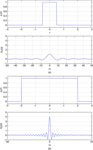
If we let A = 1/τ (so that the area of the pulse is unity), and let τ → 0, the pulse x3(t) becomes a delta function δ(t) in the limit and the sinc function expands (for τ → 0, X3(Ω) is not zero for any finite value) to become unity. On the other hand, if we let τ → ∞, the pulse becomes a constant signal A extending from −∞ to ∞, and the Fourier transform gets closer and closer to δ(Ω) (the sinc function becomes zero at values very close to zero and the amplitude at Ω = 0 becomes larger and larger, although the area under the curve remains constant). As shown above, X3(Ω) = 2πAδ(Ω) is the transform of x3(t) = A, −∞ < t < ∞.
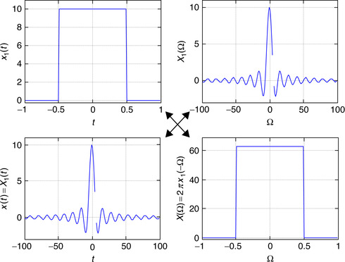
■ To illustrate the transition in the Fourier transform as the time support increases, we used the following MATLAB script to compute the Fourier transform of pulses of the same amplitude A = 1 but different time supports 1 and 4. The script below shows the case when the support is 1, but it can be easily changed to get the support of 4. The symbolic MATLAB function fourier computes the Fourier transform. The results are shown in Figure 5.1.
%%%%%%%%%%%%%%%%%%%%%
% Time-frequency relation
%%%%%%%%%%%%%%%%%%%%%
syms t w
x = heaviside(t + 0.5) − heaviside(t − 0.5);
subplot(211)
ezplot(x, [− 3]);axis([−3 3 − 0.1 1.1]);grid
X = fourier(x) % Fourier transform
subplot(212)
ezplot(X, [−50 50]); axis([−50 50 −1 5]);grid
In summary, the support of X(Ω) is inversely proportional to the support of x(t). If x(t) has a Fourier transform X(Ω) and α ≠ 0 is a real number, then x(αt) is an
■ Contracted (α > 1),
■ Contracted and reflected (α < −1),
■ Expanded (0 < α < 1),
■ Expanded and reflected (−1 < α < 0), or
■ Simply reflected (α = −1)
(5.6)
First let us mention that the symbol ⇔ means that to a signal x(t) in the time domain (on the left) there corresponds a Fourier transform X(Ω) in the frequency domain (on the right). This is not an equality—far from it!
Consider a pulse x(t) = u(t) − u(t − 1). Find the Fourier transform of x1(t) = x(2t).
Solution
The Laplace transform of x(t) is

 |
| Figure 5.2 |

Apply the reflection property to find the Fourier transform of x(t) = e−a|t|, a > 0. For a = 1, plot using MATLAB the signal and its magnitude and phase spectra.
Solution
The signal x(t) can be expressed as x(t) = e−atu(t) + eatu(−t) = x1(t) + x1(−t). The Fourier transform of x1(t) is
If a = 1, using MATLAB the signal x(t) = e−|t| and its magnitude and phase spectra are computed and plotted as shown in Figure 5.3. Since X(Ω) is real and positive, the corresponding phase spectrum is zero. This signal is called low-pass since its energy is concentrated in the low frequencies.

5.5.3. Duality
Besides the inverse relationship of frequency and time, by interchanging the frequency and the time variables in the definitions of the direct and the inverse Fourier transform (see (5.1) and (5.2)) similar equations are obtained. Thus, the direct and the inverse Fourier transforms are dual.
To the Fourier transform pair
(5.7)
(5.8)

Remarks
■ This duality property allows us to obtain the Fourier transform of signals for which we already have a Fourier pair and that would be difficult to obtain directly. It is thus one more method to obtain the Fourier transform, besides the Laplace transform and the integral definition of the Fourier transform.
■ When computing the Fourier transform of a constant signal, x(t) = A, we indicated that it would be X(Ω) = 2πAδ(Ω). Indeed, we have the dual pairs
(5.9)
Use the duality property to find the Fourier transform of the sinc signal
Solution
The Fourier transform of the sinc signal cannot be found using the Laplace transform or the integral definition of the Fourier transform. The duality property provides a way to obtain it. We found before, for τ = 1, the following pair of Fourier transforms:
Find the Fourier transform of x(t) = A cos(Ω0t) using duality.
Solution
The Fourier transform of x(t) cannot be computed using the integral definition since this signal is not absolutely integrable, or using the Laplace transform since x(t) does not have a Laplace transform. As a periodic signal, x(t) has a Fourier series representation and we will use it later to find its Fourier transform. For now, let us consider the Fourier pair
(5.10)
5.6. Spectral Representation
In this section, we consider first how to find the Fourier transform of periodic signals using the modulation property, and then consider Parseval's result for finite-energy signals. With these results, we will unify the spectral representation of both periodic and aperiodic signals.
5.6.1. Signal Modulation
One of the most significant properties of the Fourier transform is modulation. Its application to signal transmission is fundamental in communications.
■ Frequency shift: If X(Ω) is the Fourier transform of x(t), then we have the pair
(5.11)
■ Modulation: The Fourier transform of the modulated signal
(5.12)
(5.13)
The frequency shifting property is easily shown:

Remarks
■ As indicated before, amplitude modulation consists in multiplying an incoming signal x(t), or message, by a sinusoid of frequency higher than the maximum frequency of the incoming signal. The modulated signal is
■ Modulation using a sine, instead of a cosine, changes the phase of the Fourier transform of the incoming signal besides performing the frequency shift. Indeed,
■ According to the eigenfunction property of LTI systems, modulation systems are not LTI. Modulation shifts the frequencies at the input to new frequencies at the output. Nonlinear or time-varying systems are typically used as amplitude modulation transmitters.
Consider modulating a carrier cos(10t) with the following signals:
■ x1(t) = e−|t|, −∞ < t < ∞. Use MATLAB to find the Fourier transform of y1(t) = x1(t) cos(10t) and plot y1(t) and its magnitude and phase spectra.
■ x2(t) = 0.2[r(t + 5) − 2r(t) + r(t + 5)], where r(t) is the ramp signal. Use MATLAB to plot x2(t) and y2(t) = x2(t) cos(10t) and compute and plot the magnitude of their Fourier transforms.
Solution
• y1(t) = x1(t) cos(10t) = e−|t| cos(10t)−∞ < t < ∞
• y2(t) = x2(t) cos(10t) = 0.2[r(t + 5) − 2r(t) + r(t + 5)] cos(10t)
The signal x1(t) is very smooth, although of infinite support, and thus most of its frequency components are of low frequency. The signal x2(t) is not as smooth and has a finite support, so that its frequency components are mostly low pass but its spectrum also displays higher frequencies.
The MATLAB scripts used to compute the Fourier transform of the modulated signals and to plot the signals, their modulated versions, and the magnitude and phase of the Fourier transforms are very similar. The following script indicates how to generate y1(t) and how to find the magnitude and phase of its Fourier transform Y1(Ω). Notice the way the phase is computed.
%%%%%%%%%%%%%%%%%%%%%
% Example 5.7---Modulation
%%%%%%%%%%%%%%%%%%%%%
y1 = exp(−abs(t)). ∗ cos(10 ∗ t);
% magnitude and phase of Y1(Omega)
Y1 = fourier(y1); Ym = abs(Y1); Ya = atan(imag(Y1)/real(Y1));
The signal x2(t) is a triangular signal. The following script shows how to generate the signal x2(t). Instead of multiplying x2(t) by the cosine, we multiply it by the cosine-equivalent representation in complex exponentials, which will give better plots of the Fourier transforms when using ezplot.
m = heaviside(t + 5) − heaviside(t);
m1 = heaviside(t) − heaviside(t−5);
x2 = (t + 5) ∗ m + m1 ∗ (−t + 5); x2 = x2/5;
x = x2 ∗ exp(−j ∗ 10 ∗ t)/2; y = x2 ∗ exp(+j ∗ 10 ∗ t)/2;
X = fourier(x); Y = fourier(y);
Y2m = abs(X) + abs(Y); % magnitude of Y_2(Omega)
X2 = fourier(x2); X2m = abs(X2); % magnitude of X_2(Omega)
The results are shown in Figure 5.5.

Why Modulation?
The use of modulation to change the frequency content of a message from its baseband frequencies to higher frequencies makes its transmission over the airwaves possible. Let us explore why it is necessary to use modulation to transmit a music or a speech signal. Typically, acoustic signals such as music are audible up to frequencies of about 22 KHz, while speech signals typically display frequencies from about 100 Hz to about 5 KHz. Thus, music and speech signals are relatively low-frequency signals. When radiating a signal with an antenna, the length of the antenna is about a quarter of the wavelength,

5.6.2. Fourier Transform of Periodic Signals
By applying the frequency-shifting property to compute the Fourier transform of periodic signals, we are able to unify the Fourier representation of aperiodic as well as periodic signals.
For a periodic signal x(t) of period T0, we have the Fourier pair
(5.14)
Since a periodic signal x(t) is not absolutely integrable, its Fourier transform cannot be computed using the integral formula. But we can use its Fourier series
Remarks
■ When plotting |X(Ω)| versus Ω, which we call the Fourier magnitude spectrum, for a periodic signal x(t), we notice it is analogous to its line spectrum discussed before. Both indicate that the signal power is concentrated in multiples of the fundamental frequency, the only difference being in how the information is provided at each of the frequencies. The line spectrum displays the Fourier series coefficients at their corresponding frequencies, while the spectrum from the Fourier transform displays the concentration of the power at the harmonic frequencies by means of delta functions with amplitudes of 2π times the Fourier series coefficients. Thus, there is a clear relation between these two spectra, showing exactly the same information in slightly different form.
■ The Fourier transform of a cosine signal can now be computed directly as


Consider a periodic signal x(t) with a period
Solution
The given period x1(t) corresponds to a triangular signal. Its Laplace transform is


 |
| Figure 5.6 |
% Example 5.8---Fourier series
%%%%%%%%%%%%%%%%%%%%%
T0 = 1; N = 10; w0 = 2 ∗ pi/T0;
m = heaviside(t) − heaviside(t − T0/2);
m1 = heaviside(t − T0/2) − heaviside(t − T0);
x = t ∗ m + m1 ∗ (−t + T0); x = 2 * x; % periodic signal
[Xk, w] = fourierseries(x, T0, N); % Fourier coefficients, harmonic frequencies
% Fourier series approximation
for k = 1:N,
if k == 1;
x1 = abs(Xk(k));
else
x1 = x1 + 2 ∗ abs(Xk(k)) ∗ cos(w0 ∗ (k−1) ∗ t + angle(Xk(k)));
end
end
% sequence of Fourier coefficients and harmonic frequencies
k = 0:N−1; Xk1 = 2 ∗ pi ∗ Xk; wk = [−fliplr(k(2:N−1)) k] ∗ w0; Xk = [fliplr(Xk1(2:N − 1)) Xk1];
In this case, the Laplace transform simplifies the computation of the Xk values. Indeed, the Fourier series coefficients are given by
5.6.3. Parseval's Energy Conservation
We saw in Chapter 4 that for periodic signals having finite power but infinite energy, Parseval's theorem indicates how the power of the signal is distributed among the harmonic components. Likewise, for aperiodic signals of finite energy, an energy version of Parseval's result indicates how the signal energy is distributed over frequencies.
For a finite-energy signal x(t) with Fourier transform X(Ω), its energy is conserved when going from the time to the frequency domain, or
(5.15)

The plot |X(Ω)|2 versus Ω is called the energy spectrum of x(t), and it displays how the energy of the signal is distributed over frequency.
This energy conservation property is shown using the inverse Fourier transform. The finite-energy signal of x(t) can be computed in the frequency domain by

Parseval's result helps us to understand better the nature of an impulse δ(t). It is clear from its definition that the area under an impulse is unity, which means δ(t) is absolutely integrable, but does it have finite energy? Show how Parseval's result can help resolve this issue.
Solution
Let's consider this from the frequency point of view, using Parseval's result. The Fourier transform of δ(t) is unity for all values of frequency and as such its energy is infinite. Such a result seems puzzling, because δ(t) was defined as the limit of a pulse of finite duration and unity area. This is what happens if
Consider a pulse p(t) = u(t + 1) − u(t − 1). Use its Fourier transform P(Ω) and Parseval's result to show that


5.6.4. Symmetry of Spectral Representations
Now that the Fourier representation of aperiodic and periodic signals is unified, we can think of just one spectrum that accommodates both finite-energy as well as infinite-energy signals. The word spectrum is loosely used to mean different aspects of the frequency representation. In the following we provide definitions and the symmetry characteristic of the spectrum of real-valued signals.
If X(Ω) is the Fourier transform of a real-valued signal x(t), periodic or aperiodic, the magnitude |X(Ω)| is an even function of Ω:
(5.16)
(5.17)

To show this, consider the inverse Fourier transform of a real-valued signal x(t),

Remarks
■ Clearly, if the signal is complex, the above symmetry will not hold. For instance, if , using the frequency-shift property its Fourier transform is
■ It is important to recognize the meaning of “negative” frequencies. In reality, only positive frequencies exist and can be measured, but as shown the spectrum, magnitude or phase, of a real-valued signal requires negative frequencies. It is only under this context that negative frequencies should be understood as necessary to generate “real-valued” signals.
Use MATLAB to compute the Fourier transform of the following signals:
(a) 
(b) 
Solution
Three possible ways to compute the Fourier transforms of these signals using MATLAB are: (1) find their Laplace transforms as in Chapter 3 using laplace and compute the magnitude and phase function by letting s = jΩ, (2) by using the symbolic function fourier, and (3) sample x(t) and find its Fourier transform (this requires sampling theory—see Chapter 7).
The following script is used to compute and plot the signal x2(t) = e−tu(t) and the magnitude and phase of its Fourier transform using symbolic MATLAB. A similar script is used for x1(t).
%%%%%%%%%%%%%%%%%%%%%
% Example 5.11
%%%%%%%%%%%%%%%%%%%%%
symm t
x2 = exp(−t) ∗ heaviside(t);
X2 = fourier(x2)
X2m = sqrt((real(X2))^2 + (imag(X2))^2; % magnitude
X2p = imag(log(X2); % phase
Notice the way that the magnitude and the phase are computed. To compute the magnitude we use
The computation of the phase is complicated by the lack of the function atan2 in symbolic MATLAB, which extends the principal values of the inverse tangent to (−π, π] by considering the sign of the real part. The phase computation can be done by using the log function; indeed
Analytically, the phase of the Fourier transform of x1(t) = u(t) − u(t − 1) can be found by considering the advanced signal z(t) = x1(t + 0.5) = u(t + 0.5) − u(t − 0.5) with Fourier transform


It is not always the case that the Fourier transform is a complex-valued function. Consider the signals
(a) 
(b) 
Solution
(a) The Fourier transform of x(t) is

(b) The signal y(t) = 2x(t) cos(Ω0t) is a band-pass signal. It is not as smooth as the signals in the above example given that the concentration of
The bandwidth of a signal x(t) is the support—on the positive frequencies—of its Fourier transform X(Ω). There are different definitions of the bandwidth of a signal depending on how the support of its Fourier transform is measured. We will discuss some of the bandwidth measures used in filtering and in communications in Chapter 6.
The bandwidth together with the information about the signal being low-pass or band-pass provides a good characterization of the signal. The concept of the bandwidth of a filter that was discussed in circuit theory is one of its possible definitions; other possible definitions will be introduced in Chapter 6. The spectrum analyzer, a device used to measure the spectral characteristics of a signal, will be presented in section 5.7.4 after considering filtering.
5.7. Convolution and Filtering
The modulation and the convolution integral properties are the most important properties of the Fourier transform. Modulation is essential in communications, and the convolution property is basic in the analysis and design of filters.
If the input x(t) (periodic or aperiodic) to a stable LTI system has a Fourier transform X(Ω), and the system has a frequency response  where h(t) is the impulse response of the system, the output of the LTI system is the convolution integral y(t) = (x ∗ h)(t), with Fourier transform
(5.18)
(5.19)
This can be shown by considering the eigenfunction property of LTI systems. The Fourier representation of x(t), if aperiodic, is an infinite summation of complex exponentials ejΩt multiplied by complex constants X(Ω), or


If x(t) is periodic of period T0 (or fundamental frequency Ω0 = 2π/T0), then

An important consequence of the convolution property, just like in the Laplace transform, is that the ratio of the Fourier transforms of the input and the output gives the frequency response of the system, or
(5.20)
Remarks
■ It is important to keep in mind the following connection between the impulse response h(t), the transfer function H(s), and the frequency response H(jΩ) that characterize an LTI system:

■ As the Fourier transform of a real-valued function, the impulse response h(t), the function H(jΩ) has a magnitude |H(jΩ)| and a phase ∠H(jΩ), which are even and odd functions of the frequency Ω.
■ The convolution property relates to the processing of an input signal by an LTI system. But it is possible, in general, to consider the case of convolving two signals x(t) and y(t) to get z(t) = [x ∗ y](t), in which case we have that Z(Ω) = X(Ω)Y(Ω) where X(Ω) and Y(Ω) are the Fourier transforms of x(t) and y(t).
5.7.1. Basics of Filtering
The most important application of LTI systems is filtering. Filtering consists in getting rid of undesirable components of a signal. A typical example is when noise η(t) is added to a desired signal x(t) (i.e., y(t) = x(t) + η(t)), and the spectral characteristics of x(t) and the noise η(t) are known. The problem then is to design a filter, or an LTI system, that will get rid of the noise as much as possible. The filter design consists in finding a transfer function H(s) = B(s)/A(s) that satisfies certain specifications that will allow getting rid of the noise. Such specifications are typically given in the frequency domain. This is a rational approximation problem, as we look for the coefficients of the numerator and denominator of H(s) that make H(jΩ) in magnitude and phase approximate the filter specifications. The designed filter should be implementable and stable. In this section we discuss the basics of filtering and in Chapter 6 we introduce the filter design.
Frequency-discriminating filters keep the frequency components of a signal in a certain frequency band and attenuate the rest. Filtering an aperiodic signal x(t) represented by its Fourier transform X(Ω) with magnitude |X(Ω)| and phase ∠X(Ω), using a filter with frequency response H(jΩ), gives an output y(t) with a Fourier transform of
If the input signal x(t) is periodic of period T0, or fundamental frequency Ω0 = 2π/T0, the Fourier transform of the output is
(5.21)

The above shows that independent of whether the input signal x(t) is periodic or aperiodic, the output signal y(t) has the frequency components allowed through by the filter.
Consider how to obtain a dc source using a full-wave rectifier and a low-pass filter (it keeps only the low-frequency components). Let the full-wave rectified signal x(t) be the input of the filter and let the output of the filter be y(t). We want y(t) = 1 volt. The rectifier and the low-pass filter constitute a system that converts alternating into direct voltage.
Solution
We found in Chapter 4 that the Fourier series coefficients of x(t) = |cos(π t)|, − ∞ < t < ∞, are given by


Windowing is a time-domain process by which we select part of a signal. This is done by multiplying the signal by a “window” signal w(t). Consider the rectangular window
Solution
Windowing is the dual of filtering. In this case, the signal y(t) has the support determined by the window, or −Δ ≤ t ≤ Δ, and as such it is zero outside this interval. The window gets rid of parts of the signal outside its support. The signal y(t) can be written as


5.7.2. Ideal Filters
Frequency-discriminating filters that keep low-, middle-, and high-frequency components, or a combination of these, are called low-pass, band-pass, high-pass, and multiband filters, respectively. A band-eliminating or notch filter gets rid of middle-frequency components. It is also possible to have an all-pass filter that although it does not filter out any of the input frequency components, it changes the phase of the input signal.
The magnitude frequency response of an ideal low-pass filter is given by
An ideal band-pass filter has a magnitude response


From these definitions, we have that the ideal band-stop filter has as magnitude response of

Remarks
■ If hlp(t) is the impulse response of a low-pass filter, applying the modulation property we get that 2hlp(t) cos(Ω0t) (where Ω0 >> Ω1and Ω1is the cut-off frequency of the low-pass filter) corresponds to the impulse response of a band-pass filter centered around Ω0. Indeed, its Fourier transform is given by
■ A zero-phase ideal low-pass filter Hlp(jΩ) = u(Ω + Ω1) − u(Ω − Ω1) has as impulse response a sinc function with a support from −∞ to ∞. This ideal low-pass filter is clearly noncausal as its impulse response is not zero for negative values of time t. To make it causal we could approximate its impulse response by a function h1(t) = hlp(t)w(t) where w(t) = u(t + τ) − u(t − τ) is a rectangular window where the value of τ is chosen so that outside the window the values of the impulse response hlp(t) are very close to zero. Although the Fourier transform of h1(t) is a very good approximation of the desired frequency response, the frequency response of h1(t) displays ringing around the cut-off frequency Ω1because of the rectangular window. Finally, we delay h1(t) by τ to get a causal filter with linear phase. That is, h1(t − τ) has as its magnitude response |H1(jΩ)| ≈ |Hlp(jΩ)| and its phase response is ∠H1(jΩ) = −τΩ. Although the above procedure is a valid way to obtain approximate low-pass filters with linear phase, they are not guaranteed to be rational and would be difficult to implement. Thus, other methods are used to design filters.
■ Since ideal filters are not causal they cannot be used in real-time applications—that is when the input signal needs to be processed as it comes to the filter. Imposing causality on the filter restricts the frequency response of the filter in significant ways. According to the Paley-Wiener integral condition, a causaland stable filter with frequency response H(jΩ) should satisfy the condition
(5.22)
■ That ideal filters are not realizable can be understood also by considering what it means to make the magnitude response of a filter zero in some frequency bands. A measure of attenuation is given by the loss function in decibels, defined as

The Gibb's phenomenon, which we mentioned when discussing the Fourier series of periodic signals with discontinuities, consists in ringing around these discontinuities. To see this, consider a periodic train of square pulses x(t) of period T0 displaying discontinuities at kT0/2, for k = ±1, ±2, …. Show how the Gibb's phenomenon is due to ideal low-pass filtering.
Solution
Choosing 2N + 1 of the Fourier series coefficients to approximate the signal x(t) is equivalent to passing x(t) through an ideal low-pass filter,

Obtain different filters from an RLC circuit (Figure 5.9) by choosing different outputs. Let the input be a voltage source with Laplace transform Vi(s). For simplicity, let R = 1 Ω, L = 1 H, and C = 1 F, and assume the initial conditions to be zero.

Solution
■ Low-pass filter: Let the output be the voltage across the capacitor; by voltage division we have that
■ High-pass filter: Suppose then that we let the output be the voltage across the inductor. Then again by voltage division the transfer function

■ Band-pass filter: Letting the output be the voltage across the resistor, its transfer function is
■ Band-stop filter: Finally, suppose we consider as output the voltage across the connection of the inductor and the capacitor. At low and high frequencies, the impedance of the LC connection is very high, or open circuit, and so the output voltage is the input voltage. At the resonance frequency Ωr = 1 the impedance of the LC connection is zero, so the output voltage is zero. The resulting filter is a band-stop filter with the transfer function
5.7.3. Frequency Response from Poles and Zeros
Given a rational transfer function H(s) = B(s)/A(s), to calculate its frequency response we let s = jΩ and find the magnitude and phase for a discrete set of frequencies. This can be done using MATLAB. A geometric way to obtain an approximate magnitude and phase frequency responses is using the effects of zeros and poles on the frequency response of a system.
Consider a function
(5.23)

(5.24)

For a filter with a transfer function

(5.25)
Consider series RC circuit with a voltage source vi(t). Choose the output to obtain low-pass and high-pass filters and use the poles and zeros of the transfer functions to determine their frequency responses. Let R = 1 Ω, C = 1 F, and the initial conditions be zero.
Solution
■ Low-pass filter: Let the output be the voltage across the capacitor. By voltage division, we obtain that the transfer function of the filter is
Let R = 1 Ω and C = 1 F, so
Since there are no zeros, the frequency response of this filter depends inversely on the behavior of the pole vector  . The frequency responses for these three frequencies are:

■ High-pass filter: Consider then the output being the voltage across the resistor. Again by voltage division we obtain the transfer function of this circuit as


Remarks
■ Poles create “hills” at frequencies in the jΩ axis in front of the poles imaginary parts. The closer the pole is to the jΩ axis, the narrower and higher the hill. If, for instance, the poles are on the jΩ axis (this would correspond to an unstable and useless filter) the frequency response at the frequency of the poles will be infinity.
■ Zeros create “valleys” at the frequencies in the jΩ axis in front of the zeros imaginary parts. The closer the zero is to the jΩ axis (from its left or its right, as the zeros are not restricted by stability to be in the open left-hand s-plane) the closer the frequency response is to zero. If the zeros are on the jΩ axis, the frequency response at the frequency of the zeros is zero. Thus, poles produce frequency responses that look like hills (or like the main pole in a circus) around the frequencies of the poles, and zeros make the frequency response go to zero in the form of valleys around the frequencies of the zeros.
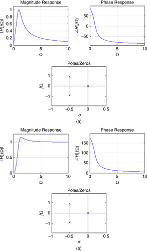
Use MATLAB to find and plot the poles and zeros and the corresponding magnitude and phase frequency responses of:
(a) A second-order band-pass filter and a high-pass filter realized using a series connection of a resistor, an inductor, and a capacitor, each with unit resistance, inductance, and capacitance. Let the input be a voltage source vs(t) and initial conditions be zero.
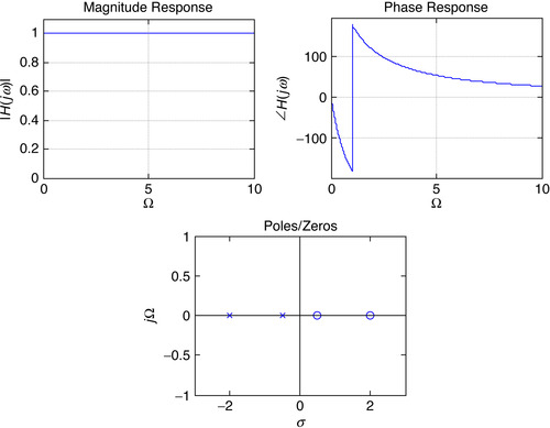
(b) An all-pass filter with a transfer function
Solution
Our function freq resp_s computes and plots the poles and the zeros of the filter transfer function and the corresponding frequency response (the function requests the coefficients of its numerator and denominator in decreasing order of powers of s).
(a) As from a Example 5.16, the transfer functions of the band-pass and high-pass second-order filters are
To compute the frequency response of these filters and to plot their poles and zeros, we used the following script, which uses two functions: freqresp_s, which we give below, and splane, which plots the poles and zeros. The coefficients of the numerator and the denominator correspond to the coefficients, from the highest to the lowest order of s, of the transfer function.
%%%%%%%%%%%%%%%%%%%%%
% Example 5.18---Frequency response
%%%%%%%%%%%%%%%%%%%%%
n = [0 1 0]; % numerator coefficients -- bandpass
% n = [1 0 0]; % numerator coefficients -- highpass
d = [1 1 1]; % denominator coefficients
[w, Hm, Ha] = freqresp_s(n, d, wmax); % frequency response
splane(n, d) % plotting of poles and zeros
The following is the function freqresp_s used to compute the magnitude and phase response of the filter with the given numerator and denominator coefficients.
function [w, Hm, Ha] = freqresp_s(b, a, wmax)
w = 0:0.01:wmax;
H = freqs(b, a, w);
Hm = abs(H); % magnitude
Ha = angle(H) ∗ 180/pi; % phase in degrees
■ Band-pass filter: Letting the output of the filter be the voltage across resistor, we find that the transfer function has a zero at zero, so that the frequency response is zero at Ω = 0. When Ω goes to infinity, one of the two poles cancels the zero effect so that the other pole makes the frequency response tend to zero.
■ High-pass filter: When the output of the filter is the voltage across the inductor the filter is high pass. In this case there is a double zero at s = 0, and the poles are located as before. Thus, when Ω = 0 the magnitude response is zero due to the double zeros at zero, and when Ω goes to infinity the effect of two poles and the two zeros cancel out giving a constant magnitude response, which corresponds to a high-pass filter.
The results for the band-pass and the high-pass filters are shown in Figure 5.11. Notice that the frequency response of the band-pass and the high-pass filter is determined by the ‘number’ of zeros at the origin. The ‘location’ of zeros, like in the all-pass filter we consider next, also determines the frequency response.
(b) All-pass filter: The poles and the zeros of an all-pass filter have the same imaginary parts, but the negative of its real part. At any frequency in the jΩ-axis the lengths of the vectors from the poles equal the length of the vectors from the zeros to the frequency in the jΩ axis. Thus the magnitude response of the filter is unity. The following changes to the above script are needed for the all-pass filter:
clear all
clf
n = [1 −2.5 1];
d = [1 2.5 1];
wmax = 10;
freq_resp_s(n, d, wmax)
The results are shown in Figure 5.12.
5.7.4. Spectrum Analyzer
A spectrum analyzer is a device that measures the spectral characteristics of a signal. It can be implemented as a bank of narrow band band-pass filters with fixed bandwidths covering the desired frequencies (see Figure 5.13). The power at the output of each filter is computed and displayed at the corresponding center frequency. Another possible implementation is using a band-pass filter with an adjustable center frequency, with the power in its bandwidth being computed and displayed [16].
 |
| Figure 5.13 |
If the input of the spectrum analyzer is x(t), the output of either the fixed- or the adjustable-bandpass filters in the implementations—assumed to have a very narrow bandwidth ΔΩ—would be

Computing the mean square of this signal we get
Remarks
■ The bank-of-filter spectrum analyzer is used for the audio range of the spectrum.
■ Radio frequency spectrum analyzers resemble an AM demodulator. It usually consists of a single narrowband intermediate frequency (IF) bandpass filter fed by a mixer. The local oscillator sweeps across the desired band, and the power at the output of the filter is computed and displayed on a monitor.
5.8. Additional Properties
We consider now some additional properties of the Fourier transform, some of which look like those of the Laplace transform when s = jΩ and some are different.
5.8.1. Time Shifting
If x(t) has a Fourier transform X(Ω), then
(5.26)
The Fourier transform of x(t − t0) is

It is important to realize that shifting in time does not change the frequency content of the signal—that is, the signal does not change when delayed or advanced. This is clear when we see that the magnitude of the two transforms, corresponding to the original and the shifted signals, is the same,
Consider the signal
Solution
Applying the time-shift property, we have
Using the duality property, we then have
Consider computing the Fourier transform of y(t) = sin(Ω0t) using the Fourier transform of the cosine signal x(t) = cos(Ω0t) we just found.
5.8.2. Differentiation and Integration
If x(t), −∞ < t < ∞, has a Fourier tranform X(Ω), then
(5.27)
(5.28)


From the inverse Fourier transform given by

The proof of the integration property can be done in two parts:
1. The convolution of u(t) and x(t) gives the integral—that is
(5.29)

2. Since the unit-step signal is not absolutely integrable its Fourier transform cannot be found from the integral definition, and we cannot use its Laplace transform either because its ROC does not include the jΩ axis. Let's transform it into an absolutely integrable signal by subtracting 1/2 and multiplying the result by 2. This gives the sign signal:
(5.30)
(5.31)

Remarks
■ Just like in the Laplace transform where the operator s corresponds to the derivative operation in time of the signal, in the Fourier transform jΩ becomes the corresponding operator for the derivative operation in time of the signal.
Suppose a system is represented by a second-order differential equation with constant coefficients:
Solution
Computing the Fourier transform of this equation, we get

Find the Fourier transform of the triangular pulse
Consider the integral


5.9. What have we Accomplished? What is Next?
You should by now have a very good understanding of the frequency representation of signals and systems. In this chapter, we have unified the treatment of periodic and nonperiodic signals and their spectra, and consolidated the concept of frequency response of a linear time-invariant system.
Basic properties of the Fourier transform and important Fourier pairs are given in Table 5.1 and Table 5.2. Two significant applications are in filtering and communications. We introduced the basics of filtering in this chapter and will expand on them in Chapter 6. The fundamentals of modulation provided in this chapter will be illustrated in Chapter 6 where we will consider their application in communications.
| Function of Time | Function of Ω | |
|---|---|---|
| 1 | δ(t) | 1 |
| 2 | δ(t − τ) | |
| 3 | u(t) | |
| 4 | u(−t) | |
| 5 | ||
| 6 | ||
| 7 | ||
| 8 | ||
| 9 | ||
| 10 | ||
| 11 | ||
| 12 | ||
| 13 | ||
| 14 |
Certainly the next step is to find out where the Laplace and the Fourier analyses apply, which will be done in Chapter 6. After that, we will go into discrete-time signals and systems. We will show that sampling, quantization, and coding bridge the continuous-time and the digital signal processing, and that transformations similar to the Laplace and the Fourier transforms will permit us to do processing of discrete–time signals and systems.
Fourier Series versus Fourier Transform—MATLAB
The connection between the Fourier series and the Fourier transform can be seen by considering what happens when the period of a periodic signal increases to a point at which the periodicity is not clear as only one period is seen. Consider a train of pulses x(t) with a period T0 = 2, and a period of x(t) is x1(t) = u(t + 0.5) − u(t − 0.5). Let T0 be increased to 4, 8, and 16.
(b) Find the Fourier series coefficients for x(t) and carefully plot the magnitude line spectrum for each of the values of T0. Explain what is happening in these spectra.
(c) If you were to let T0 be very large, what would you expect to happen to the Fourier coefficients? Explain.
(d) Write a MATLAB script that simulates the conversion from the Fourier series to the Fourier transform of a sequence of rectangular pulses as the period is increased. The Fourier coefficients need to be multiplied by the period so that they do not become insignificant. Plot using stem the magnitude line spectrum for pulse sequences with periods T0 from 4 to 62.
Fourier Transform from Laplace Transform—MATLAB

The Fourier transform of finite-support signals, which are absolutely integrable or finite energy, can be obtained from their Laplace transform rather than doing the integral. Consider the following signals:
(a) Plot each of the signals.
(b) Find the Fourier transforms {Xi(Ω)} for i = 1, 2, and 3 using the Laplace transform.
(c) Use MATLAB's symbolic function fourier to compute the Fourier transform of the given signals. Plot the magnitude spectrum corresponding to each of the signals.
Fourier Transform from Laplace Transform of Infinite-Support Signals—MATLAB
 and determine whether this signal is absolutely integrable or not.
For signals with infinite support, their Fourier transforms cannot be derived from the Laplace transform unless they are absolutely integrable or the region of convergence of the Laplace transform contains the jΩ axis. Consider the signal  .
.
(a) Plot the signal x(t) for −∞ < t < ∞.
(b) Use the evenness of the signal to find the integral
(c) Use the integral definition of the Fourier transform to find X(Ω).
(d) Use the Laplace transform of x(t) to verify the above found Fourier transform.
(e) Use MATLAB's symbolic function fourier to compute the Fourier transform of x(t). Plot the magnitude spectrum corresponding to x(t).
Fourier and Laplace Transforms—MATLAB
Consider the signal  .
.
(a) Use the fact this signal is bounded by the exponential  to show that the integral
(b) Use the Laplace transform to find the Fourier transform X(Ω) of x(t).
(c) Use the MATLAB function fourier to compute the magnitude and phase spectrum of X(Ω).
Fourier Transform of Causal Signals

Any causal signal x(t) having a Laplace transform with poles in the open-left s-plane (i.e., not including the jΩ axis) has, as we saw before, a region of convergence that includes the jΩ axis, and as such its Fourier transform can be found from its Laplace transform. Consider the following signals:
(a) Determine the Laplace transform of the above signals (use properties of the Laplace transform) indicating the corresponding region of convergence.
(b) Determine for which of these signals you can find its Fourier transform from its Laplace transform. Explain.
(c) Give the Fourier transform of the signals that can be obtained from their Laplace transform.
Duality of Fourier Transform
 or the sinc signal. Its importance is that it is the impulse response of an ideal low-pass filter.
There are some signals for which the Fourier transforms cannot be found directly by either the integral definition or the Laplace transform, and for those we need to use the properties of the Fourier transform, in particular the duality property. Consider, for instance,
(a) Let X(Ω) = A[u(Ω + Ω0) − u(Ω − Ω0] be a possible Fourier transform of x(t). Find the inverse Fourier transform of X(Ω) using the integral equation to determine the values of A and Ω0.
(b) How could you use the duality property of the Fourier transform to obtain X(Ω)? Explain.
Cosine and Sine Transforms
 which is a real function of Ω, thus its computational importance. Show that X(Ω) is also even as a function of Ω.
The Fourier transforms of even and odd functions are very important. The reason is that they are computationally simpler than the Fourier transform. Let  and
and  .
.
(a) Plot x(t) and y(t), and determine whether they are even or odd.
(b) Show that the Fourier transform of x(t) is found from
(c) Find X(Ω) from the above equation (called the cosine transform).
(d) Show that the Fourier transform of y(t) is found from
(e) Find Y(Ω) from the above equation (called the sine transform). Verify that your results are correct by finding the Fourier transform of z(t) = x(t) + y(t) directly and using the above results.
(f) What advantages do you see to the cosine and sine transforms? How would you use the cosine and the sine transforms to compute the Fourier transform of any signal, not necessarily even or odd? Explain.
Time versus Frequency—MATLAB
The supports in time and in frequency of a signal x(t) and its Fourier transform X(Ω) are inversely proportional. Consider a pulse
(a) Let T0 = 1 and T0 = 10 and find and compare the corresponding |X(Ω)|.
(b) Use MATLAB to simulate the changes in the magnitude spectrum when T0 = 10k for k = 0, …, 4 for x(t). Compute X(Ω) and plot its magnitude spectra for the increasing values of T0 on the same plot. Explain the results.
Smoothness and Frequency Content—MATLAB

The smoothness of the signal determines the frequency content of its spectrum. Consider the signals
(a) Plot these signals. Can you tell which one is smoother?
(b) Find X(Ω) and carefully plot its magnitude |X(Ω)| versus frequency Ω.
(c) Find Y(Ω)(use the Fourier transform properties) and carefully plot its magnitude |Y(Ω)| versus frequency Ω.
(d) Which one of these two signals has higher frequencies? Can you now tell which of the signals is smoother? Use MATLAB to decide. Make x(t) and y(t) have unit energy. Plot 20 log10 |Y(Ω)| and 20 log10 |X(Ω)| using MATLAB and see which of the spectra shows lower frequencies.
Smoothness and Frequency—MATLAB
Let the signals x(t) = r(t + 1) − 2r(t) + r(t − 1) and y(t) = dx(t)/dt.
(a) Plot x(t) and y(t).
(b) Find X(Ω) and carefully plot its magnitude spectrum. Is X(Ω) real? Explain.
(c) Find Y(Ω)(use properties of Fourier transform) and carefully plot its magnitude spectrum. Is Y(Ω) real? Explain.
(d) Determine from the above spectra which of these two signals is smoother. Use MATLAB to plot 20 log10 |Y(Ω)| and 20 log10 |X(Ω)| and decide. Would you say in general that computing the derivative of a signal generates high frequencies or possible discontinuities?
Integration and Smoothing—MATLAB
 and let
Consider the signal
(a) Plot x(t) and y(t).
(b) Find X(Ω) and carefully plot its magnitude spectrum. Is X(Ω) real? Explain. (Use MATLAB to do the plotting.)
(c) Find Y(Ω) and carefully plot its magnitude spectrum. Is Y(Ω) real? Explain. (Use MATLAB to do the plotting.)
(d) Determine from the above spectra which of these two signals is smoother. Use MATLAB to decide. Would you say that in general by integrating a signal you get rid of higher frequencies, or smooth out a signal?
Duality of Fourier Transforms
As indicated by the derivative property, if we multiply a Fourier transform by (jΩ)N, it corresponds to computing an Nth derivative of its time signal. Consider the dual of this property—that is, if we compute the derivative of X(Ω), what would happen to the signal in the time?
(a) Let x(t) = δ(t − 1) + δ(t + 1). Find its Fourier transform (using properties) X(Ω).
(b) Compute dX(Ω)/dΩ and determine its inverse Fourier transform.
Periodic Functions in Frequency

 Find its Fourier transform Y(Ω) and plot both y(t) and Y(Ω).
The duality property provides interesting results. Consider the signal
(a) Find  and plot both x(t) and X(Ω).
(b) Suppose you then generate a signal
(c) Are y(t) and the corresponding Fourier transform Y(Ω) periodic in time and in frequency? If so, determine their periods.
Sampling Signal
 will be important in the sampling theory later on.
The sampling signal
(a) As a periodic signal of period Ts, express  by its Fourier series.
(b) Determine then the Fourier transform  .
.
(c) Plot  and Δ(Ω) and comment on the periodicity of these two functions.
Piecewise Linear Signals

The derivative property can be used to simplify the computation of some Fourier transforms. Let
(a) Find and plot the second derivative with respect to t of x(t), or y(t) = d2x(t)/dt2.
(b) Find X(Ω) from Y(Ω) using the derivative property.
(c) Verify the above result by computing the Fourier transform X(Ω) directly from x(t) using the Laplace transform.
Periodic Signal-Equivalent Representations
 and as seen in Chapter 4 the Fourier series coefficients of x(t) are found as
  , so that x(t) can also be represented as
Applying the time and frequency shifts it is possible to get different but equivalent Fourier transforms of periodic signals. Assume a period of a periodic signal x(t) of period T0 is x1(t), so that
(a) Find the Fourier transform of the first expression given above for x(t) using the time-shift property.
(b) Find the Fourier transform of the second expression for x(t) using the frequency-shift property.
(c) Compare the two expressions and comment on your results.
Modulation Property

Consider the raised-cosine pulse
(a) Carefully plot x(t).
(b) Find the Fourier transform of the pulse p(t) = u(t + 1) − u(t − 1).
(c) Use the definition of the pulse p(t) and the modulation property to find the Fourier transform of x(t) in terms of  .
.
Solution of Differential Equations
 where x(t) is the input and y(t) the output. If x(t) = u(t) − 2u(t − 1) + u(t − 2):
An analog averager is characterized by the relationship
(a) Find the Fourier transform of the output Y(Ω).
(b) Find y(t) from Y(Ω).
Generalized AM
 and that the message is a sinusoid of frequency Ω0 = 2π, or x(t) = cos(Ω0t).
Consider the following generalization of amplitude modulation where instead of multiplying by a cosine we multiply by a periodic signal with harmonic frequencies much higher than those of the message. Suppose the carrier c(t) is a periodic signal with fundamental frequency Ω0, let's say
(a) Find the AM signal s(t) = x(t)c(t).
(b) Determine the Fourier transform S(Ω).
(c) What would be a possible advantage of this generalized AM system? Explain.
Filter for Half-Wave Rectifier

Suppose you want to design a dc source using a half-wave rectified signal x(t) and an ideal filter. Let x(t) be periodic, T0 = 2, and with a period
(a) Find the Fourier transform X(Ω) of x(t), and plot the magnitude spectrum including the dc and the first three harmonics.
(b) Determine the magnitude and cut-off frequency of an ideal low-pass filter H(jΩ) such that when we have x(t) as its input, the output is y(t) = 1. Plot the magnitude response of the ideal low-pass filter. (For simplicity assume the phase is zero.)
Passive RLC Filters—MATLAB
Consider an RLC series circuit with a voltage source vs(t). Let the values of the resistor, capacitor, and inductor be unity. Plot the poles and zeros and the corresponding frequency responses of the filters with the output the voltage across the
(a) Capacitor
(b) Inductor
(c) Resistor
Indicate the type of filter obtained in each case. Use MATLAB to plot the poles and zeros, the magnitude, and the phase response of each of the filters obtained above.
AM Modulation and Demodulation
 At the receiver, to recover x(t) the sent signal y(t) needs first to be separated from the thousands of other signals. This is done with a band-pass filter with a center frequency equal to the carrier frequency, and the output of this filter then needs to be demodulated.
 and from it determine the frequency response of the low-pass filter G(jΩ) needed to recover x(t). Plot the magnitude response of G(jΩ).
A pure tone x(t) = 4 cos(1000t) is transmitted using an AM communication system with a carrier cos(10,000t). The output of the AM system is
(a) Consider an ideal band-pass filter H(jΩ). Let its phase be zero. Determine its bandwidth, center frequency, and amplitude so we get as its output 10y(t). Plot the spectrum of x(t), 10y(t), and the magnitude frequency response of H(jΩ).
(b) To demodulate 10y(t), we multiply it by cos(10,000t). You need then to pass the resulting signal through an ideal low-pass filter to recover the original signal x(t). Plot the spectrum of
Ideal Low-Pass Filter—MATLAB

Consider an ideal low-pass filter H(s) with zero phase and magnitude response
(a) Find the impulse response h(t) of the low-pass filter. Plot it and indicate whether this filter is a causal system or not.
(c) Use symbolic MATLAB to find h(t), g(t), and G(jΩ). Plot |H(jΩ)|, h(t), g(t), and |G(jΩ)|.
Magnitude Response from Poles and Zeros—MATLAB
 Use MATLAB to plot the magnitude responses of these filters and indicate the type of filters they are.
Consider the following filters with the given poles and zeros and dc constant:
Different Types of AM Modulations—MATLAB
 be the message or input to different types of AM systems with the output the following signals. Carefully plot m(t) and the following outputs in 0 ≤ t ≤ 1 and their corresponding spectra using MATLAB. Let the sampling period be Ts = 0.001.
Let the signal
(a) y1(t) = m(t) cos(20π t)
(b) y2(t) = [1 + m(t)] cos(20π t)
Windows—MATLAB
The signal x(t) in Problem 5.17 is called a raised-cosine window. Notice that it is a very smooth signal and that it decreases at both ends. The rectangular window is the signal y(t) = u(t + 1) − u(t − 1).
(a) Use MATLAB to compute the magnitude spectrum of x(t) and y(t) and indicate which is the smoother of the two by considering the presence of high frequencies as an indication of roughness.
(b) When computing the Fourier transform of a very long signal it makes sense to break it up into smaller sections and compute the Fourier transform of each. In such a case, windows are used to smooth out the transition from one section to the other. Consider a sinusoid z(t) = cos(2π t) for 0 ≤ t ≤ 1000 sec. Divide the signal into two sections of duration 500 sec. Multiply the corresponding signal in each of the sections by a raised-cosine x(t) and rectangular y(t) windows of length 500 and compute using MATLAB the corresponding Fourier transforms. Compare them to the Fourier transform of the whole signal and comment on your results. Sample all the signals using Ts = 1/(4π) as the sampling period.
(c) Consider the computation of the Fourier transform of the acoustic signal corresponding to a train whistle, which MATLAB provides as a sampled signal in “train.mat” using the discrete approximation of the Fourier transform. The frequency content of the whole signal (hard to find) would not be as meaningful as the frequency content of a smaller section of it as they change with time. Compute the Fourier transform of sections of 1000 samples by windowing the signal with the raised-cosine window (sampled with the same sampling period as the “train.mat” signal or Ts = 1/Fs where Fs is the sampling frequency given for “train.mat”). Plot the spectra of a few of these segments and comment on the change in the frequency content as time changes.
..................Content has been hidden....................
You can't read the all page of ebook, please click here login for view all page.