
Chapter 7. Sampling Theory
The pure and simple truth is rarely pure and never simple.
Oscar Wilde (1854–1900) Irish writer and poet
7.1. Introduction
Since many of the signals found in applications such as communications and control are analog, if we wish to process these signals with a computer it is necessary to sample, quantize, and code them to obtain digital signals. Once the analog signal is sampled in time, the amplitude of the obtained discrete-time signal is quantized and coded to give a binary sequence that can be either stored or processed with a computer.
The main issues considered in this chapter are:
■ How to sample—As we will see, it is the inverse relation between time and frequency that provides the solution to the problem of preserving the information of an analog signal when it is sampled. When sampling an analog signal one could choose an extremely small value for the sampling period so that there is no significant difference between the analog and the discrete signals—visually as well as from the information content point of view. Such a representation would, however, give redundant values that could be spared without losing the information provided by the analog signal. If, on the other hand, we choose a large value for the sampling period, we achieve data compression but at the risk of losing some of the information provided by the analog signal. So how do we choose an appropriate value for the sampling period? The answer is not clear in the time domain. It does become clear when considering the effects of sampling in the frequency domain: The sampling period depends on the maximum frequency present in the analog signal. Furthermore, when using the correct sampling period the information in the analog signal will remain in the discrete signal after sampling, thus allowing the reconstruction of the original signal from the samples. These results, introduced by Nyquist and Shannon, constitute the bridge between analog and discrete signals and systems and were the starting point for digital signal processing as a technical area.
■ Practical aspects of sampling—The device that samples, quantizes, and codes an analog signal is called an analog-to-digital converter (ADC), while the device that converts digital signals into analog signals is called a digital-to-analog converter (DAC). These devices are far from ideal and thus some practical aspects of sampling and reconstruction need to be considered. Besides the possibility of losing information by choosing too large of a sampling period, the ADC also loses information in the quantization process. The quantization error is, however, made less significant by increasing the number of bits used to represent each sample. The DAC interpolates and smooths out the digital signal, converting it back into an analog signal. These two devices are essential in the processing of continuous-time signals with computers.
7.2. Uniform Sampling
The first step in converting a continuous-time signal x(t) into a digital signal is to discretize the time variable—that is, to consider samples of x(t) at uniform times t = nTs, or
(7.1)
7.2.1. Pulse Amplitude Modulation
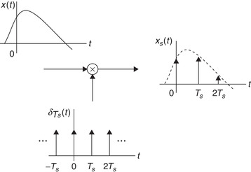
A PAM system can be visualized as a switch that closes every Ts seconds for Δ seconds, and remains open otherwise. The PAM signal is thus the multiplication of the continuous-time signal x(t) by a periodic signal p(t) consisting of pulses of width Δ, amplitude 1/Δ, and period Ts. Thus, xPAM(t) consists of narrow pulses with the amplitudes of the signal within the pulse width. For a small pulse width Δ, the PAM signal is approximately a train of pulses with amplitudes x(mTs)—that is,
(7.2)
Now, as a periodic signal we represent p(t) by its Fourier series
7.2.2. Ideal Impulse Sampling
Given that the pulse width Δ is much smaller than Ts, p(t) can be replaced by a periodic sequence of impulses of period Ts (see Figure 7.1) or  . This simplifies considerably the analysis and makes the results easier to grasp. Later in the chapter we consider the effects of having pulses instead of impulses, a more realistic assumption.
The sampling function , or a periodic sequence of impulses of period Ts, is
(7.3)

(7.4)
There are two equivalent ways to view the sampled signal xs(t) in the frequency domain:
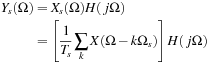
■ Modulation: Since  is periodic, of fundamental frequency Ωs = 2π/Ts, its Fourier series is
(7.5)
(7.6)
■ Discrete-time Fourier transform: The Fourier transform of the sum representation of xs(t) in the second equation in Equation (7.4) is
(7.7)
Remarks
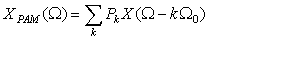
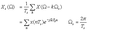
■ The spectrum Xs(Ω) of the sampled signal, according toEquation (7.6), is a superposition of shifted analog spectra {X(Ω − kΩs)} multiplied by 1/Ts(i.e., the modulation process involved in the sampling).
■ Considering that the output of the sampler displays frequencies that are not present in the input, according to the eigenfunction property the sampler is not LTI. It is a time-varying system. Indeed, if sampling x(t) gives xs(t), sampling x(t − τ) where τ ≠ kTsfor an integer k will not be xs(t − τ). The sampler is, however, a linear system.
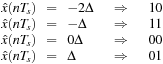
■ Equation (7.7)provides the relation between the continuous frequency Ω(rad/sec) of x(t) and the discrete frequency ω (rad) of the discrete-time signal x(nTs) or x[n] 1:
1To help the reader visualize the difference between a continuous-time signal, which depends on a continuous variable t, or a real number, and a discrete-time signal, which depends on the integer variable n, we will use square brackets for these. Thus, η(t) is a continuous-time signal, while ρ[n] is a discrete-time signal.
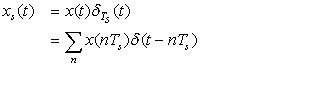
Sampling a continuous-time signal x(t) at uniform times {nTs} gives a sampled signal
(7.8)
(7.9)
If X(Ω) is the Fourier transform of x(t), the Fourier transform of the sampled signal xs(t) is given by the equivalent expressions
(7.10)
Depending on the maximum frequency present in the spectrum of x(t) and on the chosen sampling frequency Ωs(or the sampling period Ts) it is possible to have overlaps when the spectrum of x(t) is shifted and added to obtain the spectrum of the sampled signal. We have three possible situations:
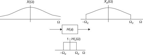
■ If the signal has a low-pass spectrum of finite support—that is, X(Ω) = 0 for |Ω| > Ωmax(seeFigure 7.2(a)) where Ωmaxis the maximum frequency present in the signal—such a signal is called band limited. As shown inFigure 7.2(b), for band-limited signals it is possible to choose Ωsso that the spectrum of the sampled signal consists of shifted nonoverlapping versions of (1/Ts)X(Ω). Graphically (seeFigure 7.2(b)), this can be accomplished by letting Ωs − Ωmax ≥ Ωmax, or
■ On the other hand, if the signal x(t) is band limited but we let Ωs < 2Ωmax, then when creating Xs(Ω) the shifted spectra of x(t) overlap (seeFigure 7.2(c)). In this case, due to the overlap it will not bepossible to recover the original continuous-time signal from the sampled signal, and thus the sampled signal does not share the same information with the original continuous-time signal. This phenomenon is called frequency aliasing since due to the overlapping of the spectra some frequency components of the original continuous-time signal acquire a different frequency value or an “alias.”
■ When the spectrum of x(t) does not have a finite support (i.e., the signal is not band limited) sampling using any sampling period Tsgenerates a spectrum of the sampled signal consisting of overlapped shifted spectra of x(t). Thus, when sampling non-band-limited signals frequency aliasing is always present. The only way to sample a non-band-limited signal x(t) without aliasing—at the cost of losing information provided by the high-frequency components of x(t) — is by obtaining an approximate signal xa(t) that lacks the high-frequency components of x(t), thus permitting us to determine a maximum frequency for it. This is accomplished by antialiasing filtering commonly used in samplers.
 |
| Figure 7.2 |

Consider the signal x(t) = 2 cos(2πt + π/4), −∞ < t < ∞. Determine if it is band limited or not. Use Ts = 0.4, 0.5, and 1 sec/sample as sampling periods, and for each of these find out whether the Nyquist sampling rate condition is satisfied and if the sampled signal looks like the original signal or not.
Solution
Since x(t) only has the frequency 2π, it is band limited with Ωmax = 2π rad/sec. For any Ts the sampled signal is given as
(7.13)

Using Ts = 0.4 sec/sample the sampling frequency in rad/sec is Ωs = 2π/Ts = 5π > 2Ωmax = 4π, satisfying the Nyquist sampling rate condition. The samples in Equation (7.13) are then
 |
| Figure 7.3 |
When Ts = 0.5 the sampling frequency is Ωs = 2π/Ts = 4π = 2Ωmax, barely satisfying the Nyquist sampling rate condition. The samples in Equation (7.13) are now
We use MATLAB to plot the continuous signal and four sampled signals (see Figure 7.3) for different values of Ts. Clearly, when Ts = 1 sec/sample there is no similarity between the analog and the discrete signals due to frequency aliasing.
(a)
(b) 
Solution
(a) The signal x1(t) = u(t + 0.5) − u(t − 0.5) is a unit pulse signal. Clearly, this signal can be easily sampled by choosing any value of Ts << 1. For instance, Ts = 0.01 sec would be a good value, giving a discrete-time signal x1(nTs) = 1, for 0 ≤ nTs = 0.01n ≤ 1 or 0 ≤ n≤ 100. There seems to be no problem in sampling this signal; however, we have that the Fourier transform of x1(t),
Using Parseval's energy relation we have that the energy of x1(t) (the area under  ) is 1 and if we wish to find a value ΩM, such that 99% of this energy is in the frequency band [−ΩM, ΩM], we need to look for the limits of the following integral so it equals 0.99:

%%%%%%%%%%%%%%%%%%%%%
% Example 7.2 --- Parseval's relation and sampling
%%%%%%%%%%%%%%%%%%%%%
syms W
for k = 1:23;
E(k) = int((sin(0.5*W)/(0.5*W))^2,0,k*pi)/pi
if E(k)> = 0.9900,
k
return
end
end
(b) For the causal exponential

7.2.3. Reconstruction of the Original Continuous-Time Signal
If the signal x(t) to be sampled is band limited with Fourier transform X(Ω) and maximum frequency Ωmax, by choosing the sampling frequency Ωs to satisfy the Nyquist sampling rate condition, or Ωs > 2Ωmax, the spectrum of the sampled signal xs(t) displays a superposition of shifted versions of the spectrum of x(t), multiplied by 1/Ts, but with no overlaps. In such a case, it is possible to recover the original analog signal from the sampled signal by filtering. Indeed, if we consider an ideal low-pass analog filter  with magnitude Ts in the pass-band −Ωs/2 < Ω < Ωs/2, and zero elsewhere—that is,
(7.14)
Bandlimited or Not?
The following, taken from David Slepian's paper “On Bandwidth”[66], clearly describes the uncertainty about bandlimited signals:
The Dilemma—Are signals really bandlimited? They seem to be, and yet they seem not to be.
On the one hand, a pair of solid copper wires will not propagate electromagnetic waves at optical frequencies and so the signals I receive over such a pair must be bandlimited. In fact, it makes little physical sense to talk of energy received over wires at frequencies higher than some finite cutoff W, say 1020 Hz. It would seem, then, that signals must be bandlimited.
On the other hand, however, signals of limited bandwith W are finite Fourier transforms, and irrefutable mathematical arguments show them to be extremely smooth. They possess derivatives of all orders. Indeed, such integrals are entire functions of t, completely predictable from any little piece, and they cannot vanish on any t interval unless they vanish everywhere. Such signals cannot start or stop, but must go on forever. Surely real signals start and stop, and they cannot be bandlimited!
Thus we have a dilemma: to assume that real signals must go on forever in time (a consequence of bandlimitedness) seems just as unreasonable as to assume that real signals have energy at arbitrary high frequencies (no bandlimitation). Yet one of these alternatives must hold if we are to avoid mathematical contradiction, for either signals are bandlimited or they are not: there is no other choice. Which do you think they are?
Remarks
■ In practice, the exact recovery of the original signal may not be possible for several reasons. One could be that the continuous-time signal is not exactly band limited, so that it is not possible to obtain a maximum frequency causing frequency aliasing in the sampling. Second, the sampling is not done exactly at uniform times—random variation of the sampling times may occur. Third, the filter required for the exact recovery is an ideal low-pass filter, which in practice cannot be realized; only an approximation is possible. Although this indicates the limitations of sampling, in most cases where: (1) the signal is band limited or approximately band limited, (2) the Nyquist sampling rate condition is satisfied in the sampling, and (3) the reconstruction filter approximates well the ideal low-pass filter, the recovered signal closely approximates the original signal.
■ For signals that do not satisfy the band-limitedness condition, one can obtain an approximate signal that satisfies that condition. This is done by passing the non-band-limited signal through an ideal low-pass filter. The filter output is guaranteed to have as maximum frequency the cut-off frequency of the filter (seeFigure 7.4). Because of the low-pass filtering, the filtered signal is a smoothed version of the original signal—high frequencies of the signal have been removed. The low-pass filter is called an antialiasing filter, since it makes the approximate signal band limited, thus avoiding aliasing in the frequency domain.
■ In applications, the cut-off frequency of the antialiasing filter is set according to prior knowledge. For instance, when sampling speech, it is known that speech has frequencies ranging from about 100 Hz toabout 5 KHz (this range of frequencies provides understandable speech in phone conversations). Thus, when sampling speech an anti-aliasing filter with a cut-off frequency of 5 KHz is chosen and the sampling rate is then set to 10,000 samples/sec. Likewise, it is also known that an acceptable range of frequencies from 0 to 22 KHz provides music with good fidelity, so that when sampling music signals the anti-aliasing filter cut-off frequency is set to 22 KHz and the sampling rate to 44K samples/sec or higher to provide good-quality music.
Origins of the Sampling Theory—Part 1
The sampling theory has been attributed to many engineers and mathematicians. It seems as if mathematicians and researchers in communications engineering came across these results from different perspectives. In the engineering community, the sampling theory has been attributed traditionally to Harry Nyquist and Claude Shannon, although other famous researchers such as V. A. Kotelnikov, E. T. Whittaker, and D. Gabor came out with similar results. Nyquist's work did not deal directly with sampling and reconstruction of sampled signals but it contributed to advances by Shannon in those areas.
Harry Nyquist was born in Sweden in 1889 and died in 1976 in the United States. He attended the University of North Dakota at Grand Forks and received his Ph.D. from Yale University in 1917. He worked for the American Telephone and Telegraph (AT&T) Company and the Bell Telephone Laboratories, Inc. He received 138 patents and published 12 technical articles. Nyquist's contributions range from the fields of thermal noise, stability of feedback amplifiers, telegraphy, and television, to other important communications problems. His theoretical work on determining the bandwidth requirements for transmitting information provided the foundations for Claude Shannon's work on sampling theory [33].
As Hans D. Luke [44] concludes in his paper “The Origins of the Sampling Theorem,” regarding the attribution of the sampling theorem to many authors:
This history also reveals a process which is often apparent in theoretical problem in technology or physics: first the practicians put forward a rule of thumb, then theoreticians develop the general solution, and finally someone discovers that the mathematicians have long since solved the mathematical problem which it contains, but in “splendid isolation.”
Consider the two sinusoids

Solution
Sampling the two signals using Ts = 2π/Ωs, we have


%%%%%%%%%%%%%%%%%%%%%%%%%%%%%%%%%%%%%%%%%
% Example 7.3 --- Two sinusoids of different frequencies being sampled
% with same sampling period -- aliasing for signal with higher frequency
clear all; clf
% sinusoids
omega_0 = 1;omega_s = 7;
T = 2 ∗ pi/omega_0; t = 0:0.001:T; % a period of x1
x1 = cos(omega_0 ∗ t); x2 = cos((omega_0 + omega_s) ∗ t);
N = length(t); Ts = 2 ∗ pi/omega_s; % sampling period
M = fix(Ts/0.001); imp = zeros(1,N);
for k = 1:M:N − 1.
imp(k) = 1; % sequence of impulses
end
xs = imp.∗ x1; % sampled signal
plot(t,x1,'b',t,x2,'k'), hold on
stem(t,imp. ∗ x1,'r','filled'),axis([0 max(t)− 1.1 1.1]); xlabel('t'), grid
Figure 7.5 shows the two sinusoids and the sampled signal that coincides for the two signals. The result in the frequency domain is shown in Figure 7.6: The spectra of the two sinusoids are different but the spectra of the sampled signals are identical.
 |
| Figure 7.5 |

7.2.4. Signal Reconstruction from Sinc Interpolation
The analog signal reconstruction from the samples can be shown to be an interpolation using sinc signals. First, the ideal low-pass filter  in Equation (7.14) has as impulse response
(7.15)

(7.16)

7.2.5. Sampling Simulation with MATLAB
The simulation of sampling with MATLAB is complicated by the representation of analog signals and the numerical computation of the analog Fourier transform. Two sampling rates are needed: one being the sampling rate under study, fs, and the other being the one used to simulate the analog signal, fsim >> fs. The computation of the analog Fourier transform of x(t) can be done approximately using the fast Fourier transform (FFT) multiplied by the sampling period. For now, think of the FFT as an algorithm to compute the Fourier transform of a discretized signal.
To illustrate the sampling procedure consider sampling a sinusoid x(t) = cos(2πf0t) where f0 = 1 KHz. To simulate this as an analog signal we choose a sampling period Tsim = 0.5 × 10⁻⁴ sec/sample or a sampling frequency fsim = 20,000 samples/sec.
No aliasing sampling—If we sample x(t) with a sampling frequency fs = 6000 > 2 f0 = 2000 Hz, the sampled signal y(t) will not display aliasing in its frequency representation, as we are satisfying the Nyquist sampling rate condition. Figure 7.7(a) displays the signal x(t) and its sampled version y(t), as well as their approximate Fourier transforms. The magnitude spectrum |X(Ω)| corresponds to the sinusoid x(t), while |Y(Ω)| is the first period of the spectrum of the sampled signal (recall the spectrum of the sampled signal is periodic of period Ωs = 2πfs). In this case, when no aliasing occurs, the first period of the spectrum of y(t) coincides with the spectrum of x(t) (notice that as a sinusoid, the magnitude spectrum |X(Ω)| is zero except at the frequency of the sinusoid or ±1 KHz; likewise |Y(Ω)| is zero except at ±1 KHz and the range of frequencies is [−fs/2, fs/2] = [−3, 3] KHz). In Figure 7.7(b) we show the sinc interpolation of three samples of y(t); the solid line is the interpolated values or the sum of sincs centered at the three samples. At the bottom of that figure we show the sinc interpolation, for all the samples, obtained using our function sincinterp. The sampling is implemented using our function sampling.
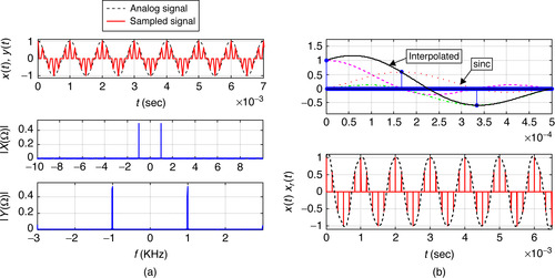
Sampling with aliasing—In Figure 7.8 we show the case when the sampling frequency is fs = 800 < 2fs = 2000, so that in this case we have aliasing. This can be seen in the sampled signal y(t) in the top plot of Figure 7.8(a), which appears as if we were sampling a sinusoid of lower frequency. It can also be seen in the spectra of x(t) and y(t): |X(Ω)| is the same as in the previous case, but now |Y(Ω)|, which is a period of the spectrum of the sampled signal y(t), displays a frequency of 200 Hz, lower than that of x(t), within the frequency range [−400, 400] Hz or [−fs/2, fs/2]. Aliasing has occurred. Finally, the sinc interpolation gives a sinusoid of frequency 0.2 KHz, different from x(t).

Similar situations occur when a more complex signal is sampled. If the signal to be sampled is x(t) = 2 − cos(πf0t) − sin(2πf0t) where f0 = 500 Hz, if we use a sampling frequency of fs = 6000 > 2 fmax = 2 f0 = 1000 Hz, there will be no aliasing. On the other hand, if the sampling frequency is fs = 800 < 2fmax = 2f0 = 1000 Hz, frequency aliasing will occur. In the no aliasing sampling, the spectrum |Y(Ω)| (in a frequency range [−3000, 3000] = [−fs/2, fs/2]) corresponding to a period of the Fourier transform of the sampled signal y(t) shows the same frequencies as |X(Ω)|. The reconstructed signal equals the original signal. See Figure 7.9(a). When we use fs = 800 Hz, the given signal x(t) is undersampled and aliasing occurs. The spectrum |Y(Ω)| corresponding to a period of the Fourier transform of the undersampled signal y(t) does not show the same frequencies as |X(Ω)|. The reconstructed signal shown in the bottom right plot of Figure 7.9(b) does not resemble the original signal.
 |
| Figure 7.9 |
The following function implements the sampling and computes the Fourier transform of the analog signal and of the sampled signal using the fast Fourier transform. It gives the range of frequencies for each of the spectra.
function [y,y1,X,fx,Y,fy] = sampling(x,L,fs)
%
%Sampling
%x analog signal
%L length of simulated x
%fs sampling rate
%y sampled signal
%X,Y magnitude spectra of x,y
%fx,fy frequency ranges for X,Y
%
fsim = 20000; % analog signal sampling frequency
% sampling with rate fsim/fs
delta = fsim/fs;
y1 = zeros(1,L);
y = x(1:delta:L);
% analog FT and DTFT of signals
dtx = 1/fsim;
X = fftshift(abs(fft(x))) ∗ dtx;
N = length(X); k = 0:(N− 1); fx = 1/N.*k; fx = fx ∗ fsim/1000− fsim/2000;
dty = 1/fs;
Y = fftshift(abs(fft(y))) ∗ dty;
N = length(Y); k = 0:(N− 1); fy = 1/N.*k; fy = fy∗ fs/1000− fs/2000;
The following function computes the sinc interpolation of the samples.
function [t,xx,xr] = sincinterp(x,Ts)
%
% Sinc interpolation
% x sampled signal
% Ts sampling period of x
% xx,xr original samples and reconstructed in range t
%
N = length(x)
t = 0:dT:N;
xr = zeros(1,N ∗ 100 + 1);
for k = 1:N,
end
xx(1:100:N ∗ 100) = x(1:N);
xx = [xx zeros(1,99)];
NN = length(xx)
t = 0:NN− 1;t = t ∗ Ts/100;
7.3. The Nyquist-Shannon Sampling Theorem
If a low-pass continuous-time signal x(t) is band limited (i.e., it has a spectrum X(Ω) such that X(Ω) = 0 for |Ω| > Ωmax, where Ωmax is the maximum frequency in x(t)), we then have:
■ x(t) is uniquely determined by its samples  , n = 0, ±1, ±2, ⋯, provided that the sampling frequency Ωs (rad/sec) is such that
(7.17)
(7.18)
■ When the Nyquist sampling rate condition is satisfied, the original signal x(t) can be reconstructed by passing the sampled signal xs(t) through an ideal low-pass filter with the following frequency response:
(7.19)
Remarks
■ The value 2Ωmaxis called the Nyquist sampling rate. The value Ωs/2 is called the folding rate.
■ The units of the sampling frequency fsare samples/sec and as such the units of Tsare sec/sample. Considering the number of samples available, every second or the time at which each sample is available we can get a better understanding of the data storage requirements, the speed limitations imposed by real-time processing, and the need for data compression algorithms. For instance, music being sampled at 44,000 samples/sec, with each sample represented by 8 bits/sample, for every second of music we would need to store 44 × 8 = 352 Kbits/sec, and in an hour of sampling we would have 3600 × 44 × 8 Kbits. If you want better quality, let's say 16 bits/sample, then double that quantity, and if you want more fidelity increase the sampling rate but be ready to provide more storage or to come up with some data compression algorithm. Likewise, if you were to process the signal you would have a new sample every Ts = 0.0227 msec, so that any real-time processing would have to be done very fast.
Origins of the Sampling Theory — Part 2
As mentioned in Chapter 0, the theoretical foundations of digital communications theory were given in the paper “A Mathematical Theory of Communication” by Claude E. Shannon in 1948 [51]. His results on sampling theory made possible the new areas of digital communications and digital signal processing.
Shannon was born in 1916 in Petoskey, Michigan. He studied electrical engineering and mathematics at the University of Michigan, pursued graduate studies in electrical engineering and mathematics at MIT, and then joined Bell Telephone Laboratories. In 1956, he returned to MIT to teach.
Besides being a celebrated researcher, Shannon was an avid chess player. He developed a juggling machine, rocket-powered frisbees, motorized Pogo sticks, a mind-reading machine, a mechanical mouse that could navigate a maze, and a device that could solve the Rubik's Cube™ puzzle. At Bell Labs, he was remembered for riding the halls on a unicycle while juggling three balls 23 and 52.
7.3.1. Sampling of Modulated Signals
The given Nyquist sampling rate condition applies to low-pass or baseband signals. Sampling of band-pass signals is used for simulation of communication systems and in the implementation of modulation systems in software radio. For modulated signals it can be shown that the sampling rate depends on the bandwidth of the message or modulating signal, not on the absolute frequencies involved. This result provides a significant savings in the sampling, as it is independent of the carrier. A voice message transmitted via a satellite communication system with a carrier of 6 GHz, for instance, would only need to be sampled at about a 10-KHz rate, rather than at 12 GHz as determined by the Nyquist sampling rate condition when we consider the frequencies involved.
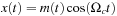
Consider a modulated signal x(t) = m(t) cos(Ωct) where m(t) is the message and cos(Ωct) is the carrier with carrier frequency
If the message m(t) of a modulated signal x(t) = m(t) cos(Ωc) has a bandwidth B Hz, x(t) can be reconstructed from samples taken at a sampling rate
Consider the development of an AM transmitter that uses a computer to generate the modulated signal and is capable of transmitting music and speech signals. Indicate how to implement the transmitter.
Solution
Let the message be m(t) = x(t)+ y(t) where x(t) is a speech signal and y(t) is a music signal. Since music signals display larger frequencies than speech signals, the maximum frequency of m(t) is that of the music signals, or fmax = 22 KHz. To transmit m(t) using AM, we modulate it with a sinusoid of frequency fc > fmax, say fc = 3fmax = 66 KHz.
To satisfy the Nyquist sampling rate condition, the maximum frequency of the modulated signal would be fc + fmax = (66 +2 2) KHz = 88 KHz, and so we would choose Ts = 10−3/176 sec/sample as the sampling period. However, according to the above results we can also choose Ts = 1/(2B) where B is the bandwidth of m(t) in hertz or B = fmax = 22 KHz, which gives Ts = 10−3/44 — four times larger than the previous sampling period, so we choose this as the sampling period.
The analog signal m(t) to be transmitted is inputted into an ADC in the computer, capable of sampling at 44, 000 samples/sec. The output of the converter is then multiplied by a computer-generated sinusoid
7.4. Practical Aspects of Sampling
To process analog signals with computers it is necessary to convert analog into digital signals and digital into analog signals. The analog-to-digital and digital-to-analog conversions are done by ADCs and DACs. In practice, these converters differ from the ideal versions we have discussed so far where the sampling is done with impulses, the discrete-time samples are assumed representable with infinite precision, and the reconstruction is performed by an ideal low-pass filter. Pulses rather than impulses are needed, and the discrete-time signals need to be discretized also in amplitude and the reconstruction filter needs to be reconsidered.
7.4.1. Sample-and-Hold Sampling
In an actual ADC the time required to do the sampling, quantization, and coding needs to be considered. Therefore, the width Δ of the sampling pulses cannot be zero as assumed. A sample-and-hold sampling system takes the sample and holds it long enough for quantization and coding to be done before the next sample is acquired. The question is then how does this affect the sampling process and how does it differ from the ideal results obtained before? We hinted at the effects when we considered the PAM before, except that now the resulting pulses are flat.
The system shown in Figure 7.10 generates the desired signal. Basically, we are modulating the ideal sampling signal  with the analog input x(t), giving an ideally sampled signal xs(t). This signal is then passed through a zero-order hold filter, an LTI system having as impulse response h(t) a pulse of the desired width Δ ≤ Ts. The output of the sample-and-hold system is a weighted sequence of shifted versions of the impulse response. In fact, the output of the ideal sampler is
  , and using the linearity and time invariance of the zero-order hold system its output is
(7.20)
(7.21)
(7.22)


Remarks
■Equation (7.20)can be written as
■ The spectrum of the ideal sampled signal xs(t) is now weighted by the sinc function of the frequency response H(jΩ) of the zero-order hold filter. Thus, the spectrum of the sampled signal using the sample-and-hold system will not be periodic and will decay as Ω increases.
■ The reconstruction of the original signal x(t) requires a more complex filter than the one used in the ideal sampling. Indeed, the concatenation of the zero-order hold filter with the reconstruction filter should be such that H(s)Hr(s) = 1, or that Hr(s) = 1/H(s).
■ A circuit used for implementing the sample-and-hold system is shown inFigure 7.11. In this circuit the switch closes every Tsseconds and remains closed for a short time Δ. If the time constant rC << Δ, the capacitor charges very fast to the value of the sample attained when the switch closes at some nTs, and by setting the time constant RC >> Tswhen the switch opens Δ seconds later, the capacitor slowly discharges. The cycle repeats providing a signal that approximates the output of the sample-and-hold system explained before.

■ The DAC also uses a holder to generate an analog signal from the discrete signal coming out of the decoder into the DAC. There are different possible types of holders, providing an interpolation that will make the final smoothing of the signal a lot easier. The so-called zero-order hold basically expands the sample value in between samples, providing a rough approximation of the discrete signal, which is then smoothed out by a low-pass filter to provide the analog signal.
7.4.2. Quantization and Coding
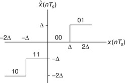
Amplitude discretization of the sampled signal xs(t) is accomplished by a quantizer consisting of a number of fixed amplitude levels against which the sample amplitudes {x(nTs)} are compared. The output of the quantizer is one of the fixed amplitude levels that best represents x(nTs) according to some approximation scheme. The quantizer is a nonlinear system.
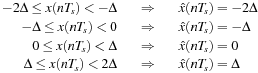
Independent of how many levels, or equivalently of how many bits are allocated to represent each level of the quantizer, there is a possible error in the representation of each sample. This is called the quantization error. To illustrate this, consider a 2-bit or 22-level quantizer shown in Figure 7.12. The input of the quantizer are the samples x(nTs), which are compared with the values in the bins [−2Δ, −Δ], [−Δ, 0], [0, Δ], and [Δ, 2Δ], and depending on which of these bins the sample falls in it is replaced by the corresponding levels −2Δ, −Δ, 0, or Δ. The value of the quantization step Δ for the four-level quantizer is
(7.23)
To see the quantization, coding, and quantization error, let the sampled signal be
(7.24)
If we define the quantization error as
(7.25)
In practice, the quantization error is considered random, and so it needs to be characterized probabilistically. This characterization becomes meaningful only when the number of bits is large, and the input signal is not a deterministic signal. Otherwise, the error is predictable and thus not random. Comparing the energy of the input signal to the energy of the error, by means of the so-called signal-to-noise ratio (SNR), it is possible to determine the number of bits that are needed in a quantizer to get a reasonable quantization error.
Suppose we are trying to decide between an 8- and a 9-bit ADC for a certain application. The signals in this application are known to have frequencies that do not exceed 5 KHz. The amplitude of the signals is never more than 5 volts (i.e., the dynamic range of the signals is 10 volts, so that the signal is bounded as −5 ≤ x(t) ≤ 5). Determine an appropriate sampling period and compare the percentage of error for the two ADCs of interest.
Solution
The first consideration in choosing the ADC is the sampling period, so we need to get an ADC capable of sampling at fs = 1/Ts > 2fmax samples/sec. Choosing fs = 4fmax = 20 K samples/sec, then Ts = 1/20 msec/sample. Suppose then we look at an 8-bit ADC, which means that the quantizer would have 28 = 256 levels so that the quantization step is Δ = 10/256 volts. If we use the truncation quantizer given above the quantization error would be
7.4.3. Sampling, Quantizing, and Coding with MATLAB
The conversion of an analog signal into a digital signal consists of three steps: sampling, quantization, and coding. These are the three operations an ADC does. To illustrate them consider a sinusoid x(t) = 4 cos(2πt). Its sampling period, according to the Nyquist sampling rate condition, is
 |
| Figure 7.13 |
% Sampling, quantization and coding
%%%%%%%%%%%%%%%%%%%%%%%%%%%
clear all; clf
% analog signal
t = 0:0.01:1; x = 4 ∗ sin(2 ∗ pi ∗ t);
% sampled signal
Ts = 0.01; N = length(t); n = 0:N − 1;
xs = 4 ∗ sin(2 ∗ pi ∗ n ∗ Ts);
% quantized signal
Q = 2;% quantization levels is 2Q
[d,y,e] = quantizer(x,Q);
% binary signal
z = coder(y,d)
The quantization of the sampled signal is implemented with the function quantizer which compares each of the samples xs(nTs) with four levels and assigns to each the corresponding level. Notice the appproximation of the values given by the quantized signal samples to the actual values of the signal. The difference between the original and the quantized signal, or the quantization error, ε(nTs), is also computed and shown in Figure 7.13.
function [d,y,e] = quantizer(x,Q)
% Input: x, signal to be quantized at 2Q levels
% Outputs: y quantized signal
%e, quantization error
%d quantum
% USE [d,y,e] = quantizer(x,Q)
%
N = length(x);
d = max(abs(x))/Q;
for k = 1:N,
if x(k)>= 0,
y(k) = floor(x(k)/d)*d;
else
if x(k) == min(x),
y(k) = (x(k)/abs(x(k))) ∗(floor(abs(x(k))/d) ∗ d);
else
y(k) = (x(k)/abs(x(k))) ∗ (floor(abs(x(k))/d) ∗ d + d);
end
end
if y(k) == 2 ∗ d,
y(k) = d;
end
end
The binary signal corresponding to the quantized signal is computed using the function coder which assigns the binary codes '10','11','00', and '01' to the four possible levels of the quantizer. The result is a sequence of 0s and 1s, each pair of digits sequentially corresponding to each of the samples of the quantized signal. The following is the function used to effect this coding.
function z1 = coder(y,delta)
% Coder for 4-level quantizer
% input: y quantized signal
% output: z1 binary sequence
% USE z1 = coder(y)
%
z1 = '00'; % starting code
N = length(y);
for n = 1:N,
y(n)
if y(n) == delta
z = '01';
elseif y(n) == 0
z = '00';
elseif y(n) == -delta
z = '11';
else
z = '10';
end
z1 = [z1 z];
end
M = length(z1);
z1 = z1(3:M) % get rid of starting code
7.5. What Have We Accomplished? Where Do We Go from Here?
The material in this chapter is the bridge between analog and digital signal processing. The sampling theory provides the necessary information to convert a continuous-time signal into a discrete-time signal and then into a digital signal with minimum error. It is the frequency representation of an analog signal that determines the way in which it can be sampled and reconstructed. Analog-to-digital and digital-to-analog converters are the devices that in practice convert an analog signal into a digital signal and back. Two parameters characterizing these devices are the sampling rate and the number of bits each sample is coded into. The rate of change of a signal determines the sampling rate, while the precision in representing the samples determines the number of levels of the quantizer and the number of bits assigned to each sample.
In the following chapters we will consider the analysis of discrete-time signals, as well as the analysis and synthesis of discrete systems. The effect of quantization in the processing and design of systems is an important problem that is left for texts in digital signal processing. We will, however, develop the theory of discrete-time signals.
Sampling Actual Signals
Consider the sampling of real signals.
(a) Typically, a speech signal that can be understood over a telephone shows frequencies from about 100 Hz to about 5 KHz. What would be the sampling frequency fs (samples/sec) that would be used to sample speech without aliasing? How many samples would you need to save when storing an hour of speech? If each sample is represented by 8 bits, how many bits would you have to save for the hour of speech?
(b) A music signal typically displays frequencies from 0 up to 22 KHz. What would be the sampling frequency fs that would be used in a CD player?
(c) If you have a signal that combines voice and musical instruments, what sampling frequency would you use to sample this signal? How would the signal sound if played at a frequency lower than the Nyquist sampling frequency?
Sampling of Band-Limited Signals
Consider the sampling of a sinc signal and related signals.
(a) For the signal x(t) = sin(t)/t, find its magnitude spectrum |X(Ω)| and determine if this signal is band limited or not.
(b) Suppose you want to sample x(t)). What would be the sampling period Ts you would use for the sampling without aliasing?
(c) For a signal y(t) = x2(t), what sampling frequency fs would you use to sample it without aliasing? How does this frequency relate to the sampling frequency used to sample x(t)?
(d) Find the sampling period Ts to sample x(t) so that the sampled signal xs(0) = 1, otherwise xs(nTs) = 0 for n ≠ 0.
Sampling of Time-Limited Signals—MATLAB
Consider the signals x(t) = u(t) − u(t − 1) and y(t) = r(t) − 2r(t − 1) + r(t − 2).
(a) Are either of these signals band limited? Explain.
(b) Use Parseval's theorem to determine a reasonable value for a maximum frequency for these signals (choose a frequency that would give 90% of the energy of the signals). Use MATLAB.
(c) If we use the sampling period corresponding to y(t) to sample x(t), would aliasing occur? Explain.
(d) Determine a sampling period that can be used to sample both x(t) and y(t) without causing aliasing in either signal.
Uncertainty in Time and Frequency—MATLAB
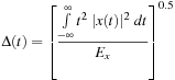 measures the duration of the signal for which the signal is significant in time, and
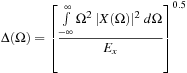 measures the frequency support for which the Fourier representation is significant. The energy of the signal is represented by Ex. Compute Δ(t) and Δ(Ω) for the given signal x(t) and verify that the uncertainty principle is satisfied.
Signals of finite time support have infinite support in the frequency domain, and a band-limited signal has infinite time support. A signal cannot have finite support in both domains.
(a) Consider x(t) = (u(t + 0.5) − u(t − 0.5))(1 + cos(2πt)). Find its Fourier transform X(Ω). Compute the energy of the signal, and determine the maximum frequency of a band-limited approximation signal  that would give 95% of the energy of the original signal.
(b) The fact that a signal cannot be of finite support in both domains is expressed well by the uncertainty principle, which says that
Nyquist Sampling Rate Condition and Aliasing

Consider the signal
(a) Find the Fourier transform X(Ω) of x(t).
(b) Is x(t) band limited? If so, find its maximum frequency Ωmax.
(c) Suppose that Ts = 2π. How does Ωs relate to the Nyquist frequency 2Ωmax? Explain.
(d) What is the sampled signal x(nTs) equal to? Carefully plot it and explain if x(t) can be reconstructed.
Anti-Aliasing

Suppose you want to find a reasonable sampling period Ts for the noncausal exponential
(a) Find the Fourier transform of x(t), and plot |X(Ω)|. Is x(t) band limited?
(b) Find a frequency Ω0 so that 99% of the energy of the signal is in −Ωo ≤ Ω ≤ Ωo.
(c) If we let Ωs = 2π/Ts = 5Ω0, what would be Ts?
(d) Determine the magnitude and bandwidth of an anti-aliasing filter that would change the original signal into the band-limited signal with 99% of the signal energy.
Sampling of Modulated Signals
 where m(t) is the message signal and Ωc = 2π104 rad/sec is the carrier frequency.
Assume you wish to sample an amplitude modulated signal
(a) If the message is an acoustic signal with frequencies in a band of [0, 22] KHz, what would be the maximum frequency present in x(t)?
(b) Determine the range of possible values of the sampling period Ts that would allow us to sample x(t) satisfying the Nyquist sampling rate condition.
(c) Given that x(t) is a band-pass signal, compare the above sampling period with the one that can be used to sample band-pass signals.
Sampling Output of Nonlinear System
 where x(t) is the input and y(t) is the output.
The input–output relation of a nonlinear system is
(a) The signal x(t) is band limited with a maximum frequency ΩM = 2000π rad/sec. Determine if y(t) is also band limited, and if so, what is its maximum frequency Ωmax?
(b) Suppose that the signal y(t) is low-pass filtered. The magnitude of the low-pass filter is unity and the cut-off frequency is Ωc = 5000π rad/sec. Determine the value of the sampling period Ts according to the given information.
(c) Is there a different value for Ts that would satisfy the Nyquist sampling rate condition for both x(t) and y(t) and that is larger than the one obtained above? Explain.
Signal Reconstruction
You wish to recover the original analog signal x(t) from its sampled form x(nTs).
(a) If the sampling period is chosen to be Ts = 1 so that the Nyquist sampling rate condition is satisfied, determine the magnitude and cut-off frequency of an ideal low-pass filter H(jΩ) to recover the original signal and plot them.
(b) What would be a possible maximum frequency of the signal? Consider an ideal and a nonideal low-pass filter to reconstruct x(t). Explain.
CD Player versus Record Player
Explain why a CD player cannot produce the same fidelity of music signals as a conventional record player. (If you do not know what these are, ignore this problem, or get one to find out what they do or ask your grandparents about LPs and record players!)
Two-Bit Analog-to-Digital Converter—MATLAB

 where x(nTs), found above, is the input and
  is the output of the quantizer. Let the quantization step be Δ = 0.5. Plot the input–output characterization of the quantizer, and find the quantized output for each of the sample values of the sampled signal x(nTs).
 Obtain the digital signal corresponding to x(t).
Let x(t) = 0.8 cos(2πt) + 0.15, 0 ≤ t ≤ 1, and zero otherwise, be the input to a 2-bit analog-to-digital converter.
(a) For a sampling period Ts = 0.025 sec determine and plot using MATLAB the sampled signal,
(b) The four-level quantizer (see Figure 1.2) corresponding to the 2-bit ADC is defined as
(7.26)
(c) To transform the quantized values into unique binary 2-bit values, consider the following code:
..................Content has been hidden....................
You can't read the all page of ebook, please click here login for view all page.