
Mining Software Logs for Goal-Driven Root Cause Analysis
Hamzeh Zawawy*; Serge Mankovskii†; Kostas Kontogiannis‡; John Mylopoulos§ * Department of Electrical & Computer Engineering, University of Waterloo, Waterloo, ON, Canada
† CA Labs, San Francisco, CA, USA
‡ Department of Electrical and Computer Engineering, National Technical University of Athens, Athens, Greece
§ Department of Information Engineering and Computer Science, University of Trento, Trento, Italy
Abstract
Root cause analysis for software systems is a challenging diagnostic task owing to the complex interactions between system components, the sheer volume of logged data, and the often partial and incomplete information available for root cause analysis purposes. This diagnostic task is usually performed by human experts who create mental models of the system at hand, generate root cause hypotheses, conduct log analysis, and identify the root causes of an observed system failure. In this chapter, we discuss a root cause analysis framework that is based on goal and antigoal models to represent the relationship between a system behavior or requirement, and the necessary conditions, configurations, properties, constraints, or external actions that affect this particular system behavior. We consequently use these models to generate a Markov logic network that allows probabilistic reasoning, so that conclusions can be reached even with incomplete or partial data and observations. The proposed framework improves on existing approaches by handling uncertainty in observations, using natively generated log data, and by being able to provide ranked diagnoses. The framework is evaluated using a sample application based on commercial off-the-shelf software components.
18.1 Introduction
Software root cause analysis is the process by which system operators attempt to identify faults that have caused system application failures. By failure we mean any deviation of the system’s observed behavior from the expected one, while by fault we refer to a software bug or system misconfiguration. For systems that comprise a large number of components that encompass complex interactions, the root cause analysis process may require a large volume of data to be logged, collected, and analyzed. It has been argued in the literature that the increase in the number of services/systems in a distributed environment can directly contribute to the increase of its overall complexity and the effort required to maintain it [1]. It has also been estimated that 40% of large organizations collect more than 1 TB of log data per month, and 11% of them collect more than 10 TB of log data monthly [2]. In this context, and in order to maintain the required service quality levels, IT systems must be constantly monitored and evaluated by analyzing complex logged data emanating from diverse components. However, the sheer volume of such logged data often makes manual log analysis impossible, and therefore there is a need to provide tools for automating this task to a large extent.
Nevertheless, there are challenges in automating log analysis for root cause identification. These challenges stem first from the complexity of interdependencies between system components, second from the often incomplete log data for explaining the root cause of a failure, and third from the lack of models that could be used to denote conditions and requirements under which a failure could be manifested. The problem becomes even more complex when the failures are caused not by internal faults, but rather by external actions initiated by third parties.
In this chapter, we present an approach to root cause analysis that is based on the use of requirements models (goal models) to capture cause-effect relationships, and a probabilistic reasoning approach to deal with partial or incomplete log data and observations. More specifically, first we use goal models to denote the conditions, constraints, actions, and tasks a system is expected carry out in order to fulfill its requirements. Similarly, we use antigoal models to denote the conditions, constraints, actions, and tasks that could be taken by an external agent to invalidate or threaten a system’s functional or nonfunctional requirements. Second, we use latent semantic indexing (LSI) as an information retrieval technique in order to reduce the volume of the software logs that can be considered as observations for a given root cause analysis session so that the performance and tractability of the root cause analysis process can be increased. Third, we compile a knowledge base by transforming goal and antigoal models to a collection of weighted Markov logic diagnostic rules. In this context, when a failure is observed, the goal and antigoal models for which their root nodes correspond to the observed failure are analyzed in order to identify the tasks and actions that may explain the observed failure. The confidence for a root cause further increases when both a goal model and an antigoal model support this root cause hypothesis. Confidence levels are computed as part of the Markov logic reasoning process, combined with rule weights learned from past observations, thus providing a level of training in the reasoning process. The material presented in this chapter builds on previous work conducted by the authors [3, 4].
The chapter is organized as follows. Section 18.2 discusses related work in the areas of root cause analysis. Section 18.3, goal models, antigoal models, node annotations, and a running example are presented. Log reduction is discussed in Section 18.5, while reasoning using Markov logic is presented in Section 18.6. In Section 18.7, we describe in detail the framework and its application to detect failures caused by internal system faults. Section 18.8 describes the use of the root cause analysis framework for identifying the root causes of system failures stemming from external actions. In Section 18.9, we present and discuss the experimental results related to applying the framework to both internally and externally caused failures. Finally, Section 18.10 presents a summary and the conclusions of the chapter.
18.2 Approaches to Root Cause Analysis
In principle, root cause analysis approaches can be classified into three main categories: rule-based, probabilistic, and model-based approaches. Some approaches rely on natively generated low-level system traces [5, 6]. Others rely on log data obtained by instrumenting the source code [7], or by intercepting system calls [8]. In the following sections, we outline the main concepts behind each of these approaches.
18.2.1 Rule-Based Approaches
This class of root cause analysis approaches uses rules to capture the domain knowledge of the monitored IT environment. Such rules are typically of the form <If symptoms then diagnosis>, where symptoms are mapped to root causes. This set of rules is built manually by interviewing system administrators, or automatically by using machine learning methods applied on past data. To find the root cause of an incident, the set of rules is evaluated for matching symptoms. When the conditions of a rule are satisfied, the rule is triggered and a conclusion for the root cause of the failure is derived.
In general, the drawback of the rule-based root cause analysis approaches is that it is hard to have a comprehensive set of rules that cover all the possible cases. Furthermore, the overhead work needed before these approaches can be used in practice is not trivial and requires there to be updating for new incidents. In our work we use goal models to represent cause-effect relationships at a higher level of abstraction, as well as probabilistic rules so that reasoning can be performed with partial or incomplete log data.
18.2.2 Probabilistic Approaches
Traditional root cause analysis techniques assume that interdependencies between system components are fully known a priori and that log information about the monitored system’s state is complete for all diagnostic purposes. Probabilistic approaches aim to model the cause and effect relationships between IT components using probabilities to represent the possible effect of one component on another. An example of using the probabilistic approach is the work of Steinder et al. [9]. They used Bayesian networks to represent dependencies between communication systems and diagnose failures while using dynamic, missing, or inaccurate information about the system structure and state.
Another example is the approach of Al-Mamory et al. [10], who used a history of alarms and resolutions in order to improve future root cause analysis. In particular, they used root cause analysis to reduce the large number of alarms by finding the root causes of false alarms. The approach uses data mining to group similar alarms into generalized alarms and then analyzes these generalized alarms and classifies them into true and false alarms.
18.2.3 Model-Based Approaches
This class of root cause analysis techniques aims at compiling a model representing the normal behavior of the system, and detecting anomalies when the monitored behavior does not adhere to the model. Such models denoting the normal behavior of a system can take various forms. One form is to associate design decisions and components with functional and nonfunctional system properties. For example, these associations can be represented by goal models, antigoal models, or i*-diagrams. A system that uses model-driven engineering combined with run-time information for facilitating root cause analysis is presented in Ref. [11]. More specifically, models denoting system behavior and structure are used to annotate the source code at design time. At run time, logged data are compared with design-time models in order to infer possible root causes. Similarly, a model-based approach facilitating root cause analysis for business process compliance is presented in Ref. [12]. The system allows the specification of models denoting business processes, as well as constraints on/policies for these processes. A run-time monitoring infrastructure allows the collection of system events that are consequently analyzed against the constraints and the policies in the model repository. The analysis yields possible violations, as well as the causes of these violations. Linear temporal logic models were used in Ref. [13] to represent business process compliance constraints in complex service-oriented systems. Symptoms are associated with causes by utilizing current reality trees. An analysis engine allows the current reality trees to be traversed when a symptom is observed, evaluate whether a constraint is violated, and establish possible causes of this violation. Another example of model-based approaches is given in Ref. [7], and is based on the propositional satisfaction of system properties using SAT solvers. Given a propositional formula f, the propositional satisfiability (SAT) problem consists in finding values for the variables of the propositional formula that can make an overall propositional formula evaluate to true. The propositional formula is said to be true if such a truth assignment exists. In Ref. [7] effects (i.e., symptoms or requirement violations) are linked to causes using goal trees. Consequently, goal trees are transformed to propositional formulas. The objective of root cause analysis when a symptom is observed is to identify which combination of goal nodes (i.e., causes) could support or explain the observed violation. One way of solving this problem is by utilizing SAT solvers applied in the logic formula that stems from the goal tree.
18.3 Root Cause Analysis Framework Overview
As illustrated in Figure 18.1, the root cause analysis framework consists of three phases: modeling, observation generation, and diagnostics. The first phase is an off-line preparatory phase. In this phase, system administrators generate a set of models to represent the requirements of the monitored applications. For this, we use goal and antigoal models (discussed in Section 18.4) as a formalism of choice to represent the monitored applications. Goal models and antigoal models are transformed to collections of rules, forming a diagnostic rule base. Goal and antigoal model nodes are annotated with additional information that represents precondition, postcondition, and occurrence constraints for each of these nodes. The second phase of the framework starts when an alarm is raised indicating the monitored application has failed. In this phase (discussed in Section 18.5), the goal model that corresponds to the observed failed requirement is triggered and its node annotations are used to extract a reduced event set from the logged data. This event set is used, along with the goal and antigoal models, to build a fact base of observations. In the third phase of the framework (discussed in Section 18.6), a reasoning process that is based on Markov logic networks (MLNs) is applied to identify root causes from the diagnostic knowledge base. The overall behavior of the proposed framework is outlined in the sequence diagram depicted in Figure 18.2.


18.4 Modeling Diagnostics for Root Cause Analysis
18.4.1 Goal Models
Goal models are tree structures that can be used to represent and denote the conditions and the constraints under which functional and nonfunctional requirements of a system can be delivered. In these structures, internal nodes represent goals, while external nodes (i.e., leafs) represent tasks. Edges between nodes represent either AND or OR goal decompositions or contributions.
The AND decomposition of a goal G into other goals or tasks C1, C2, …, Cn implies that the satisfaction of each of G’s children is necessary for the decomposed goal to be fulfilled. The OR decomposition of a goal G into other goals or tasks C1, C2, …, Cn implies that the satisfaction of one of these goals or tasks suffices for the satisfaction of the parent goal. In Figure 18.3, we show goals g1 and g3 as examples of AND and OR decompositions.

In addition to AND/OR decompositions, two goals may be connected by a contribution edge. A goal may potentially contribute to other goals in four ways—namely, ++S, −−S, ++D and −−D. In this chapter, we adopt the semantics of Chopra et al. [14] for the interpretations of contributions:

18.4.2 Antigoal Models
Similarly to goal models, antigoal models represent the goals and actions of an external agent with the intention to threaten or compromise specific system goals. Antigoal models are also denoted as AND/OR trees built through systematic refinement, until leaf nodes (i.e., tasks) are derived. More specifically, leaf nodes represent tasks (actions) an external agent can perform to fulfill an antigoal, and consequently through the satisfaction of this antigoal to deny a system goal. In this respect, root cause analysis can commence by considering root causes not only due to internal system faults but also due to external actions. Antigoal models were initially proposed by Lamsweerde et al. [15] to model security concerns during requirements elicitation.
An example of antigoal models is the trees with roots ag1 and ag2, depicted in Figure 18.3, where the target edges from antigoal ag1 to tasks a2 and a3 as well as from antigoal ag2 to tasks a4 and a6 model the negative impact an antigoal has on a system goal.
18.4.3 Model Annotations
Since a generic goal model is only an abstract description of cause and effect relationships, it is not sufficient on its own to capture whether goals are satisfied on the basis of input from the collected log data. For this reason, we consider three annotations per goal or task node: precondition, postcondition, and occurrence annotations. Precondition annotations denote the structure and contents the log data must have at a particular (logical) time instant for the goal or task be considered for evaluation. Occurrence annotations denote the structure and contents the log data must have at a particular (logical) time instant for the goal to be considered potentially satisfiable. Similarly, postcondition annotations denote the structure and contents the log data must have at a particular (logical) time instant for the goal to be tagged as satisfied. The order of logical time instants and the logical relationship between preconditions, occurrence and postconditions for a given goal or task are presented in Equations 18.9-18.12 for goal models, and Equations 18.17 and 18.18 for antigoal models.
Goal and task node annotations pertaining to preconditions, occurrence, and postconditions take the form of expressions as discussed in Section 18.7.1.2 and illustrated in Equation 18.10. Figure 18.3 depicts an example of annotating goal model nodes with precondition, postcondition, and occurrence expressions. Once goal and antigoal models have been formulated and annotated, they are consequently transformed into collections of Markov logic rules in order to form a diagnostic knowledge base, as will be discussed in the following sections.
In addition to assisting in inferring whether a goal or action node is satisfied, annotations serve as a means for reducing, through information retrieval approaches, the volume of the logs to be considered for the satisfaction of any given node, increasing the overall root cause analysis processing performance. Logs are filtered on a per goal node basis using the metadata annotation information in each node. Log reduction uses LSI and is discussed in more detail in Section 18.5. Other approaches to log reduction that are based on information theory were proposed in Ref. [16]. The reduced logs that are obtained from the running system are also transformed to collections of facts, forming a fact base of observations. The rule base stemming from the goal and antigoal models and the facts stemming from the observed log files form a complete knowledge base to be used for root cause analysis reasoning. Root cause analysis reasoning uses a probabilistic rule engine that is based on the Alchemy tool [17]. In the following sections we discuss in more detail log filtering, reasoning fundamentals using Markov logic, and the application of the framework used for root cause analysis for (a) failures that occur because of internal system errors and (b) failures that occur as a result of external actions.
18.4.4 Loan Application Scenario
Throughout this chapter, as a running example to better illustrate the inner workings of the proposed root cause analysis technique, we use example goal and antigoal models pertaining to a loan application scenario as depicted in Figure 18.3. The scenario is built on a test environment that is composed of a set of COTS application components. As depicted in Figure 18.4, the experimentation environment includes a business process layer and a service-oriented infrastructure. In particular, this test environment includes four subsystems: the front-end application (SoapUI), a middleware message broker, a credit check service, and a database server.

We have built the Apply_For_Loan business service, specifying the process of an online user applying for a loan, having the loan application evaluated, and finally obtaining an accept/reject decision based on the information supplied. Technically, the business process is exposed as a Web service. The Apply_For_Loan service starts when it receives a SOAP request containing loan application information. It evaluates the loan request by checking the applicant’s credit rating. If the applicant’s credit rating is “good,” his/her loan application is accepted and a positive reply is sent to the applicant. Otherwise, a loan rejection result is sent to the applicant. If an error occurs during processing, a SOAP fault is sent to the requesting application. The credit rating evaluation is performed via a separate Web service (Credit_Rating). After the credit evaluation terminates, the Credit_Rating service sends a SOAP reply to the calling application containing the credit rating and the ID of the applicant. If an error occurs during the credit evaluation, a SOAP error is sent to the requesting application. During the credit rating evaluation, the Credit_Rating application queries a database table and stores/retrieves the applicants’ details.
18.4.4.1 Goal model for the motivating scenario
The loan application is represented by the goal model in Figure 18.3, which contains three goals (rectangles) and seven tasks (circles). The root goal g1 (loan application) is AND-decomposed to goal g2 (loan evaluation) and tasks a1 (eeceive loan Web service request) and a2 (send loan Web service reply), indicating that goal g1 is satisfied if and only if goal g2 and tasks a1 and a2 are satisfied. Similarly, g2 is AND-decomposed to goal g3 (extract credit rating) and tasks a3 (receive credit check Web service request), a4 (update loan table), and a5 (send credit Web service reply), indicating that goal g2 is satisfied if and only if goal g3 and tasks a3, a4, and a5 are satisfied. Furthermore, subgoal g3 is OR-decomposed into tasks a6 and a7. This decomposition indicates that goal g3 is satisfied if either task a6 or task a7 is satisfied. Contribution links (++D) from goal g3 to tasks a4 and a5 indicate that if goal g3 is denied, then tasks a4 and a5 should be denied as well. Contribution link (++S) from goal g2 to task a1 indicates that if goal g2 is satisfied, then so must be task a1. Table 18.1 provides a complete list of the goals and tasks in the loan application goal model. We will discuss the role of antigoals ag1 and ag2 later in the chapter.
Table 18.1
Loan Application Goal Model’s Node/Precondition/Postcondition Identifiers
| Node | Precondition | Postcondition |
| g1 | InitialReq_Submit | Reply_Received |
| g2 | ClientInfo_Valid | Decision_Done |
| a1 | BusinessProc_Ready | BusProc_Start |
| a2 | LoanRequest_Submit | LoanRequest_Avail |
| a3 | Decision_Done | LoanReply_Ready |
| a4 | SOAPMessage_Avail | SOAPMessage_Sent |
| a5 | ClientInfo_Valid | Prepare_CreditRating_Request |
| a6 | Prepare_CreditRating_Request | Receive_CreditRating_Rply |
| a7 | Receive_CreditRating_Rply | Valid_CreditRating |
| a8 | Valid_CreditRating | CreditRating_Available |
| a9 | CreditRating_Available | Decision_Done |
18.4.4.2 Logger systems in the test environment
The test environment includes four logging systems that emit log data. The logging systems we have used include the following:
1. Windows Event Viewer: This is a Windows component that acts as a Windows centralized log repository. Events emanating from applications running as Windows services (middleware and database server) can be accessed and viewed using the Windows Event Viewer.
2. SoapUI: This is an open source Web service testing tool for service- oriented architecture. SoapUI logs its events in a local log file.
3. Web Service logger: This corresponds to the Credit_Rating application, and generates events that are stored directly in the log database.
18.5 Log Reduction
Log reduction pertains to a process that allows the selection of a subset of the available logs to be used for root cause analysis purposes. The motivation is that by reducing the size of the log files (i.e., the number of events to be considered), we can make root cause analysis more tractable and efficient with respect to its time performance. However, such a reduction has to keep entries important to the analysis, while discarding irrelevant ones, thus maintaining a high recall and high precision for the results obtained. The basic premise used here for log reduction is that each log entry represents a document, while terms and keywords obtained from the goal and antigoal model node annotations are treated as queries. The documents (i.e., log entries) that conform with the query form then the reduced set. Here, we discuss the background techniques which we use to reduce the size of the logged data to be considered for the satisfaction of each goal model node, and that thus make the whole process more tractable. More specifically, we consider LSI and probabilistic latent semantic indexing (PLSI) as two techniques used to discover relevant documents (i.e., log entries) given keywords in a query (i.e., keywords and terms obtained by annotations in goal model nodes related to the analysis). A detailed discussion on how annotations are used for log reduction is presented in Section 18.7.1.2.
18.5.1 Latent Semantic Indexing
Some of the well-known document retrieval techniques include LSI [18], PLSI [19], latent Dirichlet allocation [20], and the correlated topic model [21]. In this context, semantic analysis of a corpus of documents consists in building structures that identify concepts from this corpus of documents without any prior semantic understanding of the documents.
LSI is an indexing and retrieval method to identify relationships among terms and concepts in a collection of unstructured text documents. LSI was introduced by Deerwester et al. [18]. It takes a vector space representation of documents based on term frequencies as a starting point and applies a dimension reduction operation on the corresponding term/document matrix using the singular value decomposition algorithm [22]. The fundamental idea is that documents and terms can be mapped to a reduced representation in the so-called latent semantic space. Similarities among documents and queries can be more efficiently estimated in this reduced space representation than in their original representation. This is because two documents which have terms that have been found to frequently co-occur in the collection of all documents will have a similar representation in the reduced space representation, even if these two specific documents have no terms in common. LSI is commonly used in areas such as Web retrieval, document indexing [23], and feature identification [24]. In this context, we consider each log entry as a document. The terms found in the goal and antigoal node annotation expressions become the search keywords. LSI is then used to identify those log entries that are mostly associated with a particular query denoting a system feature, a precondition, an occurrence, or a postcondition annotation of a goal or antigoal node.
18.5.2 Probabilistic Latent Semantic Indexing
PLSI is a variation of LSI [19] that considers the existence of three types of random variables (topic, word, and document). The three types of class variables are as follows:
(1) An unobserved class variable z ∈ Z = {z1,z1,...zK} that represents a topic
(2) Word w ∈ W = {w1,w2,...wL}, where each word is the location of a term t from the vocabulary V in a document d
(3) Document d ∈ D = {d1,d2,...dM} in a corpus M
PLSI aims to identify the documents di in a collection of documents {d1, d2, .., dj} that best relate to a word w (or words), presented as query—that is, to compute P(di,w). The major difference of PLSI from LSI is that its model is based on three layers—namely, the documents layer, the latent topics layer, and the words (i.e., query) layer. Each document di is associated with one or more concepts ck (i.e., a latent variable). Similarly, each word is also associated with a concept. The overall objective is to compute the conditional probabilities P(ck|di) and P(w|ck). By computing the inner product of P(w|ck) and P(di|ck) over latent variables ck for each document d in the collection of documents separately, as the “similarity” score between the query w and a document di, we can then select the documents that produce the maximum score. Such documents are considered as the most relevant to the query.
18.6 Reasoning Techniques
As discussed in Section 18.4, we use goal models to represent dependencies between system requirements and design decisions, components, and system properties. Each goal model is represented as a goal tree. The root of the tree represents a functional or a nonfunctional requirement for the given system. When a failure is observed (i.e., a failure to observe the delivery of a functional or nonfunctional requirement), the corresponding goal tree is analyzed. Goal models are transformed to first-order logic formulas so that a SAT solver or a reasoning engine can determine the assignment of truth values to the nodes of the tree in a way that explains the failure of the requirement that corresponds to the root node of the goal or antigoal tree. However, to evaluate the actual truth value of each node we would require that the node annotations are evaluated using observations (i.e., events) and information found in the system logs as presented in Sections 18.7.1.4, 18.7.1.6, and 18.8.1. In practical situations though, observations can be missing, erroneous, or considered as valid within a degree of likelihood or probability. For this reason, we resort to the use of a probabilistic reasoning engine to cope with uncertain, erroneous, or missing observations. In this section, we discuss such a probabilistic reasoning technique that we use, and that is based on the Markov logic theory [17].
18.6.1 Markov Logic Networks
MLNs were recently proposed in the research literature as a framework that combines first-order logic and probabilistic reasoning. In this context, a knowledge base denoted by first-order logic formulas represents a set of hard constraints on the set of possible worlds (i.e., if a world violates one formula, it has zero probability of existing). Markov logic softens these constraints by making a word that violates a formula be less probable, but still possible. The more formulas it violates, the less probable it becomes. A detailed discussion on MLNs can be found in Ref. [25].
Markov network construction. In MLNs, each logic formula Fi is associated with a nonnegative real-valued weight wi. Every grounding (instantiation) of Fi is given the same weight wi. In this context, a Markov network is an undirected graph that is built by an exhaustive grounding of the predicates and formulas as follows:
• Each node corresponds to a ground atom xk which is an instantiation of a predicate.
• If a subset of ground atoms x{i} = {xk} are related to each other by a formula Fi with weight wi, then a clique Ci over these variables is added to the network. Ci is associated with a weight wi and a feature function fi defined as follows:

Thus, first-order logic formulas serve as templates to construct the Markov network. In the context of a Markov network, each ground atom, X, represents a binary variable. The overall Markov network is then used to model the joint distribution of all ground atoms. The corresponding global energy function can be calculated as follows:

where Z is the normalizing factor calculated as

where i denotes the subset of ground atoms x{i}∈ X that are related to each other by a formula Fi with weight wi and feature function fi.
Learning. Learning in an MLN consists of two steps: structure learning, or learning the logical clauses, and weight learning, or determining the weight of each logical clause. Structure learning is typically done by heuristically searching the space for models that have a statistical score measure that fits the training data [17]. As for weight learning, Singla et al. [26] extended the existing voted perceptron method and applies it to generate the MLN’s parameters (weights for the logical clauses). This is done by optimizing the conditional likelihood of the query atoms given the evidence.
Inference, Assuming ϕi(x{i}) is the potential function defined over a clique Ci, then ![]() . We use the Markov network constructed to compute the marginal distribution of events. Given some observations, probabilistic inference can be performed. Exact inference is often intractable, and thus Markov chain Monte Carlo sampling techniques, such as Gibbs sampling, are used for approximate reasoning [25]. The probability for an atom Xi given its Markov blanket (neighbors) Bi is calculated as follows:
. We use the Markov network constructed to compute the marginal distribution of events. Given some observations, probabilistic inference can be performed. Exact inference is often intractable, and thus Markov chain Monte Carlo sampling techniques, such as Gibbs sampling, are used for approximate reasoning [25]. The probability for an atom Xi given its Markov blanket (neighbors) Bi is calculated as follows:
where


Fi is the set of all cliques that contain Xi, and fj is computed as in Equation 18.2.
The Markov network is used to compute the marginal distribution of events and perform inference. Because inference in Markov networks is #P-complete, approximate inference is proposed to be performed using the Markov chain Monte Carlo method and Gibbs sampling [27].
As already mentioned, the above expressions are used to compute the probability an atom X (i.e., an instantiated predicate in one of the logic formulas stemming from the goal models) belongs to a clique in the Markov network. Intuitively, this probability gives the likelihood this atom is satisfied in the “world” represented by the clique. As an example, consider the first-order logic formula ![]() . If we have atoms A and B, then we can infer C exists. But if we consider that we have seen a “world” where B and C coexist on their own in 40% of cases without A, then even in the absence of observing A, we can still deduce C exists with a degree of likelihood if we observe B alone without A. In the sections below, we elaborate more on the use of probabilistic reasoning for root cause analysis for failures due to internal system errors or due to external maliciously induced actions.
. If we have atoms A and B, then we can infer C exists. But if we consider that we have seen a “world” where B and C coexist on their own in 40% of cases without A, then even in the absence of observing A, we can still deduce C exists with a degree of likelihood if we observe B alone without A. In the sections below, we elaborate more on the use of probabilistic reasoning for root cause analysis for failures due to internal system errors or due to external maliciously induced actions.
18.7 Root Cause Analysis for Failures Induced by Internal Faults
In this section, we present the elements of the probabilistic-based root cause analysis framework and we illustrate its use through the loan application example. The framework consists of three main components: system modeling, observation generation, and diagnosis. This framework takes as input, first, the set of annotated goal models that represent the monitored systems and, second, the log data stored in unified format in a centralized database. It generates as output a ranked list of diagnostics that represents the weighted possible root cause(s) of the failure.
18.7.1 Knowledge Representation
In the following sections, we discuss in more detail the steps pertaining to modeling a diagnostic knowledge base from a collection of goal models.
18.7.1.1 Goal model compilation
The root cause analysis framework is built on the premise that the monitored system’s requirements goal model is available to system analysts or can be reverse engineered from source code using techniques discussed in Ref. [28]. Tasks in a goal model represent simple components in the source code. These are treated as black boxes for the purposes of monitoring and diagnosis in order to enable us to model a software system at different levels of abstraction.
18.7.1.2 Goal model annotations
We extend the goal models representing the monitored systems by annotating the goal model nodes with additional information. In particular, tasks (leaf nodes) are associated with preconditions, occurrence, and postconditions, while goals (nonleaf nodes) are associated with preconditions and postconditions only. The annotations are expressed using string pattern expressions of the form [not]column_name[not]like“match_string″, where column_name represents a field name in the log database and match_string can contain the following symbols:
• %: matches strings of zero or many characters;
• _ (underscore): matches one character;
• [...]: encloses sets or ranges, such as [abc] or [a − d].
An annotation example is the precondition for goal g1 (in Figure 18.3) shown below:
Pre(g1): Description like ’%starting%Database%eventsDB%’ AND source:component like ‘eventsDB’
This annotation example matches events containing keywords or attribute values indicating that they have been generated by the “eventsDB” database system, and have a description text or attribute values containing the keyword “starting,” followed by a space, then followed by the keyword “Database,” then a space, followed by the keyword “eventsDB.” More annotation examples are shown in Figure 18.3.
18.7.1.3 Goal model predicates
We use first-order logic to represent semantic information on goal and antigoal models. More specifically, we represent the monitored systems/services’ states and actions as first-order logic predicates. A predicate is intentional if its truth value can only be inferred (i.e., it cannot be directly observed). A predicate is extensional if its truth value can be observed directly. A predicate is strictly extensional if it can only be observed and not inferred for all its groundings [29]. We use the extensional predicates ChildAND(parent_node,child_node) and ChildOR(parent_node,child_node) to denote the AND/OR goal decomposition. For instance, ChildAND(parent,child) is true when child is an AND-child of parent (similarly for ChildOR(parent,child)). Examples of AND goal decomposition are goals g1 and g2 shown in Figure 18.3. An example of OR decomposition is goal g3. We use the extensional predicates Pre(node,timestep), Occ(node,timestep), and Post(node,timestep) to represent preconditions, task occurrences, and task postconditions at a certain timestep. For our work, we assume a total ordering of events according to their logical or physical timestamps [30]. The predicate Satisfied is predominantly intentional except for the top goal for which satisfaction is observable (i.e., the observed system failure that triggers the root cause analysis process). If the overall service/transaction is successfully executed, then the top goal is considered to be satisfied, otherwise it is denied.
18.7.1.4 Goal model rules
The satisfaction of goals, antigoals, and tasks is expressed using the truth assignment of the Satisfied(node, timestep) predicate, which, in turn, are inferred as follows: A task a with a precondition {Pre} and a postcondition {Post} is satisfied at time t + 1 if and only if {Pre} is true at time t − 1 just before task a occurs at time t, and {Post} is true at time t + 1 as follows:
The satisfaction of the Pre(task,timestep) and Post(task,timestep) predicates is based on whether there are events or event patterns that match the node annotations tagged as Pre, Occ, or Post, for the given task node.
Annotation expressions are string patterns linked by logical operators of the form

where column name represents a field name in the log database, and the search pattern string contains symbols such as % (percent), which matches strings of zero or more characters, and _ (underscore), which matches one character.
The following is an annotation example for the precondition of node a2:
Precond(a2): Description like ’Windows.%starting.up’ AND Source Component like alpha.com.ca’
The satisfaction of the Occ(task,timestep) predicate for leaf nodes is based on the same principles as the satisfaction of the Pre(node,timestep) and Post(node,timestep) predicates as presented above.
Unlike tasks (i.e., the leaf nodes), which occur at a specific moment of time, goal occurrences (i.e., internal nodes) may span an interval [t1, t2] that is based on the satisfaction timesteps of the child goals/tasks. Thus, a goal g with precondition {Pre} and postcondition {Post} is satisfied at time t3 if the goal precondition {Pre} expression is observed at t1, the goal occurrence is observed at timestep t2, and {Post} expression is observed at timestep t3, where (t1<t2<t3) (see Equations 18.11-18.13). The truth values of the predicate Occ(goal, timestep) (used in Equation 18.13) can be inferred only on the basis on the satisfaction of all its children in the case of AND-decomposed goals (Equation 18.11) or at least one of its children in the case of OR-decomposed goals (Equation 18.12).

From the above, the rule for the satisfaction of an internal goal node is given as follows:
Contribution links of the form node1 ![]() node2 are represented in Equation 18.14 (similarly for + +D, −−S, and −−D):
node2 are represented in Equation 18.14 (similarly for + +D, −−S, and −−D):
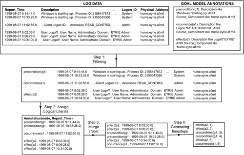
18.7.1.5 Generation of ground atoms from filtered system logs
There are two inputs to this process: first, the log data stored in a common database, and second, the goal model for the monitored system with precondition, postcondition, and occurrence patterns annotating each node of the model. The output is a totally timestep-ordered set of literals (ground atoms) of the form literal(node,timestep).
The framework uses pattern expressions that annotate the goal models and applies these annotations as queries to the log data in order to extract evidence for the occurrence of events associated with each goal model node. More specifically, once the logged data have been stored in a unified format, the pattern expressions that annotate the goal and antigoal model nodes (see Figure 18.3) can be used, first, to generate LSI queries that are applied to collect a subset of the logged data pertaining to the analysis and, second, as patterns to satisfy Pre, Occ, and Post predicates for a node. An example of a log data pattern matching expression for the precondition of goal g1 in Figure 18.3 is shown below:
The truth assignment for the extensional predicates is performed on the basis of the pattern matched log data. We show below a sample subset of the ground atoms for the goal model in Figure 18.3:
pre(g1,1), pre(a1,1), occ(a1,2), post(a1,3), pre(g2,3), !pre(a3,3), ?occ(a3,4), …, ?post(g1,15), !satisfied(g1,15)
The set of literals above represents the observation of one failed loan application session. However, for some of the goals/tasks, there may be no Pre, Occ, or Post supporting evidence, which can be interpreted as either they did not occur, or they were missed from the observation set. We model this uncertainty by adding a question mark (?) before the corresponding ground atoms. In cases where there is evidence that a goal/task did not occur, the corresponding ground atom is preceded by an exclamation mark (!). For example, in Figure 18.3 the observation of the system failure is represented by !satisfied(g1,15), which indicates top goal g1 denial, at timestep 15. Note that in the above example, the precondition for task a3 was denied and the occurrence of a3 was not observed, leading to the denial of task a3, which led to goal g2 not occurring and thus being denied. In turn, the denial of goal g2 supports goal g1 not being satisfied.
The filtering of the predicate with timesteps of interest is performed in two steps. First, a list of literals is generated (see the example above) from the nodes annotations (preconditions, occurrences, and postconditions) by depth-first traversing the goal model tree. In the second step, literals are used to initiate searches in the logged data set looking for events containing such literals (and within a certain time interval). The following is an example of the generation of ground atoms. A log entry of the form
(2010-02-05 17:46:44.24 Starting up database eventsDB ... DATABASE)
that matches the pattern of the precondition of goal g1 represents evidence for the satisfaction of the precondition of g1. For other logical literals that do not have supporting evidence in the log data that their preconditions, postconditions, or occurrence expressions are matched, a question mark is assigned to these literals. Such a case is illustrated in the precondition of of a7 (Occ(a7,5)) in Table 18.2
Table 18.2
Four Scenarios for the Loan Application
| Scenario | Observed (& missing) events | Satisfied (a1,3) | Satisfied (a3,5) | Satisfied (a6,7) | Satisfied (a7,9) | Satisfied (a4,11) | Satisfied (a5,13) | Satisfied (a2,15) |
| 1. Successful execution | Pre(g1,1), Pre(a1,1), Occ(a1,2), Post(a1,3), Pre(g2,3), Pre(a3,3), Occ(a3,4), Post(a3,5), Pre(g2,5), Pre(a6,5), Occ(a6,6), Post(a6,7), ?Pre(a7,5), ?Occ(a7,6), ?Post(a7,7), Post(g3,7), Pre(a4,7), Occ(a4,8), Post(a4,9), Pre(a5,9), Occ(a5,10), Post(a5,11), Pre(a2,11), Occ(a2,12), Post(a2,13), Post(g1,13), Satisfied(g1,13) | 0.99 | 0.99 | 0.99 | 0.49 | 0.99 | 0.99 | 0.99 |
| 2. Failed to update loan database | Pre(g1,1), Pre(a1,1), Occ(a1,2), Post(a1,3), Pre(g2,3), Pre(a3,3), Occ(a3,4), Post(a3,5), Pre(g3,5), Pre(a6,5), Occ(a6,6), Post(a6,7), ?Pre(a7,5), ?Occ(a7,6), ?Post(a7,7), Post(g3,7), Pre(a4,7), ?Occ(a4,8), ?Post(a4,9), ?Pre(a5,9), ?Occ(a5,10), ?Post(a5,11), ?Pre(a2,11), ?Occ(a2,12), ?Post(a2,13), ?Post(g1,13), !Satisfied(g1,13) | 0.99 | 0.99 | 0.99 | 0.43 | 0.45 | 0.45 | 0.36 |
| 3. Credit database table not accessible | Pre(g1,1), Pre(a1,1), Occ(a1,2), Post(a1,3), Pre(g2,3), Pre(a3,3), Occ(a3,4), Post(a3,5), Pre(g2,5), ?Pre(a6,5), ?Occ(a6,6), ?Post(a6,7), ?Pre(a7,5), ?Occ(a7,6), ?Post(a7,7), Post(g3,7), Pre(a4,7), Occ(a4,8), Post(a4,9), Pre(a5,9), Occ(a5,10), Post(a5,11), Pre(a2,11), Occ(a2,12), Post(a2,12), ?Post(g1,13), !Satisfied(g1,13) | 0.99 | 0.99 | 0.33 | 0.32 | 0.45 | 0.43 | 0.38 |
| 4. Failed to validate loan application Web service request | ?Pre(g1,1), Pre(a1,1), ?Occ(a1,2), ?Post(a1,3), Pre(g2,3), ?Pre(a3,3), ?Occ(a3,4), ?Post(a3,5), Pre(g3,5), Pre(a6,5), ?Occ(a6,6), ?Post(a6,7), Pre(a7,5), ?Occ(a7,6), ?Post(a7,7), ?Post(g3,7), Pre(a4,7), ?Occ(a4,8), ?Post(a4,9), ?Pre(a5,9), ?Occ(a5,10), ?Post(a5,11), ?Pre(a2,11), ?Occ(a2,12), ?Post(a2,13), ?Post(g1,13), !Satisfied(g1,13) | 0.48 | 0.48 | 0.35 | 0.36 | 0.47 | 0.48 | 0.46 |

for scenario 1.
The ground atom generation process is further illustrated through the examples in Figures 18.5 and in 18.6.

18.7.1.6 Uncertainty representation
The root cause analysis framework relies on log data as the evidence for the diagnostic process. The process of selecting log data (described in the previous step) can potentially lead to false negatives and false positives, which in turn lead to decreased confidence in the observation. We address uncertainty in observations using a combination of logical and probabilistic models:
• The domain knowledge representing the interdependencies between systems/services is modeled using weighted first-order logic formulas. The strength of each relationship is represented by a real-valued weight set, based on domain knowledge and learning from a training log data set. The weight of each rule represents our confidence in this rule relative to the other rules in the knowledge base. The probability inferred for each atom depends on the weight of the competing rules where this atom occurs. For instance, the probability of the satisfaction of task a4 in Figure 18.3 (Satisfied(a4,timestep)) is inferred on the basis of Equation 18.15 with weight w1:
On the other hand, the (−−S) contribution link (defined in Section 18.4) with weight w2: (Equation 18.16) quantifies the impact of the denial of goal g3 on task a4,
Consequently, the probability assignment given to Satisfied(a4, timestep) is determined by the rules containing it, as well as the weight of these rules. The values of these weights are determined by system administrators and by observing past cases. This situation though implies that the structure of the system and its operating environment remain stable for a period of time, so that the system has the ability to train itself with adequate cases and stable rules. It should be noted that the accuracy of the weights is determined by the administrator’s expertise and access to past cases.
• The lack of information or observations toward achieving a diagnosis is based on the application of an open world assumption to the observation, where a lack of evidence does not absolutely negate an event’s occurrence but rather weakens its possibility.
Weights w1 and w2 can be initially assigned by the user and can be learned by the MLN as root cause analysis sessions are applied for various system diagnoses.
18.7.2 Diagnosis
In this section the details of the diagnosis phase are presented in more detail. This phase aims to generate a Markov network based on goal model relationships as described in Section 18.7.1 and then uses the system events obtained to proceed with an inference of the possible root causes of the observed system failure.
18.7.2.1 Markov network construction
In this context, an MLN is constructed using the rules and predicates as discussed in Section 18.6.1. The grounding of the predicates comes from all possible literal values obtained from the log files. For example, in Figure 18.7 the ground predicate t4Connect_to_Credit_Database(DB1), where DB1 is a specific database server, becomes true if there exists a corresponding logged event denoting that there is such a connection to DB1. The Markov network then is a graph of nodes and edges where nodes are grounded predicates and edges connect two grounded predicates if these coexist in a grounded logic formula. Weights wi are associated with each possible grounding of a logic formula in the knowledge base [17].

18.7.2.2 Weight learning
Weight learning for the rules is performed semiautomatically, by first using discriminative learning based on a training set [17], and then with manually refining by a system expert. During automated weight learning, each formula is converted to its conjunctive normal form, and a weight is learned for each of its clauses. The learned weight can be further modified by the operator to reflect his or her confidence in the rules. For example, in Figure 18.3, a rule indicating that the denial of the top goal g1 implies that at least one of its AND-decomposed children (a1, g2, and a2) have been denied, should be given higher weight than a rule indicating that a1 is satisfied on the basis of log data proving that pre(a1), occ(a1), and post(a1) are true. In this case, the operator has without any doubt witnessed the failure of the system, even if the logged data do not directly “support” it, and therefore can adjust the weights manually to reflect this scenario.
18.7.2.3 Inference
The inference process uses three elements. The first element is the collection of observations (i.e., facts extracted from the logged data) that correspond to ground atom Pre, Occ, and, Post predicates. As mentioned earlier, these predicates are generated and inserted in the fact base when the corresponding expression annotations match log data entries and the corresponding timestep ordering is respected (i.e., the timestep of a precondition is less than the timestep of an occurrence, and the latter is less than the timestep of a postcondition). See Section 18.7.1.5 for more details on the generation of ground atoms from logged data using the goal and task node annotations. The second element is the collection of rules that are generated by the goal models as presented in Section 18.7.1.4. The third element is the inference engine. For our work we use the Alchemy [17] probabilistic reasoning environment, which is based on MLNs. More specifically, using the MLN constructed as described in Section 18.7.2.1 and the Alchemy tool, we can infer the probability distribution for the ground atoms in the knowledge base, given the observations. Of particular interest are the ground atoms for the Satisfied(node, timestep) predicate, which represents the satisfaction or denial of tasks and goals in the goal model at a certain timestep. MLN inference generates weights for all the ground atoms of Satisfied(task,timestep) for all tasks and at every timestep. On the basis of the MLN rules listed in Section 18.4.4, the contribution of a child node’s satisfaction to its parent goal’s occurrence depends on the timestep of when that child node was satisfied. Using the MLN set of rules, we identify the timestep t for each task’s Satisfied(n,t) ground atom that contributes to its parent goal at a specific timestep (t′). The same set of rules can be applied to infer the satisfaction of a child based on observing the parent’s occurrence (remember that the occurrence of the top goal represents the overall service failure that has been observed and thus can be assigned a truth value). The Satisfied ground atoms of tasks with the identified timesteps are ordered on the basis of their timesteps. Finally, we inspect the weight of each ground atom in the secondary list (starting from the earliest timestep), and identify the tasks with grounds atoms that have a weight of less than 0.5 as the potential root cause of the top goal’s failure. A set of diagnosis scenarios based on the goal model in Figure 18.3 are depicted in Table 18.2. For each scenario, a set of ground atoms representing this particular instance’s observation is applied to the set of MLN rules representing the goal model in order to generate the probability distribution for the Satisfied predicate, which in turn is used to infer the root cause of the failure.
18.8 Root Cause Analysis for Failures due to External Threats
In this section, we extend the root cause analysis framework discussed in the previous section, and develop a technique for identifying the root causes of system failures due to external interventions. There are two main differences between this framework and the previously described framework (root cause analysis for failures caused by internal errors). Here the first phase not only consists in modeling the conditions by which a system delivers its functionality using goal models, but also denotes the conditions by which system functionality can be compromised by actions that threaten system goals, by using antigoal models. Essentially, antigoal models aim to represent the different ways an external agent can threaten the system and cause a failure. As discussed earlier, logged data as well as goal and antigoal models are represented as rules and facts in a knowledge base. Consequently, the diagnosis phase involves identifying not only the tasks that possibly explain the observed failure, but also identifying antigoals induced by an external agent that may hurt system goals and explain the observed failure. Ground atom generation, rule construction, weight learning, and uncertainty representation follow the same principles and techniques as in the case of root cause analysis for failures due to internal errors, as presented in the previous section. Similarly to the case of root cause analysis for failures due to internal errors, antigoal model nodes are also extended by annotations in the form of pattern expressions. An example of such annotations is illustrated in Figure 18.7. More specifically, in Figure 18.7, antigoal ag2 has Pre, Post, and Occ annotations, exactly as ordinary goal nodes have. Furthermore, it is shown that ag2 targets action a3 in the goal tree rooted at g1. These annotations pertain to string patterns and keywords that may appear in log entries and relate to the semantics of the corresponding goal or antigoal model node being annotated. The format of the log entries depends though on the logging infrastructure of each application.
In this section we focus on the definition of antigoals for root cause analysis for failures due to externally induced errors, and the inference strategy. The overall architecture of the framework of root cause analysis for failures due to externally induced errors is depicted in Figure 18.8.

18.8.1 Antigoal Model Rules
Here, the goal model rules are similar to the rules applied to detect internal errors and described in Section 18.7.1.4.
As is the case with goal models, antigoal models also consist of AND/OR decompositions; therefore antigoal model relationships with their child nodes are represented using the same first-order logic expressions as for goal models (Equations 18.11 and 18.12). The satisfaction of tasks (leaf nodes) in antigoal models follows the same rule as in Equation 18.9. The satisfaction of antigoals is expressed using the truth assignment of the Satisfied(node) predicates, which in turn is inferred as follows:

The satisfaction of an antigoal agi at timestep t1 presents a negative impact on the satisfaction of a target task aj at timestep t1 + 1.

The outcome of this process is a set of ordered ground atoms that are used in the subsequent inference phase as the dynamic part of the system observation.
18.8.2 Inference
The flowchart in Figure 18.10 represents the process of root cause analysis for failures due to externally induced errors. This process starts when an alarm is raised indicating a system failure, and terminates when a list of root causes of the observed failure is identified. For the diagnostic reasoning process to proceed, we consider that the annotated goal/antigoal models for the monitored systems and their corresponding Markov networks and logical predicates have been generated as described earlier in the chapter. The diagnostic reasoning process is composed of seven steps as discussed in detail below:
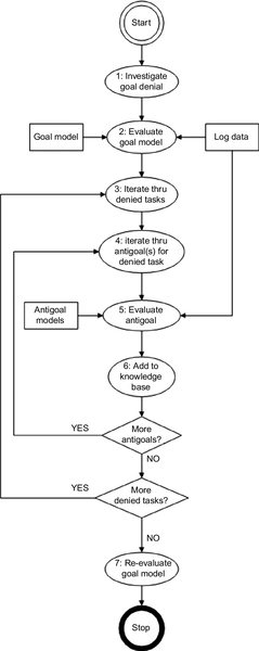
Step 1: The investigation starts when an alarm is raised or when the system administrator observes the failure of the monitored service, which is the denial of a goal g.
Step 2: On the basis of the knowledge base, which consists of all goal models and all observations (filtered log data and visual observation of the failure of the monitored service), the framework constructs a Markov network, which in turn is applied to generate a probability distribution for all the Satisfied(node, timestep) predicates for all nodes in the goal tree rooted at the denied goal g and the nodes of all other trees connected to it. This probability distribution is used to indicate the satisfaction or denial of tasks and goals at every timestep in the observation period. More specifically, if the probability of satisfaction of a task ai at a timestep t is higher than a threshold value thrs, then we conclude that ai is satisfied at t—that is, Satisfied(ai, t). Typically the timestep t starts at 0, and thrs is chosen to be 0.5.
An example of the outcome of this step is as follows based on Figure 18.9:


Step 3: The outcome of the previous step is a ranked list of denied tasks/goals, where the first task represents the node that is most likely to be the cause of the failure. In step 3, the framework iterates through the denied list of tasks identified in step 2, and loads the antigoal models targeting each of the denied tasks.
Step 4: For each antigoal model selected in step 3, we generate the observation literals from the log data by applying the ground atom generation process described in Section 18.7.1.5. Note that a task may have zero, one, or multiple antigoal models targeting it. The goal model in Figure 18.9 contains task a2, which has no antigoal models targeting it, task a1, which has one antigoal (ag1) targeting it, and task a3, which has two antigoals (ag3 and ag5) targeting it.
Step 5: This step is similar to step 2, but instead of evaluating a goal model, the framework evaluates the antigoal model identified in step 4 using the log-data-based observation and determines wether the top antigoal is satisfied. This is done by constructing a Markov network based on the antigoal model relationships (see Section 18.8.1) and inferring the probability distribution for the Satisfied(antigoal, timestep) predicate for the nodes in the antigoal model. In particular, we are interested in the probability assigned to Satisfied(agj, t) where t represents the timestep at which agj is expected to finish. Using the example in Figure 18.9, we see ag1 takes 11 steps to complete execution, while ag3 takes seven steps. In this case, we are interested in Satisfied(ag1,11) and Satisfied(ag2,7).
Step 6: On the basis of the value of Satisfied(agj, t) identified in step 5, we distinguish the following two cases:
(a) If Satisfied(agj, t) ≥ thrs (typically thrs = 0.5), this indicates that agj is likely to have occurred and caused ai to be denied. In this case, we add this information (antigoal and its relationship with the denied task) to the knowledge base. This knowledge base enrichment is done at two levels: first, a new observation is added to indicate that antigoal agj has occurred, and second, a rule is added on the basis of the pattern in Equation 18.18.
(b) If Satisfied(agj, t) < thrs, this indicates that agj did not occur; thus we exclude it as a potential cause of failure for ai.
Before going to next step, the framework checks whether the denied task ai is targeted by any other antigoal models. If it is, it iterates through the list of other antigoals agj that are targeting ai by going back to step 4. Once all antigoals targeting a denied task ai have been evaluated, the framework checks whether there are more denied tasks, and if there are, it repeats step 2.
Step 7: On the basis of the new knowledge acquired from evaluating the antigoal models, the satisfaction of tasks based on the enriched knowledge base is reevaluated to produce a new ranking of the denied tasks. The fact that an attack is likely to have occurred targeting a specific task that has failed increases the chances that this task is actually denied because of the intrusion, leading to the overall system failure. This overall process helps improve the diagnosis, but also provides interpretation for the denial of tasks.
18.9 Experimental Evaluations
To evaluate the proposed framework, we conducted the following set of case studies. The first set aims at examining the diagnostic effectiveness of the framework, using the experimental setup described in Section 18.4.4, by detecting root causes of observed failures due to internal errors. The second set focuses on detecting root causes of observed failures due to external actions. Finally, the third set aims to evaluate the scalability and measure the performance of the framework using larger data sets.
18.9.1 Detecting Root Causes due to Internal Faults
The first case study consists of a set of scenarios conducted using the loan application service. These scenarios are conducted from the perspective of the system administrator, where a system failure is reported, and a root cause investigation is triggered.
The normal execution scenario for the system starts with the receipt of a loan application in the form of a Web service request. The loan applicant’s information is extracted and used to build another request, which is sent to a credit evaluation Web service as illustrated in Figure 18.3.
The four scenarios in this study include one success and three failure scenarios (see Table 18.2). Scenario 1 represents a successful execution of the loan application process. Tthe denial of task a7 does not represent a failure in the process execution, since goal g3 is OR-decomposed into a6 (extract credit history for existing clients) and a7 (calculate credit history for new clients), and the successful execution of either a6 or a7 is enough for g3’s successful occurrence (see Figure 18.3). The probability values (weights) of the ground atoms range from 0 (denied) to 1 (satisfied). During each loan evaluation, and before the reply is sent to the requesting application, a copy of the decision is stored in a local table (a4 (update loan table)). Scenario 2 represents a failure to update the loan table leading to failure of top goal g1. Next, as described in Section 18.7.2.3, we identify a4 as the root cause of the failure. Note that although a7 was denied ahead of task a4, it is not the root cause since it is an OR child of g3, and its sibling task a6 was satisfied. Similarly, for scenario 3, we identify task a6 as the root cause of the failure. Scenario 4 represents the failure to validate Web service requests for the loan application. Almost no events are observed in this scenario. Using the diagnosis logic described in Section 18.7.2.3, we identify task a1 (receive loan application Web service request) as the root cause of the observed failure.
18.9.2 Detecting Root Causes due to External Actions
In this case study, we consider failures of the loan application scenario due to externally induced errors. As in the case of failures due to internal actions, we consider that the logs have the same format and the results are presented to the administrator in the same way—that is, in the form of lists of goal or antigoal nodes that correspond to problems that may be responsible (i.e., causes) for the observed failure. Each node is associated with a probability as this is computed by the reasoning engine as discussed in previous sections.
The experiment is conducted from the perspective of the system administrator, where a system failure is reported and an investigation is triggered. This case study scenario consists in running an attack while executing the credit history service (see the goal model of the credit service in Figure 18.7). The antigoal ag1 is executed by probing the active ports on the targeted machine, and then the attacker attempts to log in but uses a very long username (16,000 characters), disrupting the service authentication process, and denying legitimate users from accessing the service. Traces of this attack can be obtained in the Windows Event Viewer.
The antigoal ag2 models an SQL injection attack that aims at dropping the table containing the credit scores. One way to implement such an attack is to send two subsequent legitimate credit history Web service requests that contain embedded malicious SQL code within a data value. For example, to implement this malicious scenario, we embed an SQL command to scan and list all the tables in the data value of the field ID as follows:
The system extracts the credential data value (e.g., ID) and uses it to query the database, thus inadvertently executing the malicious code. The scan is followed by a second Web Service request that contains a command to drop the Credit_History table:
Traces of the credit service sessions are found in the SQL Server audit log data and in the message broker (hosting the credit service). The first antigoal ag1 represents the attacker’s plan to deny access to the credit service by keeping busy the port used by that service. The second antigoal ag2 aims at injecting an SQL statement that destroys the credit history data.
18.9.2.1 Experiment enactment
In this section, we outline a case where there is an observed failure, and we seek the possible causes. In this particular scenario there is a goal model and an antigoal model, and we illustrate how in the first phase of the process a collection of goal model nodes are identified as possible causes, but when in the second phase we consider also the antigoal model, where we identify the satisfaction of an antigoal that “targets” a goal node, the probability of the goal node failing (and thus becoming the leading cause) increases when we reevaluate it. The case is enacted with respect to the goal and antigoal models depicted in Figure 18.7.
We run a sequence of credit service requests and in parallel we perform an SQL injection attack. The log database table contained 1690 log entries generated from all systems in our test environment.
The first step in the diagnosis process (Figure 18.10) is to use the filtered log data to generate the observation (ground atoms) in the form of Boolean literals representing the truth values of the node annotations in the goal (or antigoal) model during the time interval where the log data is collected. The Planfile1 model segment below represents the observation corresponding to one credit service execution session:
Planfile1: Pre(g1,1); Pre(a1,1); Occ(a1,2); Post(a1,3); Pre(a2,3); Occ(a2,4); Post(a2,5); Post(g2,5); ?Pre(a5,5); ?Occ(a5,6); ?Post(a5,7); Pre(a6,5); ?Occ(a6,6); ?Post(a6,7); ?Post(g2,7); ?Pre(a3,7); ?Occ(a3,8); ?Post(a3,9); ?Pre(a4,9); ?Occ(a4,10); ?Post(a4,11); ?Post(g1,11), !Satisfied(g1,11)
In the case where we do not find evidence for the occurrence of the events corresponding to execution of goals/antigoals/tasks (precondition, postcondition, etc.), we do not treat this as proof that these events did not occur, but we consider them as uncertain. We represent this uncertainty by adding a question mark before the corresponding ground atoms. In cases where there is evidence that an event did not occur, the corresponding ground atom is preceded by an exclamation mark.
By applying inference based on the observation in Planfile1 (step 2 in the flowchart in Figure 18.10), we obtain the following probabilities for the ground atoms using the Alchemy tool:

Using step 2 in the diagnostics flowchart (Figure 18.10), we deduce that a4, a5, a6, and a3 are in that order, the possible root causes of the failure of the top goal g1 (i.e., they have the lowest success probability, meaning they have high failure probability).
Using steps 3 and 4 in the diagnostics flowchart, we first generate the observation for antigoal ag1 (Planfile2), and then apply inference based on the antigoal model ag1 relationship and the generated observation.
Planfile2: Pre(ag1,1), ?Pre(t1,1), ?Occ(t1,2), ?Post(t1,3), ?Pre(t2,3), ?Occ(t2,4), ?Post(t2,5), ?Pre(t3,5), ?Occ( t3,6), ?Post(t3,7), ?Post(ag1,7)
In step 5, the outcome of the inference indicates that ag1 is denied (satisfaction probability is 0.0001). We iterate through step 3, and the next denied task a5 is targeted by antigoal ag2. The observation generated for antigoal ag2 is depicted in the Planfile3 snipet below:
Planfile3: Pre(ag2,1), Pre(t4,1), Occ(t4,2), Post(t4,3), Pre(t5,3), Occ(t5,4), Post(t5,5), Pre(t6,5), Occ( t6,6), Post(t6,7), Post(ag2,7)
The outcome of the inference indicates that ag2 is satisfied (satisfaction probability is 0.59). Using step 6, we add the result to the goal model knowledge base. In step 7, we reevaluate the goal-model-based knowledge base and generate a new diagnosis as follows:

The new diagnosis now ranks a3 as the most likely root cause of the failure of the top goal g1 (i.e., it has the lowest success probability), whereas in the previous phase a4 was the most likely one. Next, a5, a4, and a6 are also possible root causes, but are now less likely. This new diagnosis is an improvement over the first one generated in step 2 since it accurately indicates a3 as the most probable root cause. We know that this is correct since the SQL injection attack ag2 targeted and dropped the credit table.
18.9.3 Performance Evaluation
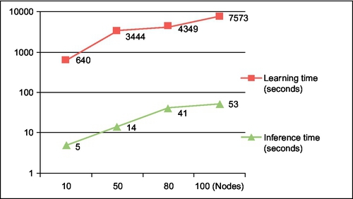
The third experiment is an evaluation of the processing performance of the framework. We used a set of extended goal models representing the loan application goal model to evaluate the performance of the framework when larger goal models are used. The four extended goal models contained 10, 50, 80, and 100 nodes, respectively. This experiment was conducted using Ubuntu Linux running on an Intel Pentium 2 Duo 2.2 GHz machine. From the experiments conducted, we observed that the matching and ground atom generation performance depends linearly on the size of the corresponding goal model and log data, and thus led us to believe that the process can easily scale for larger and more complex goal models. In particular, we are interested in measuring the impact of larger goal models on the learning and inference aspects of the framework.
Figure 18.11 illustrates that the number of ground atoms/clauses, which directly impacts the size of the resulting Markov model, is linearly proportional to the goal model size. Figure 18.12 illustrates that the running time for the off-line learning of the rule weights increases linearly with the size of the goal model. The learning time ranged from slightly over 10 min for a goal model with 10 nodes, to over 2 h for a model with 100 nodes. The inference time ranged from 5 s for a goal model with 10 nodes to 53 s for a model with 100 nodes. As the initial results indicate, this approach can be considered for applications with sizeable logs, entailing the use of small to medium-sized diagnostic models (approximately 100 nodes).

18.10 Conclusions
In this chapter, we have presented a root cause analysis framework that allows the identification of possible root causes of software failures that stem either from internal faults or from the actions of external agents. The framework uses goal models to associate system behavior with specific goals and actions that need be achieved in order for the system to deliver its intended functionality or meet its quality requirements. Similarly, the framework uses antigoal models to denote the negative impact the actions of an external agent may have on specific system goals. In this context, goal and antigoal models represent cause and effect relations and provide the means for denoting diagnostic knowledge for the system being examined. Goal and antigoal model nodes are annotated with pattern expressions. The purpose of the annotation expressions is twofold: first, to be used as queries in an information retrieval process that is based on LSI to reduce the volume of the logs to be considered for the satisfaction or denial of each node; and second, to be used as patterns for inferring the satisfaction of each node by satisfying the corresponding precondition, occurrence, and postcondition predicates attached to each node. Furthermore, the framework allows a transformation process to be applied so that a rule base can be generated from the specified goal and antigoal models.
The transformation process also allows the generation of observation facts from the log data obtained. The rule base and the fact base form a complete, for a particular session, diagnostic knowledge base. Finally, the framework uses a probabilistic reasoning engine that is based on the concept of Markov logic and MLNs. In this context, the use of a probabilistic reasoning engine is important as it allows inference to commence even in the presence of incomplete or partial log data, and ranking the root causes obtained by their probability or likelihood values.
The proposed framework provides some interesting new points for root cause analysis systems. First, it introduces the concept of log reduction to increase performance and is tractable. Second, it argues for the use of semantically rich and expressive models for denoting diagnostic knowledge such as goal and antigoal models. Finally, it argues that in real-life scenarios root cause analysis should be able to commence even with partial, incomplete, or missing log data information.
New areas and future directions that can be considered include new techniques for log reduction, new techniques for hypothesis selection, and tractable techniques for goal satisfaction and root cause analysis determination. More specifically, techniques that are based on complex event processing, information theory, or PLSI could serve as a starting point for log reduction. SAT solvers, such as Max-SAT and Weighted Max-SAT solvers, can also be considered as a starting point for generating and ranking root cause hypotheses on the basis of severity, occurrence probability, or system domain properties. Finally, the investigation of advanced fuzzy reasoning, probabilistic reasoning, and processing distribution techniques such as map-reduce algorithms may shed new light on the tractable identification of root causes for large-scale systems.