5.1.1 Definition of Displacement Power Factor

Displacement power factor (DPF) is the ratio of the active or real fundamental power P (measured in W or kW) to the fundamental apparent power S (measured in VA or kVA). The reactive power Q (measured in VAr or kVAr) supplied to inductive devices is the phasor difference between the real and apparent powers. The DPF is the cosine of the angle between these two quantities. It reflects how efficiently a facility uses electricity by comparing the amount of useful work that is extracted from the electrical apparent power supplied. Of course, there are many other measures of energy efficiency. The relationship between S, P, and Q is defined by the power triangle of Fig. 5.1.

$S^2=\sqrt{P^2+Q^2\text{.}}$

The DPF, determined from φ = tan^− 1(Q/P), measures the displacement angle between the fundamental components of the phase voltage and phase current:

$\mathrm{Displacement}\mathrm{power}\mathrm{factor}=\mathrm{D}\mathrm{P}\mathrm{F}=cos\mathrm{\phi }=P/S\text{.}$

The DPF varies between zero and one. A value of zero means that all power is supplied as reactive power and no useful work is accomplished. Unity DPF means that all of the power consumed by a facility goes to produce useful work, such as resistive heating and incandescent lighting.

Electric power systems usually experience lagging DPFs – based on the consumer notation of current – because a significant part consists of reactive devices that employ coils and requires reactive power to energize their magnetic circuits. Generally, motors that are operated at or near full nameplate ratings will have high DPFs (e.g., 0.90 to 0.95) whereas the same motor under no-load and/or light load conditions may exhibit a DPF in the range of 0.30. For example, motors in large hydraulic machines such as plastic molding machines mostly operate under lightly loaded conditions, contributing to an overall power factor of about 0.60.

The reactive power absorbed by electrical equipment such as transformers, electric motors, welding units, and static converters increases the currents of generators, transmission lines, utility transformers, switchgear, and cables. Electric utility companies must supply the entire apparent power demand. Because a customer only extracts useful work from the real power component, a high DPF is important. Therefore, in most power systems lagging (underexcited) DPFs (larger than 0.8) are acceptable, and leading (overexcited) power factors should be avoided because they may cause resonance conditions within the power system.

Inductive loads with low DPFs require the generators and transmission or distribution systems to supply reactive current with the associated power losses and increased voltage drops. If a shunt capacitor bank is connected across the load, its (capacitive) reactive current component I_C can cancel the load (inductive) reactive current component I_L. If the bank is sufficiently large (e.g., I_C = I_L), it will supply all reactive power, and there will be no reactive current flow entering the power system as is indicated in Fig. 5.2.

The DPF can be measured either by a direct-reading cosφ meter indicating an instantaneous value or by a recording VAr meter, which allows recording of current, voltage, and power factor over time. Readings taken over an extended period of time (e.g., seconds, minutes) provide a useful means of estimating an average value of power factor for an installation.

5.1.2 Total Power Factor (TPF) in the Presence of Harmonics

Equations 5-1 and 5-2 assume that system loads have linear voltage–current characteristics and harmonic distortions are not significant. Harmonic voltage and current distortions will change the expression for the total apparent power and the total power factor (TPF). Consider a voltage v(t) and a current i(t) expressed in terms of their rms harmonic components:

$v\left(t\right)=V_0+{\displaystyle \sum _{h=1}^{\infty }\sqrt{2}}{V}_{h}sin\left(h{\mathrm{\omega }}_{1}t+{\theta }_h^v\right)\text{,}$

$i\left(t\right)=I_0+{\displaystyle \sum _{h=1}^{\infty }\sqrt{2}}{I}_{h}sin\left(h{\mathrm{\omega }}_{1}t+{\theta }_h^i\right)\text{.}$

The active (real, average) and reactive powers are given by

$P_{\mathrm{total}}=V_o{I}_o+{\displaystyle \sum _{h=1}^{\infty }{V}_h{I}_{h}cos\left({\theta }_h^v-{\theta }_h^i\right)}\text{,}$

$Q_{\mathrm{total}}={\displaystyle \sum _{h=1}^{\infty }{V}_h{I}_{h}sin\left({\theta }_h^v-{\theta }_h^i\right)}\text{,}$

and the apparent (voltampere) power is

$S_{\mathrm{total}}=\sqrt{\left({\displaystyle \sum _{h=0}^{\infty }{I}_h^2)}\right({\displaystyle \sum _{h=0}^{\infty }{V}_h^2)\text{.}}}$

Therefore, for nonsinusoidal cases, Eq. 5-1 does not hold and must be replaced by

$D=\sqrt{S_{\mathrm{total}}^2-P_{\mathrm{total}}^2-Q_{\mathrm{total}}^2}\text{,}$

where D is called the distortion power.

According to Eq. 5–5, the TPF is lower than the DPF (Eq. 5–2) in the presence of harmonic distortion of nonlinear devices such as solid-state or switched power supplies, variable-speed AC drives, and DC drives. Harmonic distortion essentially converts a portion of the useful energy into high-frequency energy that is no longer useful to most devices and is ultimately lost as heat. In this way, harmonic distortion further reduces the power factor. In the presence of harmonics, the total power factor is defined as

$\mathrm{Total}\mathrm{power}\mathrm{factor}=\mathrm{T}\mathrm{P}\mathrm{F}=cos\theta =\frac{P_{\mathrm{total}}}{S_{\mathrm{total}}}\text{,}$

where P_total and S_total are defined in Eq. 5–4. Since capacitors only provide reactive power at the fundamental frequency, they cannot correct the power factor in the presence of harmonics. In fact, improper capacitor sizing and placements can decrease the power factor by generating harmonic resonances, which increase the harmonic content of system voltage and current. DPF = cosφ (with φ = tan^− 1(Q/P)) is always greater than TPF = cosθ (with θ = cos^− 1(P_totaL/S_total)) when harmonics are present. The DPF is still very important to most industrial customers because utility billing with respect to power factor is almost universally based on the displacement power factor.

5.1.2.1 Application Example 5.1: Computation of Displacement Power Factor (DPF) and Total Power Factor (TPF)

Strong power systems have very small system impedances (e.g., R_syst = 0.001 Ω, and X_syst = 0.005 Ω) whereas weak power systems have fairly large system impedances (e.g., R_syst = 0.1 Ω, and X_syst = 0.5 Ω). Power quality problems are mostly associated with weak systems. Unfortunately, distributed generation (DG) inherently leads to weak systems because the source impedances of small generators are large, that is, they cannot supply a large current (ideally infinitely large) during transient operation. This application example studies the power-factor correction for a relatively weak power system where the difference between the DPF and the TPF is large due to the relatively large amplitudes of voltage and current harmonics.

a) Perform a PSpice analysis for the circuit of Fig. E5.1.1, where a three-phase thyristor rectifier – fed by a Y/Y transformer with turns ratio (N_p/N_s = 1) – via a filter (e.g., capacitor C_f) serves a load (R_load). You may assume R_syst = 0.05 Ω, X_syst = 0.1 Ω, f = 60 Hz, v_AN(t) = $\sqrt{2}$·346 V cosωt, v_BN(t) = $\sqrt{2}$·346 V cos(ωt – 120°), and v_CN (t) = $\sqrt{2}$·346 V cos(ωt – 240°). Thyristors T₁ to T₆ can be modeled by metal-oxide-semiconductor field-effect transistors (MOSFETs) in series with diodes, C_f = 500 μF, R_load = 10 Ω, and a firing angle of α = 0°. Plot one period of the voltage and current after steady state has been reached as requested in parts b and c.

b) Plot and subject the line-to-neutral voltage v_an(t) to a Fourier analysis.

c) Plot and subject the phase current i_a(t) to a Fourier analysis.

d) Repeat parts a to c for α = 10°, 20°, 30°, 40°, 50°, 60°, 70°, and 80°.

e) Calculate the DPF and the TPF based on the phase shifts of the fundamental and harmonics between v_an(t) and i_a(t) for all firing angles and plot the DPF and TPF as a function of the firing angle α.

f) Determine the capacitance (per phase) C_bank of the power-factor correction capacitor bank such that the DPF as seen by the power system is for α = 60° about equal to DPF = 0.90 lagging.

g) Explain why the TPF cannot be significantly increased by the capacitor bank. Would the replacement of the capacitor bank by a three-phase tuned (R_fbank, L_fbank, and C_fbank) filter be a solution to this problem?

Solution to Application Example 5.1

a) The PSpice code for the circuit of Fig. E5.1.1 is given in Table E5.1.1

b) For parts b to d, Figs. E5.1.2 to E5.1.4 show the line to neutral (phase) voltage v_an(t) and the phase current i_a(t) for α = 10°, 40°, and 80°, respectively. Table E5.1.2 lists the Fourier coefficients (magnitude and phase angles) for the phase voltage v_an(t) and phase current i_a(t) as a function of α.

Table E5.1.2

Fourier components of v_an(t) and i_a(t) for the firing angles α = 10°, 40 °, and 80 °

α = 10°	vanh [V]	∠vanh [°]	iah [A]	∠ iah[°]
h = 1	482.5	− 144.6	75.9	− 170.5
h = 5	30.52	− 47.91	60.76	47.8
h = 7	33.62	− 153.5	47.93	− 112.4
α = 40°	vanh [V]	$\angle$ vanh [°]	iah [A]	$\angle$ iah[°]
h = 1	483.8	− 144.1	49.86	163.1
h = 5	21.92	179.9	43.64	− 84.45
h = 7	26.63	− 32.15	37.98	61.99
α = 80°	vanh [V]	$\angle$ vanh [°]	iah [A]	$\angle$ iah[°]
h = 1	488.8	− 144.0	4.666	129.8
h = 5	2.274	12.87	4.537	109
h = 7	3.097	94.55	4.403	− 171.4

c) Table E5.1.3 gives a summary of the DPF and TPF and their ratio (TPF/DPF) as a function of the firing angle α, Fig. E5.1.5 shows the DPF and TPF as a function of α, and Figure E5.1.5 shows that the DPF as a function of the firing angle α obeys the relation cosφ = 0.955 cosα [14]. Figure E5.1.6 illustrates the ratio (TPF/DPF) as a function of the firing angle α.

d) By introducing the capacitor bank into the above PSpice program and performing a series of runs for capacitor bank capacitance values C_bank from 400 to 10 μF one finds that for C_bank = 115 μF a DPF value of 0.9178 lagging is obtained. Figure E5.1.7 illustrates the voltage v_an(t) and i_a(t) for this case. These wave shapes demonstrate that a resonance condition exists: the capacitor bank with the capacitance C_bank = 115 μF is able to increase the DPF but is unable to reduce the harmonic components of voltages and currents, indeed the harmonic components are increased due to the resonance condition.

e) As mentioned above the DPF can be increased but the harmonics are increased due to resonance. The solution to this power factor correction problem is the replacement of the capacitor bank (with the capacitance value C_bank) by a passive filter Z_f consisting of a series connection of an inductor L_f and a capacitor C_f, which can be tuned to an appropriate frequency.

5.1.3 Benefits of Power-Factor Correction

Improving a facility’s power factor (either DPF or TPF) not only reduces utility power factor surcharges, but it can also provide lower power consumption and offer other advantages such as reduced demand charges, increased load-carrying capabilities in existing lines and circuits, improved voltage profiles, and reduced power system losses. The overall results are lower costs to consumers and the utility alike, as summarized below:

• Increased Load-Carrying Capabilities in Existing Circuits. Installing a capacitor bank at the end of a feeder (near inductive loads) improves the power factor and reduces the current carried by the feeder. This may allow the circuit to carry additional loads and save costs for upgrading the network when extra capacity is required. In addition, the lower current flow reduces resistive losses in the circuit.

• Improved Voltage Profile. A lower power factor requires a higher current flow for a given load. As the line current increases, the voltage drop in the conductor increases, which may result in a lower voltage at the load. With an improved power factor, the voltage drop in the conductor is reduced.

• Reduced Power-System Losses. In industrial distribution systems, active losses vary from 2.5 to 7.5% of the total load measured in kWh, depending on hours of full-load and no-load plant operation, wire size, and length of the feeders. Although the financial return from conductor loss reduction alone is seldom sufficient to justify the installation of capacitors, it is an attractive additional benefit, especially in older plants with long feeders. Conductor losses are proportional to the current squared, whereas the current is reduced in direct proportion to the power-factor improvement; therefore, losses are inversely proportional to the square of the power factor.

• Release of Power-System Capacity. When capacitor banks are in operation, they furnish magnetizing current for electromagnetic devices (e.g., motors, transformers), thus reducing the current demand from the power plant. Less current means less apparent power, or less loading of transformers and feeders. This means capacitors can be used to reduce system overloading and permit additional load to be added to existing facilities. Release of system capacity by power-factor improvement and especially with capacitors has become an important practice for distribution engineers.

• Reducing Electricity Bills. To encourage more efficient use of electricity and to allow the utility to recoup the higher costs of providing service to customers with low power factor demanding a high amount of current, many utilities require that the consumers improve the power factors of their installations. This may be in the form of power-factor penalty (e.g., adjusted demand charges or an overall adjustment to the bill) or a rate structure (e.g., the demand charges or power rates are based on current or apparent power). Power-factor penalties are usually imposed on larger commercial and industrial customers when their power factors fall below a certain value (e.g., 0.90 or 0.95). Customers with current or apparent power-based demand charges in effect pay more whenever their power factor is less than about unity. More and more utilities are introducing power-factor penalties (or apparent power-based demand charges) into their rate structures, in part to comply with provisions of the Clean Air Act and deregulation, and to some extent in response to growing competition in a newly deregulated power market. Without these surcharges there would be no motivation for consumers to install power-factor correction facilities. Against the financial advantages of reduced billing, the consumer must balance the cost of purchasing, installing, and maintaining the power-factor-improvement capacitors. The overall result of enforcing incentives is lower costs to consumers and the utility companies. A high power factor avoids penalties imposed by utilities and makes better use of the available capacity of a power system.

Therefore, power-factor correction capacitors are usually installed in power systems to improve the efficiency at which electrical energy is delivered and to avoid penalties imposed by utilities, making better use of the available capacity of a power system.

5.3.1 Application Example 5.2: Design of a Tuned Harmonic Filter

A harmonic LC filter (consisting of a capacitor C in series with an inductor L) is to be designed in parallel to a power-factor correction (PFC) capacitor C_bank to improve the power quality (as recommended by IEEE-519 [8]) and to improve the DPF from cosφ_load = 0.42 lagging to 0.97 lagging (consumer notation). Data obtained from a harmonic analyzer at 30% loading are 6.35 kV/phase, 618 kW/phase, DPF = 0.42 lagging, THD _i = 30.47%, fundamental frequency f = 50 Hz, and fifth harmonic (250 Hz) current I₅ = 39.25 A.

Solution to Application Example 5.2

Figure E5.2.1 shows the per-phase equivalent circuit of the nonlinear load generating 5th harmonic current whereby the tuned series LC filter and the DPF correcting capacitor bank are not connected. Note that cosφ_load = 0.42 lagging, φ_load = cos^− 1(0.42) = − 1.13735 rad ≡ − 66.1673°. Figure E5.5.2 illustrates the phasor diagram for real (P), reactive (Q), and complex ($\tilde{S}$) powers. At 30% loading the data are $\left|{\tilde{V}}_{\mathit{phase}}\right|=$ 6.35 kV per phase, P_{load_30%} = 618 kW per phase, DPF = 0.42 lagging, THD_i = 30.47%, f = 50 Hz, $\left|{\tilde{I}}_5\right|=I_5=$ 39.5A. Figure E5.2.3 illustrates the per-phase circuit when the tuned LC filter and the DPF cosφ_load correcting capacitor bank are present.

• Calculation of the required reactive power Q_required for improving DPF to the desired value: cosφ_compensated = 0.97lagging, φ_compensated = cos^− 1(0.97) = − 0.245566 rad ≡ − 14.0703°. P = P_{load_30%} = P_{compensated_30%} = constant = 618 kW/phase. From the phasor diagram of Figure E5.2.2 one obtains Q_{load_30%} = P_{load_30%} ∙ tanφ_load < 0, Q_{compensated_30%} = P_{load_30%} ∙ tanφ_compensated < 0, Q_{required_30%} = P_{load_30%} (tanφ_{compensated_30%} - tanφ_load) > 0, Q_{required_30%} = 618 kW [tan(− 14.0703°) - tan(− 65.1673°)] > 0,

$Q_{\mathit{required}\_30\%}=618\mathrm{kW}\left[-0.250624-\left(-2.16077\right)\right]=1180.47\mathrm{kVAr}/\mathrm{phase}>0\text{.}$

• According to IEEE-519 [8], THD_i should drop from 30.47% to 4.0%. We employ about 30% of the required Q_required for filtering (tuned) and the remaining for (untuned) displacement power factor compensation (DPFC). Select filter capacitance to supply 30% of Q_{required_30%}:

$Q_{\mathit{filter}\_30\%}=0.3Q_{\mathit{required}\_30\%}=0.3·1180.47\mathrm{kVAr}/\mathrm{phase}=354.141\mathrm{kVAr}/\mathrm{phase}>0\text{.}$

• Assuming Y-connected (filter) capacitor banks one obtains with Q = VI = V²/X_C or X_C = V²/Q.

From this follows for the fundamental (1) reactance and the 5th harmonic (5) reactance $X_C^{\left(1\right)}=\frac{{\left(6.35k\right)}^2{V}^2}{354.14\mathit{kVAr}}=113.86\mathrm{\Omega }/\mathrm{phase}=1/\left(\mathrm{\omega }\mathrm{C}\right)\text{,}$ or $C=\frac{1}{2\mathrm{\pi }\cdot 50\cdot 113.86}=27.9571\mathit{\mu }\mathrm{F}\text{.}$$X_C^{\left(5\right)}=X_C^{\left(1\right)}/5=\left(113.86/5\right)\mathrm{\Omega }/\mathrm{phase}=22.772\mathrm{\Omega }/\mathrm{phase}\text{.}$

The tuned filter requires: $X_L^{\left(5\right)}=X_C^{\left(5\right)}=$ 22.772 Ω/phase.

$X_L^{\left(1\right)}=X_L^{\left(5\right)}/5=$ (22.772/5) = 4.5544 Ω/phase or $L=\frac{X_L^{\left(5\right)}}{2\pi \cdot 50\cdot 5}=\frac{22.772}{2\pi \cdot 50\cdot 5}=$ 14.4975 mH/phase.

Figure E5.2.4 shows the phasor diagram for current and voltages where the magnitude of voltage ${\tilde{V}}_{\mathit{L}}^{\left(1\right)}$ is very small as compared with ${\tilde{V}}_{\mathit{C}}^{\left(1\right)}$ and ${\tilde{V}}_{\mathit{phase}}={\tilde{V}}_{\mathit{phase}}^{\left(1\right)}$.

For $X_C^{\left(1\right)}>>X_{{}_L}^{\left(1\right)}$ or $\left|{\tilde{V}}_C^{\left(1\right)}\right|>>\left|{\tilde{V}}_L^{\left(1\right)}\right|$ or $\left|{\tilde{V}}_C^{\left(1\right)}\right|\approx \left|{\tilde{V}}_{\mathit{phase}}\right|$, one obtains $\left|{\tilde{I}}_C^{\left(1\right)}\right|\approx \left|{\tilde{V}}_{\mathit{phase}}\right|/X_{{}_C}^{\left(1\right)}=$ 6.35 kV/113.86 Ω = 55.77A = |Ĩ_L⁽¹⁾|, and $\left|{\tilde{I}}_C^{\left(5\right)}\right|=39.25\mathrm{A}=\left|{\tilde{I}}_L^{\left(5\right)}\right|$

Without tuned LC filter:

THD_i = 0.3047 = $\left|{\tilde{I}}_C^{\left(5\right)}\right|/\left|{\tilde{I}}_{\mathit{phase}}\right|$ and $\left|{\tilde{I}}_{\mathit{phase}}\right|=618\mathit{kW}/6.35\mathit{kV}\cdot 0.42=$ 231.7A, thus $\left|{\tilde{I}}_C^{\left(1\right)}\right|=$ 0.3047. 231.7A = 70.61A.

With tuned LC filter:

THD_i = 0 = $\left|{\tilde{I}}_C^{\left(5\right)}\right|/\left|{\tilde{I}}_{\mathit{phase}}\right|$ and $\left|{\tilde{I}}_{\mathit{phase}}\right|=618\mathit{kW}/6.35\mathit{kV}\cdot 0.97=100.3\mathrm{A}$, thus $\left|{\tilde{I}}_C^{\left(5\right)}\right|=0\cdot 100.3\mathrm{A}=0\mathrm{A}$, that is no harmonic current enters the supply system. Tuned filters have a resistive component and cannot be exactly tuned, because of temperature and manufacturing tolerances.

Although the fundamental and the fifth harmonic are not necessarily in phase, we assume the worst-case condition where both signals are in phase.

• Reactive power rating of inductor L of LC filter is with

$\left|{\tilde{V}}_L\right|=\left|{\tilde{V}}_L^{\left(1\right)}\right|+\left|{\tilde{V}}_L^{\left(5\right)}\right|=\left|{\tilde{I}}_L^{\left(1\right)}\right|X_L^{\left(1\right)}+\left|{\tilde{I}}_L^{\left(5\right)}\right|X_L^{\left(5\right)}=55.77\cdot 4.5544+39.25\cdot 22.772=1.1478\mathrm{kV}\text{,}$

$Q_{\mathit{rating}}^{\mathit{inductor}}=\left|{\tilde{V}}_L\right|I_{rms}=1.1478\mathrm{kV}\cdot 39.25\mathrm{A}=45.05\mathrm{kVAr}$

• Reactive power rating of capacitor C of LC filter is with

$\left|{\tilde{V}}_C\right|=\left|{\tilde{V}}_C^{\left(1\right)}\right|+\left|{\tilde{V}}_C^{\left(5\right)}\right|=\left|{\tilde{I}}_C^{\left(1\right)}\right|X_C^{\left(1\right)}+\left|{\tilde{I}}_C^{\left(5\right)}\right|X_C^{\left(5\right)}=55.77\cdot 113.86+39.25\cdot 22.772=7.24377\mathrm{kV}\text{,}$

$Q_{\mathit{rating}}^{\mathit{capacitor}}=\left|{\tilde{V}}_C\right|I_{rms}=7.24377\mathrm{kV}\cdot 39.25\mathrm{A}=284.32\mathrm{kVAr}\text{.}$

• Current rating of capacitor bank C_bank at f = 50 Hz is $I_C^{\left(1\right)}=V_{\mathit{phase}}/X_C^{\left(1\right)}=6.35\mathrm{kV}/113.86\mathrm{\Omega }=55.77\mathrm{A}$, $\left|{\tilde{I}}_C^{\left(5\right)}\right|=$ 39.25A. Select based on Pythagorean theorem I_rms = 68A, resulting in $Q_{\mathit{rating}\_\mathit{final}}^{\mathit{inductor}}=\left|{\tilde{V}}_L\right|I_{rms}=1.1478\mathrm{kV}\cdot 68\mathrm{A}=78.05\mathrm{kVAr}$, and $Q_{\mathit{rating}\_\mathit{final}}^{\mathit{capacitor}}=\left|{\tilde{V}}_C\right|I_{rms}=7.24377\mathrm{kV}\cdot 68\mathrm{A}=492.58\mathrm{kVAr}$.

5.4.1 Transients Associated with Capacitor Switching

Transients associated with capacitor switching are generally not a problem for utility equipment. However, they could cause a number of problems for the customers, including

• voltage increases (overvoltages due to capacitor switching),

• transients can be magnified in a customer facility (e.g., if the customer has low-voltage, power-factor correction capacitors) resulting in equipment damage or failure (due to excessive overvoltages),

• nuisance tripping or shutdown (due to DC bus overvoltage) of adjustable-speed drives or other process equipment, even if the customer circuit does not employ any capacitors,

• computer network problems, and

• telephone and communication interference.

Because capacitor voltage cannot change instantaneously, energizing a capacitor bank results in an immediate drop in system voltage toward zero, followed by a fast voltage recovery (overshoot), and finally an oscillating transient voltage superimposed with the fundamental waveform (Fig. 5.3). The peak-voltage magnitude (up to 2 pu with transient frequencies of 300–1000 Hz) depends on the instantaneous system voltage at the moment of capacitor connection.

Voltage increase occurs when the transient oscillation – caused by the energization of a capacitor bank – excites a series resonance formed by the leakage inductances of a low-voltage system. The result is an overvoltage at the low-voltage bus. The worst voltage transients occur when the following conditions are met:

• The size of the switched capacitor bank is significantly larger (> 10) than the low-voltage power-factor correction bank;

• The source frequency is close to the series-resonant frequency formed by the step-down transformer and the power-factor correction-capacitor bank; and

• There is relatively small damping provided by the low-voltage load (e.g., for typical industrial plant configuration or primarily motor load with high efficiency).
Solutions to the voltage increase usually involve:

• Detune the circuit by changing capacitor bank sizes;

• Switch large banks in more than one section of the system;

• Use an overvoltage control method. For example, use switching devices that do not prestrike or restrike, employ synchronous switching of capacitors, and install high-energy metal-oxide surge arrestors to limit overvoltage and protect critical equipment;

• Apply surge arresters at locations where overvoltages occur;

• Convert low-voltage power-factor correction banks into harmonic filters (e.g., detune the circuit);

• Use properly designed and tuned filters instead of capacitors;

• Install isolation or dedicated transformers or series reactors for areas of sensitive loads; and

• Rely on transient-voltage-surge suppressors.

5.4.2 Harmonic Resonances

Improper placement and sizing of capacitors could cause parallel and/or series resonances and tune the system to a frequency that is excited by a harmonic source [7]. In industrial power systems, capacitor banks are normally specified for PFC, filtering, or reactive-power compensation without regard to resonances and other harmonic concerns. High overvoltages could result if the system is tuned to one harmonic only that is being supplied by a nonlinear load or saturated electromagnetic device such as a transformer (e.g., second, third, fourth, and fifth harmonics result from transformer inrush currents). Moreover, the capacitive reactance is inversely proportional to frequency; therefore, harmonic currents may overload capacitors beyond their limits. Thus, capacitor banks themselves may be affected by resonance, and may fail prematurely. This may even lead to plant or feeder shutdowns.

Resonance is a condition where the capacitive reactance of a system offsets its inductive reactance, leaving the small resistive elements in the network as the only means of limiting resonant currents. Depending on how the reactive elements are arranged throughout the system, the resonance can be of a series or a parallel type. The frequency at which this offsetting effect takes place is called the resonant frequency of the system.

5.4.3 Application Example 5.3: Harmonic Resonance in a Distorted Industrial Power System with Nonlinear Loads

Figure E5.3.1a shows a simplified industrial power system (R_sys = 0.06 Ω, L_sys = 0.11 mH) with a power-factor correction capacitor (C_pf = 1300 μF). Industrial loads may have nonlinear (v–i) characteristics that can be approximately modeled as (constant) decoupled harmonic current sources. The utility voltages of industrial distribution systems are often distorted due to the neighboring loads and can be approximately modeled as decoupled harmonic voltage sources (as shown in the equivalent circuit of Fig. E5.3.1b):

$v_{\mathrm{s}\mathrm{y}\mathrm{s}}\left(t\right)={\displaystyle \sum _{h=1}^{\infty }{v}_{\mathrm{s}\mathrm{y}\mathrm{s},h}}\left(t\right)={\displaystyle \sum _{h=1}^{\infty }\sqrt{2}}{V}_{s\mathrm{y}\mathrm{s},h}sin\left(h{\mathrm{\omega }}_{1}t+{\theta }_{\mathrm{s}\mathrm{y}\mathrm{s},h}^v\right)\text{,}$

$i_{NL}\left(t\right)={\displaystyle \sum _{h=1}^{\infty }{i}_{NL,h}}\left(t\right)={\displaystyle \sum _{h=1}^{\infty }\sqrt{2}}{I}_{NL,h}sin\left(h{\mathrm{\omega }}_{1}t+{\theta }_{NL,h}^i\right)\text{.}$

Fourier analyses of measured voltage and current waveforms of the utility system and the nonlinear loads can be used to estimate the values of V_sys,h, θ_sys,h^v, I_NL,h, and θ_NL,hⁱ. This is a practical approach because most industrial loads consist of a number of in-house nonlinear loads, and their harmonic models are not usually available.

For this example, assume

$v_{\mathrm{s}\mathrm{y}\mathrm{s}}\left(t\right)=\sqrt{2}\left(110\right)sin\left({\mathrm{\omega }}_{1}t\right)+\sqrt{2}\left(3\right)sin\left(5{\mathrm{\omega }}_{1}t\right)+\sqrt{2}\left(2\right)sin\left(7{\mathrm{\omega }}_{1}t\right)\left[\mathrm{V}\right]\text{,}$

$i_{NL}\left(t\right)=\sqrt{2}\left(1.0\right)sin\left({\mathrm{\omega }}_{1}t\right)+\sqrt{2}\left(0.3\right)sin\left(5{\mathrm{\omega }}_{1}t\right)+\sqrt{2}\left(0.2\right)sin\left(7{\mathrm{\omega }}_{1}t\right)\left[\mathrm{A}\right]\text{.}$

Compute frequencies of the series and parallel resonances and the harmonic currents injected into the capacitor, and plot its frequency response.

Solution to Application Example 5.3

i) To observe the effect of the nonlinear load, the harmonic voltage source (representing the distorted utility voltage) is assumed to be short-circuited. The harmonic current injected into the capacitor due to the nonlinear load is

${\tilde{I}}_{C,h}^{\mathrm{due}NL}=\frac{Z_{sys,h}}{Z_{sys,h}+Z_{C,h}}{\tilde{I}}_{NL,h}\text{.}$

A parallel resonance occurs when the denominator approaches zero. The frequency of the parallel resonance is

$f_{\mathrm{parallel}}=\frac{1}{2\pi \sqrt{L_{sys}C}}=\frac{1}{2\pi \sqrt{0.11m\cdot 1300\mathit{\mu }}}\approx 420\mathrm{Hz}\text{.}$

This condition will result in a large harmonic current being injected into the capacitor bank. The magnitude of the injected harmonic current can be several times the rated capacitor current, and may result in extensive harmonic voltages across the capacitor. Therefore, parallel resonance may result in the destruction of the capacitor due to overvoltage or over-current conditions.

ii) To investigate the effect of the distorted utility voltage on the capacitor, the harmonic current source (approximating the nonlinear load) is assumed to be ideal, that is, its impedance approaches infinity and behaves like an open circuit. The harmonic current injected into the capacitor due to the distorted utility source is

${\tilde{I}}_{C,h}^{\mathrm{due}sys}=\frac{1}{Z_{sys,h}+Z_{C,h}}{\tilde{V}}_{sys,h}\text{.}$

A series resonance occurs when the denominator approaches zero. Therefore, for this system the frequencies of the series and parallel resonances are identical:

$f_{\mathrm{series}}=f_{\mathrm{parallel}}=\frac{1}{2\pi \sqrt{L_{sys}C}}\approx 420\mathrm{Hz}\text{.}$

The harmonic current injection into the power capacitor will be increased if the utility voltage contains harmonic components near resonance frequencies.

iii) The total harmonic current injected into the power capacitor is

$\begin{array}{c}{\tilde{I}}_{C,h}={\tilde{I}}_{C,h}^{\mathrm{due}NL}+{\tilde{I}}_{C,h}^{\mathrm{due}sys}=\frac{Z_{sys,h}}{Z_{sys,h}+Z_{C,h}}{\tilde{I}}_{NL,h}\\ +\frac{1}{Z_{sys,h}+Z_{C,h}}{\tilde{V}}_{sys,h}\text{.}\end{array}$

Therefore, the 5th harmonic component of the injected current into the capacitor is

$\begin{array}{c}{\tilde{I}}_{C,5}={\tilde{I}}_{C,5}^{\mathrm{due}NL}+{\tilde{I}}_{C,5}^{\mathrm{due}sys},\\ {\tilde{I}}_{C,5}^{\mathrm{due}NL}=\frac{Z_{sys,5}}{Z_{sys,5}+Z_{C,5}}{\tilde{I}}_{NL,5},\\ =\frac{\left[0.06+j5\left(2\pi \cdot 60\cdot 0.11\cdot {10}^{-3}\right)\right]{\tilde{I}}_{NL,5}}{\left[0.06+j5\left(2\pi \cdot 60\cdot 0.11\cdot {10}^{-3}\right)]-[j/5\left(2\pi \cdot 60\cdot 1300\cdot {10}^{-6}\right)\right]},\\ =\frac{0.06+j0.2074}{0.06+j0.2074-j0.408}{\tilde{I}}_{NL,5},\\ =\frac{0.06+j0.2074}{0.06-j0.2}{\tilde{I}}_{NL,5}=\frac{0.2159\angle 73.87°}{0.2\angle -73.3°}{\tilde{I}}_{NL,5},\\ =\left(1.08\angle 147.17°\right){\tilde{I}}_{NL,5},\\ =1.08\angle 147.17°)\left(\sqrt{2}\left(0.3\right)\angle 0°\right)\mathrm{A},\\ =\sqrt{2}\left(0.324\right)\angle 147.17°\mathrm{A}\text{.}\end{array}$

$\begin{array}{c}{\tilde{\mathrm{I}}}_{C,5}^{\mathrm{due}sys}=\frac{1}{X_{sys,5}+Z_{C,5}}{\tilde{V}}_{sys,5}=\frac{1}{0.2\angle -73.3°}{\tilde{V}}_{sys,5},\\ =\left(5\angle 73.3°\right){\tilde{V}}_{sys,5}=\left(5\angle 73.3°\right)\left(\sqrt{2}\left(3\right)\angle 0°\right)\mathrm{A},\\ =\sqrt{2}\left(15\right)\angle 73.3°\mathrm{A},\\ \Rightarrow \Rightarrow {\tilde{I}}_{C,5}={\tilde{I}}_{C,5}^{\mathrm{due}NL}+{\tilde{I}}_{C,5}^{\mathrm{due}sys},\\ =\left(\sqrt{2}\left(0.324\right)\angle 147.17°\right)+(\sqrt{2}\left(15\right)\angle 73.3°\mathrm{A},\\ =\sqrt{2}\left(4.04+j14.54\right)=\sqrt{2}\left(15.1\right)\angle 74.47°\mathrm{A}\text{.}\end{array}$

The 7th harmonic component of the injected current into the power capacitor is

$\begin{array}{c}{\tilde{I}}_{C,7}={\tilde{I}}_{C,7}^{\mathrm{due}NL}+{\tilde{I}}_{C,7}^{\mathrm{due}sys},\\ {\tilde{I}}_{C,7}^{\mathrm{due}NL}=\frac{Z_{sys,7}}{Z_{sys,7}+Z_{C,7}}{\tilde{I}}_{NL,7},\\ =\frac{\left[0.06+j7\left(2\pi \cdot 60\cdot 0.11\cdot {10}^{-3}\right)\right]{\tilde{I}}_{NL,7}}{0.06+j7\left(2\pi \cdot 60\cdot 0.11\cdot {10}^{-3}\right)-j/7\left(2\pi \cdot 60\cdot 1300\cdot {10}^{-6}\right)},\\ =\frac{0.06+j7\cdot 0.04147}{0.06+j7\cdot 0.04141-j2.040/7}{\tilde{I}}_{NL,7},\\ =\frac{0.06+j0.29029}{0.06-j0.0011}{\tilde{I}}_{NL,7}=\frac{0.2964\angle 78.32°}{0.06\angle -1.05°}{\tilde{I}}_{NL,7},\\ =\left(4.964\angle 79.37°\right){\tilde{I}}_{NL,7},\\ =\left(4.964\angle 79.37°\right)\left(\sqrt{2}\left(0.2\right)\angle 0°\right)\mathrm{A},\\ =\sqrt{2}\left(0.993\right)\angle 79.39°\mathrm{A}.\\ {\tilde{I}}_{C,7}^{\mathrm{due}sys}=\frac{1}{Z_{sys,7}+Z_{C,7}}{\tilde{V}}_{sys,7}=\frac{1}{0.06\angle -1.05°}{\tilde{V}}_{sys,7},\\ =\left(16.7\angle 1.05°\right){\tilde{V}}_{sys,7},\\ =\left(16.7\angle 1.05°\right)\left(\sqrt{5}\left(2\right)\angle 0°\right)\mathrm{A},\\ =\sqrt{2}\left(33.4\right)\angle 1.05°\mathrm{A},\\ \Rightarrow \Rightarrow {\tilde{I}}_{C,7}={\tilde{I}}_{C,7}^{\mathrm{due}NL}+{\tilde{I}}_{C,7}^{\mathit{due}sys},\\ =\left(\sqrt{2}\left(0.993\right)\angle 79.37°\right)+\left(\sqrt{2}\left(33.4\right)\angle 1.05°\right)\mathrm{A},\\ =\sqrt{2}\left(33.58+1.59\right)\mathrm{A},\\ =\sqrt{2}\left(33.62\right)\angle 2.7°\mathrm{A}\text{.}\end{array}$

iv) As expected, the 7th harmonic current of the nonlinear load and the distorted utility voltage are magnified (it is a relatively weak system; R_sys = 0.06 Ω and X_sys = 2π(60)(0.11 × 10^− 3) = 0.042 Ω) due to the parallel and series and resonances at f = 420 Hz.

v) The frequency responses of the capacitor current divided by the load harmonic current and divided by the utility harmonic voltage are shown in Fig. E5.3.2.

5.4.4 Application Example 5.4: Parallel Resonance Caused by Capacitors

The single-phase diagram and the equivalent circuit (neglecting resistances) are shown in Figs E5.4.1a, b. In Fig. E5.4.1a, the source has the ratio X/R = 10. Assume X/R = 4000 (losses 0.25 W/kVAr) and X/R = 5000 (losses 0.2 W/kVAr) for low-voltage and medium-voltage high-efficiency capacitors, respectively. The harmonic current source is a six-pulse converter injecting harmonic currents of the order [8]

$h=n\left(k+1\right)$

where n is an integer (typically from 1 to 4) and k is the number of pulses (e.g., equal to 6 for a six-pulse converter). Find the resonance frequency of this circuit. Plot the frequency response and current amplification at bus 1.

Solution to Application Example 5.4

The resonance frequency is with S_sc = MVA_sc and Q_cap = MVAr_cap

$h=\sqrt{\frac{MV{A}_{SC}}{MVA{r}_{\mathrm{cap}}}}$

This is a characteristic frequency of the six-pulse nonlinear load.

From $h=\sqrt{MV{A}_{sc}/MVA{r}_{\mathit{cap}}}$, with MVA_sc = 72.6 MVA per phase, MVAr_cap = 0.6 MVAr per phase follows $h=\sqrt{72.6/0.6}=11$.

Calculation of system inductance L_sys per phase:

S_sc = MVA_sc = V_ph∙ I_ph= $V_{\mathit{ph}}^2/\left[\sqrt{R_{sys}^2+{\left(\mathit{\omega }{L}_{sys}\right)}^2}\right]$, $R_{sys}=X_{sys}/10$, therefore S_sc= $V_{\mathit{ph}}^2/\left[\sqrt{{\left(\mathit{\omega }{L}_{sys}/10\right)}^2+{\left(\mathit{\omega }{L}_{sys}\right)}^2}\right]=V_{\mathit{ph}}^2/\left[\mathit{\omega }{L}_{sys}\sqrt{{\left(1/10\right)}^2+{\left(1\right)}^2}\right]$, with S_sc = (72.6 + 0.48)MVA = 73.08MVA, V_ph = 4.16 kV follows $73.08\cdot {10}^6=\left[{\left(4.16\right)}^2\cdot {10}^6\right]/\left[377\cdot L_{sys}\cdot 1.005\right]$ or L_sys = 0.625 mH, where ω = 2πf = 2π60 ≈ 377 rad/s.

Calculation of C of capacitor bank:

$Q=V_{\mathit{ph}}^2/\left[1/\mathit{\omega }C\right]$ or $C=0.6\cdot {10}^6/\left[377\cdot {\left(4.16\right)}^2\cdot {10}^6\right]=91.97\mathit{\mu }F$

Equivalent system impedance neglecting resistances:

$Z^h=\frac{\left(1/\mathit{jh}\mathit{\omega }\mathit{C}\right)jh\mathit{\omega }{L}_{sys}}{\left(1/j\mathit{\omega }C\right)+jh\mathit{\omega }{L}_{sys}}=\frac{0.625m/91.97\mathit{\mu }}{j\left[h\cdot 377\cdot 0.625m-1/\left(h\cdot 377\cdot 91.97\mathit{\mu }\right)\right]}\text{.}$

For h = 1,

$Z^{h=1}=\frac{6.796}{j\left[377\cdot 0.625m-1/\left(377\cdot 91.97\mathit{\mu }\right)\right]}=j0.2376\mathrm{\Omega }\text{.}$

For h = 13,

$Z^{h=13}=\frac{6.796}{j\left[13\cdot 377\cdot 0.625m-1/\left(13\cdot 377\cdot 91.97\mathit{\mu }\right)\right]}=-j8.048\mathrm{\Omega }\text{.}$

Figure E5.4.1c illustrates for h = 1 to 13 the $Z_{mag\_\mathit{without}\_\mathit{loss}}^h=\left|Z_{\mathit{without}\_\mathit{loss}}^h\right|$ = f (h) without resistive damping (loss), which is a plot of the equivalent system impedance magnitude as seen from bus 1. This plot is known as a frequency scan.

One determines the ratio $\left[\right(i_{C,h}/i_h)=h\mathrm{\omega }{L}_{sys}/(h\mathrm{\omega }{L}_{sys}-1/h\mathrm{\omega }C)]$, and correspondingly, $[(i_{sys,h}/i_h)=(-1/h\mathrm{\omega }C)/(h\mathrm{\omega }{L}_{sys}-1/h\mathrm{\omega }C)]$.

For h = 1,

$\begin{array}{c}\frac{i_{C,1}}{i_1}=\frac{377\cdot 0.625m}{377\cdot 0.625m-1/\left(377\cdot 91.97\cdot {10}^{-6}\right)}=-0.00824\mathrm{p}\mathrm{u},\\ \frac{i_{sys,1}}{i_1}=\frac{-28.84}{0.2356-28.84}=1.008\mathrm{p}\mathrm{u}\text{.}\end{array}$

For h = 13,

$\begin{array}{c}\frac{i_{C,13}}{i_{13}}=\frac{13\cdot 377\cdot 0.625m}{13\cdot 377\cdot 0.625m-1/\left(13\cdot 377\cdot 91.97\cdot {10}^{-6}\right)}=3.627\mathrm{p}\mathrm{u},\\ \frac{i_{sys,13}}{i_{13}}=\frac{-2.219}{3.063-2.219}=-2.629\mathrm{p}\mathrm{u}.\end{array}$

The absolute values of i_C,_h/i_h and i_{sys, h}/i_h for h = 1 to 13 are depicted in Figures E5.4.2a,b respectively, as a function of h without resistive damping (loss), which is the current amplification.

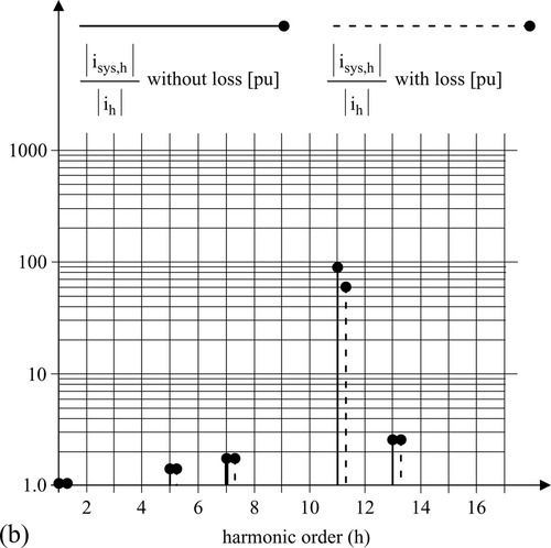
Taking the resistive components into account yields the following relations and values:

X_sys = 10R_sys or R_sys = ωL_sys/10 = (377.0.625 m)/10 = 0.02356 Ω. For low-voltage capacitors X_C/R_C = 4000 Ω or $R_C=X_C/4000=\left[1/\left(377\cdot 91.97\cdot {10}^{-6}\right)\right]/\left(4000\right)=0.00721\mathrm{\Omega }$

The impedances are: $\begin{array}{l}{Z}_{sys}^h=R_{sys}+jh\mathrm{\omega }{L}_{sys}\mathrm{and}{Z}_C^h=R_C+1/\mathit{jh\omega C},\\ Z^h=\frac{\left(R_{sys}+jh\mathrm{\omega }{L}_{sys}\right)\left[R_C+\left(1/\mathit{jh\omega C}\right)\right]}{R_{sys}+jh\mathrm{\omega }{L}_{sys}+R_C+\left(1/\mathit{jh\omega C}\right)},\end{array}$ where R_sys and R_C are assumed to be independent of h.

For h = 1,

$\begin{array}{c}{Z}^{h=1}=\frac{\left(0.02356+j377\cdot 0.625m\right)\left[0.00721-j/\left(377\cdot 91.97\cdot {10}^{-6}\right)\right]}{0.02356+j377\cdot 0.625m+0.00721-j/\left(377\cdot 91.97\cdot {10}^{-6}\right)}\\ =0.2388\angle 1.470\mathrm{rad}\mathrm{\Omega }\text{.}\end{array}$

For h = 13,

$\begin{array}{c}{Z}^{h=13}=\frac{\left(0.02356+j13\cdot 377\cdot 0.625m\right)\left(0.00721-j/\left(13\cdot 377\cdot 91.97\cdot {10}^{-6}\right)\right)}{0.02356+j13\cdot 377\cdot 0.625m+0.00721-j/\left(13\cdot 377\cdot 91.97\cdot {10}^{-6}\right)}\\ =8.048\angle -1.539\mathrm{rad}\mathrm{\Omega }\text{.}\end{array}$

The magnitudes $\left|Z^h\right|=Z_{\mathit{magwithloss}}^h$ as a function of h are plotted in Figure E5.4.1c for h = 1 to 13 taking into account damping by resistances R_sys and R_C.

The ratio i_C,h/i_h is taking into account damping $[(i_{C,h}/i_h)=(R_{sys}+jh\mathrm{\omega }{L}_{sys})/(R_{sys}+jh\mathrm{\omega }{L}_{sys}+R_C-j/h\mathrm{\omega }C)]$, correspondingly $[(i_{sys,h}/i_h)=(R_C-j/h\mathrm{\omega }C)/(R_{sys}+jh\mathrm{\omega }{L}_{sys}+R_C-j/h\mathrm{\omega }C)]$.

For h = 1,

$\begin{array}{c}\frac{i_{C,1}}{i_1}=\frac{\left(0.02356+j377\cdot 0.625m\right)}{0.02356+j377\cdot 0.625m+0.00721-j/\left(377\cdot 91.97\cdot {10}^{-6}\right)}\\ =0.008279\angle 3.091\mathrm{radpu}.\end{array}$

$\begin{array}{c}\frac{i_{sys,1}}{i_1}=\frac{0.00721-j28.84}{0.02356+j377\cdot 0.625m+0.00721-j/\left(377\cdot 91.97\cdot {10}^{-6}\right))}\\ =1.008\angle -0.00128\mathrm{radpu}.\end{array}$

For h = 13,

$\begin{array}{c}\frac{i_{C,13}}{i_{13}}=\frac{\left(0.02356+j13\cdot 377\cdot 0.625m\right)}{0.02356+j13\cdot 377\cdot 0.625m+0.00721-j/\left(13\cdot 377\cdot 91.97\cdot {10}^{-6}\right)}\\ =3.627\angle 0.02864\mathrm{radpu}.\end{array}$

$\begin{array}{c}\frac{i_{sys,13}}{i_{13}}=\frac{0.00721-j2.219}{0.02356+j13\cdot 377\cdot 0.625m+0.00721-j/\left(13\cdot 377\cdot 91.97\cdot {10}^{-6}\right)}\\ =2.628\angle -3.102\mathrm{radpu}.\end{array}$

The absolute values of i_C,h/i_h and i_sys,h/i_h for h = 1 to 13 are depicted in Figures P5.4.2a,b, respectively, as a function of h with resistive damping (loss).

5.4.5 Application Example 5.5: Series Resonance Caused by Capacitors

An example of a series resonance system is demonstrated in Fig. E5.5.1a. The equivalent circuit (neglecting resistances) is shown in Fig. E5.5.1b. Find the resonance frequency of this circuit. Plot the frequency response of bus 1 equivalent impedance, and the current amplification across the tuning reactor. This circuit produces a low-frequency path for the 5th harmonic current. The absolute value of Z = (R + j0.049pu) is $\left|Z\right|=0.049$ pu at h = 5 is known, and the phase angle (crossing the zero axis at h = 5) is not given.

Solution to Application Example 5.5

The series resonance frequency is

$h=\sqrt{\frac{X_C}{X_L}}=\sqrt{\frac{28.843}{1.154}}=5\text{.}$

With $h=\sqrt{\frac{X_C}{X_L}}$, X_L = 1.154 Ω = ωL = 377 ∙ L or L = 1.154/377 = 3.061 mH.

From Q = V_phI_ph = $\left(V_{\mathit{ph}}^2\right)/(1/\mathrm{\omega }C)=0.6\mathrm{MVAr}$ or $C=0.6\cdot {10}^6/{\left(7.2\right)}^2\cdot {10}^6\cdot 377=91.97\mathit{\mu }\mathrm{F}$ and X_C = 1/ωC= $1/377\cdot 91.97\cdot {10}^{-6}=28.84\mathrm{\Omega }$; therefore, $h=\sqrt{\frac{28.84}{1.154}}=5$.

Based on MVA_sc = V_ph I_ph = $V_{\mathit{ph}}^2/\sqrt{R_{sys}^2+{\left(\mathrm{\omega }{L}_{sys}\right)}^2}$, X_sys/R_sys = 10 or R_sys = X_sys/10 = ωL_sys/10, MVA_sc=$V_{\mathit{ph}}^2/\sqrt{{\left(\mathrm{\omega }{L}_{sys}/10\right)}^2+{\left(\mathrm{\omega }{L}_{sys}\right)}^2}=V_{\mathit{ph}}^2/\mathrm{\omega }{L}_{sys}\sqrt{{\left(1/10\right)}^2+{\left(1\right)}^2}=72.6\mathrm{M}\mathrm{V}\mathrm{A}\mathrm{r}$, or $L_{sys}={\left(4.16\right)}^2/377\cdot 1.005\cdot 72.6=0.6291m\mathrm{H}$.

Analysis without R_sys, R_L, and R_C:

Impedance of resonant circuit is $Z^h=\mathit{jh\omega L}-j/\left(h\mathrm{\omega }C\right)$; therefore:

$Z^{h=1}=j377\cdot 3.061m-j/\left(377\cdot 91.97\mathit{\mu }\right)=-j27.69\mathrm{\Omega }\text{,}$

$Z^{h=4.6}=j\left[4.6\cdot 377\cdot 3.061m-1/\left(4.6\cdot 377\cdot 91.97\mathit{\mu }\right)\right]=-j0.9614\mathrm{\Omega }\text{,}$

$Z^{h=5}=j\left[5\cdot 377\cdot 3.061m-1/\left(5\cdot 377\cdot 91.97\mathit{\mu }\right)\right]=j0.00177\mathrm{\Omega }\text{,}$

$Z^{h=13}=j\left[13\cdot 377\cdot 3.061m-1/\left(13\cdot 377\cdot 91.97\mathit{\mu }\right)\right]=j12.78\mathrm{\Omega }$

Also, $Z_{\mathit{parallel}}^h=\left\{\left[\mathit{jh\omega L}-j/\left(h\mathrm{\omega }C\right)\left]\right(jh\mathrm{\omega }{L}_{sys}\right)\right\}/[\mathit{jh\omega L}-j/\left(h\mathrm{\omega }C\right)+jh\mathrm{\omega }{L}_{sys}]$; therefore:

$Z_{\mathit{parallel}}^{h=1}=j\frac{\left[377\cdot 3.061m-1/\left(377\cdot 91.97\mathit{\mu }\right)\left]\right(377\cdot 0.6291m\right)}{377\cdot 3.061m-1/\left(377\cdot 91.97\mathit{\mu }\right)+377\cdot 0.6291m}=j0.2392\mathrm{\Omega }\text{,}$

$Z_{\mathit{parallel}}^{h=4.6}=j\frac{\left[4.6\cdot 377\cdot 3.061m-1/\left(4.6\cdot 377\cdot 91.97\mathit{\mu }\right)\left]\right(4.6\cdot 377\cdot 0.6291m\right)}{4.6\cdot 377\cdot 3.061m-1/\left(4.6\cdot 377\cdot 91.97\mathit{\mu }\right)+4.6\cdot 377\cdot 0.6291m}=-j8.14\mathrm{\Omega }\text{,}$

$Z_{\mathit{parallel}}^{h=5}=j\frac{\left[5\cdot 377\cdot 3.061m-1/\left(5\cdot 377\cdot 91.97\mathit{\mu }\right)\left]\right(5\cdot 377\cdot 0.6291m\right)}{5\cdot 377\cdot 3.061m-1/\left(5\cdot 377\cdot 91.97\mathit{\mu }\right)+5\cdot 377\cdot 0.6291m}=-j0.00199\mathrm{\Omega }\text{,}$

$Z_{\mathit{parallel}}^{h=13}=j\frac{\left[13\cdot 377\cdot 3.061m-1/\left(13\cdot 377\cdot 91.97\mathit{\mu }\right)\left]\right(13\cdot 377\cdot 0.6291m\right)}{13\cdot 377\cdot 3.061m-1/\left(13\cdot 377\cdot 91.97\mathit{\mu }\right)+13\cdot 377\cdot 0.6291m}=j2.486\mathrm{\Omega }\text{.}$

Figure E5.5.2 illustrates the magnitude Z_{mag without loss}^h of the parallel impedance Z^h_{parallel_without_loss} for h = 1 to 13 without loss. Note that this circuit also has a parallel resonance at h = 4.6: this is the frequency at which the series-resonant circuit has a capacitive reactance equal in magnitude to the inductive reactance of the source.

Using $i_{\mathit{series}}^h/i_h=h\mathrm{\omega }{L}_{sys}/\left[\right(h\mathrm{\omega }{L}_{sys}+h\mathrm{\omega }L-1)/\left(h\mathrm{\omega }C\right)]$ and $i_{sys}^h/i_h=\left[\right(h\mathrm{\omega }L-1)/\left(h\mathrm{\omega }C\right)]/[h\mathrm{\omega }{L}_{sys}+h\mathrm{\omega }L-1/\left(h\mathrm{\omega }C\right)]$, one gets:

$i_{\mathit{series}}^{h=1}/i_1=\frac{377\cdot 0.6291m}{377\cdot 0.6291m+377\cdot 3.061m-1/\left(377\cdot 91.97\mathit{\mu }\right)}=-0.008641\mathrm{p}\mathrm{u}\text{,}$

$\frac{i_{sys}^{h=1}}{i_1}=\frac{1.154-28.84}{-27.45}=1.009pu\text{.}$

$i_{\mathit{series}}^{h=4.6}/i_{4.6}=\frac{4.6\cdot 377\cdot 0.6291m}{4.6\cdot 377\cdot 0.6291m+4.6\cdot 377\cdot 3.061m-1/\left(4.6\cdot 377\cdot 91.97\mathit{\mu }\right)}=8.445\mathrm{p}\mathrm{u}\text{,}$

$\frac{i_{sys}^{h=4.6}}{i_{4.6}}=\frac{5.308-6.27}{0.1292}=-7.446\mathrm{p}\mathrm{u}\text{.}$

$i_{\mathit{series}}^{h=5}/i_5=\frac{5\cdot 377\cdot 0.6291m}{5\cdot 377\cdot 0.6291m+5\cdot 377\cdot 3.061m-1/\left(5\cdot 377\cdot 91.97\mathit{\mu }\right)}=0.9985\mathrm{p}\mathrm{u}\text{,}$

$i_{sys}^{h=5}/i_5=\frac{5.77-5.768}{1.188}=0.001684\mathrm{p}\mathrm{u}\text{.}$

$i_{\mathit{series}}^{h=13}/i_{13}=\frac{13\cdot 377\cdot 0.6291m}{13\cdot 377\cdot 0.6291m+13\cdot 377\cdot 3.061m-1/\left(13\cdot 377\cdot 91.97\mathit{\mu }\right)}=0.1943\mathrm{p}\mathrm{u}\text{,}$

$i_{sys}^{h=13}/i_{13}=\frac{15-2.219}{15.86}=0.8059\mathrm{p}\mathrm{u}\text{.}$

Figure E5.5.3 illustrates the series current |i_series,h|/|i_h| for h = 1 to 13 without loss.

Taking into account the resistances of the inductors and capacitors, one obtains:

$R_{sys}=X_{sys}/10=\mathrm{\omega }{L}_{sys}/10=377·0.6250\mathrm{m}/10=0.02356\mathrm{\Omega }\text{,}$

$X_L=1.154\mathrm{\Omega }=\mathrm{\omega }L,\mathrm{or}L=1.154/377=3.061\mathrm{mH}\text{.}$

$R_C=X_C/4000=\left[1/\left(377·91.97\mathit{\mu }\right)\right]/4000=0.00721\mathrm{\Omega }\text{.}$

At h = 5 the inductor-capacitor series connection has the impedance Z_h = 0.049Ω or $Z^h=R_L+\mathit{jh\omega L}+R_C-j/h\mathrm{\omega }C=0.049\mathrm{\Omega }$ resulting in $R_L=0.049-j\mathrm{5·377·3.061}\mathrm{m}-0.00721+j/\left(\mathrm{5·377·91.97}\mathit{\mu }\right)=0.049-\mathrm{j}5.77-0.00721+\mathrm{j}5.77=0.04179\mathrm{\Omega }\text{.}$

Therefore:

$Z^{h=1}=0.04179+j\mathrm{377·3.061}\mathrm{m}+0.00721-j/\left(\mathrm{377·91.97}\mathit{\mu }\right)=0.049-j27.69=27.69\angle -1.569\mathrm{rad}\mathrm{\Omega }\text{.}$

$Z^{h=4.6}=0.04179+j4.6·377·3.061\mathrm{m}+0.00721-j/\left(4.6·377·91.97\mathit{\mu }\right)=0.049-j0.9618=0.9631,\angle -1.520\mathrm{rad}\mathrm{\Omega }\text{.}$

$Z^{h=5}=0.04179+j5·377·3.061\mathrm{m}+0.00721-j/\left(5·377·91.97\mathit{\mu }\right)=0.049+j0.002=0.049\angle 0.04079\mathrm{rad}\mathrm{\Omega }\text{.}$

$Z^{h=13}=0.04179+j13·377·3.061\mathrm{m}+0.00721j/\left(13·377·91.97\mathit{\mu }\right)=0.049+j12.78=12.78\angle 1.567\mathrm{rad}\mathrm{\Omega }\text{.}$

Also, $Z_{\mathit{parallel}}^h=\left\{\left[R_L+\mathit{jh\omega L}+R_C-j/\left(h\mathrm{\omega }C\right)\left]\right(R_{sys}+jh\mathrm{\omega }{L}_{sys}\right)\right\}/\left[R_L+\mathit{jh\omega L}+R_C-j/\left(h\mathrm{\omega }C\right)+R_{sys}+jh\mathrm{\omega }{L}_{sys}\right]$; therefore:

$\begin{array}{c}{Z}_{\mathit{parallel}}^{h=1}=\frac{\left[0.04179+j377\cdot 3.061m+0.00721-j/\left(377\cdot 91.97\mathit{\mu }\right)\left]\right(0.02356+j377\cdot 0.6250m\right)}{0.04179+j377\cdot 3.061m+0.00721-j/\left(377\cdot 91.97\mathit{\mu }\right)+0.02356+j377\cdot 0.6250m},\\ =0.2389\angle 1.470\mathrm{rad}\mathrm{\Omega }\text{,}\end{array}$

$\begin{array}{l}{Z}_{\mathit{parallel}}^{h=4.6}=\frac{\left[0.04179+j4.6\cdot 377\cdot 3.061m+0.00721-j/\left(4.6\cdot 377\cdot 91.97\mathit{\mu }\right)\left]\right(0.02356+j4.6\cdot 377\cdot 0.6250m\right)}{\left[0.04179+j4.6\cdot 377\cdot 3.061m+0.00721-j/\left(4.6\cdot 377\cdot 91.97\mathit{\mu }\right)+0.02356+j4.6\cdot 377\cdot 0.6250m\right]}\\ =7.355\angle -1.005\mathrm{rad}\mathrm{\Omega }\text{,}\end{array}$