
Solution to Application Example 5.6
i) The virtual resistor is only activated at harmonic frequencies; therefore, the 5th harmonic component of the injected current in the capacitor is

Note that the magnitude of the 5th harmonic capacitor current is decreased by 64% (e.g., from ![]() · 15.1A, without the virtual resistor, to
· 15.1A, without the virtual resistor, to ![]() · 5.44A).
· 5.44A).
ii) Similarly, the 7th harmonic component of the injected current in the capacitor is

Note that the magnitude of the 7th harmonic capacitor current is decreased by about 90% (e.g., from ![]() · 33.62A, without the virtual resistor, to
· 33.62A, without the virtual resistor, to ![]() · 3.60A).
· 3.60A).
iii) The improved frequency responses of power capacitor current for virtual harmonic resistors of Rvir = 0.5 Ω and 1 Ω as a function of load harmonic current and utility harmonic voltage are shown in Fig. E5.6.1.

Suggested Solutions to Resonance Problems
As demonstrated in the above examples, harmonic currents and voltages that resonate with power system impedance are usually amplified and result in grave power quality problems such as destruction of capacitors, saturation of electromagnetic devices, and high losses and reduced lifetimes of appliances. It is difficult to come up with a single remedy for all resonance problems, as they highly depend on system configuration and load conditions. Some recommendations are
• Move resonance frequencies away from system harmonics;
• Perform system analysis and harmonic simulations before installing new capacitor banks. Optimal placement and sizing of capacitor banks in the presence of harmonic sources and nonlinear loads are highly recommended for all newly installed capacitor banks;
• Protect capacitors from harmonic destruction using damping circuits (e.g., passive or active resistors in series with the resonance circuit); and
• Use a power converter to include a virtual harmonic resistor in series with the power capacitor [2]. The active resistor only operates at harmonic frequencies to protect the capacitor. To increase system efficiency, the harmonic real power absorption of the virtual resistor can be stored on the DC capacitor of the converter, converted into fundamental real power, and regenerated back to the utility system.
5.5 Frequency and capacitance scanning
Resonances occur when the magnitude of the system impedance is extreme. Parallel resonance occurs when inductive and capacitive elements are in shunt and the impedance magnitude is a maximum. For a series-resonant condition, inductive and capacitive elements are in series and the impedance magnitude is a minimum. Therefore, the search for a resonant condition at a bus amounts to searching for extremes of the magnitude of its driving-point impedance Z(ω). There are two basic techniques to determine these extremes and the corresponding (resonant) frequencies for power systems: frequency scan and capacitive scan.
Frequency Scan
The procedures for analyzing power quality problems can be classified into those in the frequency domain and those in the time domain. Frequency-domain techniques are widely used for harmonic modeling and for formulations [9]. They are basically a reformulation of the fundamental load flow to include nonlinear loads and system response at harmonic frequencies.
Frequency scanning is the simplest and a commonly used approach for performing harmonic analysis, determining system resonance frequencies, and designing tuned filters. It is the computation (and plotting) of the driving-point impedance magnitude at a bus (|Z(ω)|) for a range of frequencies and simply scanning the values for either a minimum or a maximum. One could also examine the phase of the driving-point impedance ![]() Z(ω) and search for its zero crossings (e.g., where the impedance is purely resistive). The frequency characteristic of impedance is called a frequency scan and the resonance frequencies are those that cause minimum and/or maximum values of the magnitude of impedance.
Z(ω) and search for its zero crossings (e.g., where the impedance is purely resistive). The frequency characteristic of impedance is called a frequency scan and the resonance frequencies are those that cause minimum and/or maximum values of the magnitude of impedance.
Capacitance Scan
In most power systems, the frequency is nominally fixed, but the capacitance (and/or the inductance) might change. Resonance conditions occur for values of C where the magnitude of impedance is either a minimum or a maximum. Therefore, instead of sweeping the frequency, the impedance is considered as a function of C, and the capacitance is swept over a wide range of values to determine the resonance points. This type of analysis is called a capacitance scan.
It is important to note that frequency and capacitance scanning of the driving-point impedance at a bus may not reveal all resonance problems of the system. The plot of Z(ω) versus ω will only illustrate resonant conditions related to the bus under consideration. It will not detect resonances related to capacitor banks placed at locations relatively remote from the bus under study since it is not usually possible to check the driving-point impedances of all buses.
It is recommended to perform scanning and to check driving-point impedances of buses near harmonic sources (e.g., six- and twelve-pulse converters and adjustable drives) and to examine the transfer impedances between the harmonic sources and a few nearby buses.
5.5.1 Application Example 5.7: Frequency and Capacitance Scanning [9]
Perform frequency and capacitance scans at bus 3 of the three-bus system shown in Fig. E5.7.1. The equivalent circuit of the external power system is represented as j0.99h at bus 1 (h is the order of harmonics). The nominal design value of the shunt capacitor at bus 3 is 0.001/ωo farads and its reactance at harmonic h is (− 1000/h).

Solution to Application Example 5.7
The frequency scan can be done by calculating and inverting the admittance matrix of the network. Magnitude and phase angle plots of the driving-point impedance at bus 3 (Fig. E5.7.2a) indicate a resonance at the 71th harmonic, where the magnitude rises to about 1729 Ω. This is also evident from the zero crossing of the phase plot.

A capacitance scan is performed in a similar manner by computing the driving-point impedance at bus 3 for different capacitance values of the capacitor. The result is shown in Fig. E5.7.2b for several values of h. Note that resonances at the 5th and the 7th harmonics occur for a capacitance in the range of 0.1/ωo F. These resonances should be avoided in the presence of six-pulse rectifiers.
5.6 Harmonic constraints for capacitors
Nonlinear loads and power electronic-based switching equipment are being extensively used in modern power systems. These have nonlinear input characteristics and emit high harmonic currents, which may result in waveform distortion, resonance problems, and amplification of voltage and current harmonics of power capacitors. Therefore, the installation of any capacitor at the design and/or operating stages should also include harmonic and power quality analyses. Some techniques have been proposed for solving harmonic problems of capacitors. Most approaches disconnect capacitor banks when their current harmonics are high. Other techniques include harmonic filters, blocking devices, and active protection circuits. These approaches use the total harmonic distortion of capacitor voltage (THD v) and current (THD i) as a measure of distortion level and require harmonic voltage, current, and reactive power constraints for the safe operation of capacitor banks.
The reactive power of a capacitor is given by its capacitance C, the rms terminal voltage Vrms, and the line frequency f. This reactive power is valid for sinusoidal operating conditions with rated rms terminal voltage Vrms_rat and rated line frequency frat. If the terminal voltage and the line frequency deviate from their rated values, that is, if the capacitor contains voltage and current harmonics (Vh and Ih for h = 2, 3, 4, 5, …), then appropriate constraints for voltage Vrms, current Irms, and reactive power Q must be satisfied, as indicated by IEEE [10], IEC, and European [e.g., 11,12] standards. These constraints are examined in the following sections.
5.6.1 Harmonic Voltage Constraint for Capacitors
Assume harmonic voltages (Eq. 5-3a) across the terminals of a capacitor. In the following relations Vrms is the terminal voltage, h is the harmonic order of the voltage, current, and reactive power: h = 3*, 5, 7, 9*, 11, 13 15*, 17, … We have

or

Normalized to Vrms_rat,

aThe value of 1.15 for voltages and the value of 1.45 for reactive power are acceptable if the harmonic load is limited to 6 h during a 24 h period at a maximum ambient temperature of Tamb = 35 °C [13].
5.6.2 Harmonic Current Constraint for Capacitors
Assume harmonic currents (Eq. 5-3b) through the terminals of a capacitor, where Irms is the total current:
For sinusoidal current components I1, I2, I3,…, one obtains with ω1 = 2πf1
or
or


With Irms_rat = ωrat · C · Vrms_rat one can write (ωrat = 2πfrat)b
5.6.3 Harmonic Reactive-Power Constraint for Capacitors
In the presence of both voltage and current harmonics, the reactive power will also contain harmonics (Eq. 5-4b):
and with Qrat = ωratCV2rms_rat one obtains

5.6.4 Permissible Operating Region for Capacitors in the Presence of Harmonics
The safe operating region for capacitors in a harmonic environment can be obtained by plotting of the corresponding constraints for voltage, current, and reactive power.
Safe Operating Region for the Capacitor Voltage

or

with V1 ≈ Vrms = Vrms_rat and relying on the lower limit in Eq. 5-12b (e.g., 1.10) one obtains

or the voltage constraint becomes

which is independent of h.
Safe Operating Region for the Capacitor Current

for f1 = frat and Vrms = Vrms_rat. Relying on the lower limit in Eq. 5-13a (e.g., 1.5 of Eq. 5-10e) one obtains

or

which is a hyperbola.
Safe Operating Region for the Capacitor Reactive Power

for f1 = frat and Vrms = Vrms_rat. Relying on the lower limit in Eq. 5-14a (e.g., 1.35) one obtains

which is also a hyperbola.
If the above listed limits are exceeded for a capacitor with the rated voltage Vrms_rat1 then one has to select a capacitor with a higher rated voltage Vrms_rat2 and a higher rated reactive power satisfying the relation

Note all triplen and all even harmonics are small in three-phase power systems. However, triplen harmonics can be dominant in single-phase systems.
Feasible Operating Region for the Capacitor Reactive Power
Based on Eqs. 5-12d, 5-13c, and 5-14b, the safe operating region for capacitors in the presence of voltage and current harmonics is shown in Fig. 5.4.

5.6.5 Application Example 5.8: Harmonic Limits for Capacitors when Used in a Three-Phase System
The reactance of a capacitor decreases with frequency, and therefore the capacitor acts as a sink for higher harmonic currents. The effect is to increase the heating and dielectric stresses. ANSI/IEEE [10], IEC, and European [e.g., 11–13] standards list limits for voltage, currents, and reactive power of capacitor banks. These limits can be used to determine the maximum allowable harmonic levels. The result of the increased heating and voltage stress brought about by harmonics is a shortened capacitor life due to premature aging.
The following constraints must be satisfied:


where Vrated = Vrms_rat is the rated terminal voltage, Irated = Irms_rat is the rated current, Vrms is the applied effective (rms) terminal voltage, f1 is the line frequency, and V1 is the fundamental (rms) voltage.
Plot for V1 = Vrms = Vrms_rat and f1 = frat the loci for Vh/Vrms, where (Vrms/Vrms_rat) = 1.10, (Irms/Irms_rat) = 1.3, and (Q/Qrat) = 1.35, as a function of the harmonic order h for 5 ≤ h ≤ 49 (only one harmonic is present at any time within a three-phase system).
Solution to Application Example 5.8
The feasible operating region is shown in Fig. E5.8.1.

5.7 Equivalent circuits of capacitors
The impedance of a capacitor with conduction and dielectric losses can be represented by the two equivalent circuits of Fig. 5.5a (representing a parallel connection of capacitance C and conductance Gp) and Fig. 5.5b (representing a series connection of capacitance C and resistance Rs). The phasor diagrams for the admittance (Gp + jωC) and the impedance (Rs – j/ωC) are depicted in Fig. 5.6a,b.
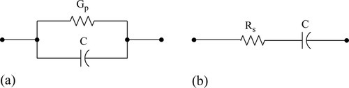

The loss factor tanδ or the dissipation factor DF = tanδ – which is frequency dependent – is defined for the parallel connection

and for the series connection
Most AC capacitors have two types of losses:
• conduction loss caused by the flow of the actual charge through the dielectric, and
• dielectric loss due to the movement or rotation of the atoms or molecules of the dielectric in an alternating electric field.
The two equivalent circuits can be combined and expanded to the single equivalent circuit of Fig. 5.7, where Ls = ESL = equivalent series inductance, Rs = ESR = equivalent series resistance, and Rp = EPR = equivalent parallel resistance. For most power system applications such a detailed equivalent circuit is not required. This circuit indicates that every capacitor has a self-resonant frequency, above which it becomes an inductor. Rs is readily measured by applying this frequency to a capacitor, measuring voltage and current, and calculating their ratio. The resistance Rp will always be much larger than the capacitive reactance at the resonant frequency and therefore this parallel resistance can be neglected at this resonant frequency.

The presence of voltage distortion increases the dielectric loss of capacitors; the total loss is for the frequency-dependent loss factor tanδh = RshωhC at hmax harmonic voltages:

where ωh = 2 · π · fh and Vh is the rms voltage of the hth harmonic. For capacitors used for low-frequency applications the relation becomes

For 60 Hz applications inexpensive AC capacitors can be used, whereas for power electronics applications and filters low-loss (e.g., ceramic or polypropylene) capacitors must be relied on.
5.7.1 Application Example 5.9: Harmonic Losses of Capacitors
For a capacitor with C = 100 μF, Vrat = 460 V, Rs1 = 0.01 Ω (where Rs1 is the series resistance of the capacitor at fundamental (h = 1) frequency of frat = 60 Hz), compute the total harmonic losses for the harmonic spectra of Table E5.9.1 (up to and including the 19th harmonic) for the following conditions:
Table E5.9.1
Possible Voltage Spectra and Associated Capacitor Losses
| h | Ph for part a (mW) | Ph for part b (mW) | Ph for part c (mW) | Ph for part a (mW) | Ph for part b (mW) | Ph for part c (mW) | ||
| 1 | 100 | 3005 | 3005 | 3005 | 100 | 3005 | 3005 | 3005 |
| 2 | 0.5 | 0.3 | 0.6 | 1.2 | 0.5 | 0.3 | 0.6 | 1.2 |
| 3 | 4.0 | 40 | 120 | 360 | 2.0a | 10.8 | 32.4 | 97.2 |
| 4 | 0.3 | 0.4 | 1.6 | 6.4 | 0.5 | 1.2 | 4.8 | 19.2 |
| 5 | 3.0 | 67.7 | 339 | 1695 | 5.0 | 188 | 940 | 4700 |
| 6 | 0.2 | 0.43 | 2.6 | 15.6 | 0.2 | 0.43 | 2.6 | 15.6 |
| 7 | 2.0 | 58.9 | 412 | 2880 | 3.5 | 181 | 1267 | 8869 |
| 8 | 0.2 | 0.77 | 6.16 | 49.3 | 0.2 | 0.77 | 6.16 | 49.3 |
| 9 | 1.0 | 24.4 | 220 | 1980 | 0.3 | 2.19 | 19.71 | 177.4 |
| 10 | 0.1 | 0.3 | 3 | 30 | 0.1 | 0.3 | 3 | 30 |
| 11 | 1.5 | 81.9 | 900 | 9900 | 1.5 | 81.9 | 900 | 9900 |
| 12 | 0.1 | 0.433 | 5.2 | 62.4 | 0.1 | 0.433 | 5.2 | 62.4 |
| 13 | 1.5 | 114 | 1480 | 19240 | 1.0 | 114 | 1482 | 19270 |
| 14 | 0.1 | 0.59 | 8.26 | 115.6 | 0.05 | 0.15 | 2.58 | 28.81 |
| 15 | 0.5 | 16.9 | 254 | 3810 | 0.1 | 0.68 | 10.2 | 153.0 |
| 16 | 0.05 | 0.192 | 3.07 | 49.1 | 0.05 | 0.192 | 3.07 | 49.1 |
| 17 | 1.0 | 87 | 1480 | 25140 | 0.5 | 22 | 374 | 6358 |
| 18 | 0.05 | 0.244 | 4.4 | 79.2 | 0.01 | 0.0097 | 0.175 | 3.143 |
| 19 | 1.0 | 109 | 2070 | 39200 | 0.5 | 27.1 | 513 | 9750 |
| All higher voltage harmonics < 0.5% | ||||||||

a Under certain conditions (e.g., DC bias of transformers as discussed in Chapter 2, and the harmonic generation of synchronous generators as outlined in Chapter 4) triplen harmonics are not of the zero-sequence type and can therefore exist in a three-phase system.
a) Rsh is constant, that is, Rsh = Rs1 = 0.01 Ω.
b) Rsh is proportional to frequency, that is, Rsh = Rs1(f/frat) = 0.01·h Ω.
c) Rsh is proportional to the square of frequency, Rsh = Rs1(f/frat)2 = 0.01·h2 Ω.
Solution to Application Example 5.9
Single-Phase System
The application of Eq. 5–19 for h = 1 yields the fundamental loss for the single-phase system at Rs1 = 0.01 Ω,
P1 = (100·10− 6)2(0.01)[(377)(1)]2(460)2 = 3005 mW.
For h = hmax = 19, Eq. 5–19 results for the single-phase system and Rs1 = 0.01 Ω in the loss P19 = (100·10− 6)2(0.01)[(377)(19)]2(4.6)2 = 109 mW.
a) The total harmonic losses including the fundamental loss is for the single-phase system at Rsh = 0.01 Ω, Ptotal_single-phase = 3.608 W.
b) The total harmonic losses including the fundamental loss is for the single-phase system at Rsh = 0.01·h Ω, Ptotal_single-phase = 10.035 W.
c) The total harmonic losses including the fundamental loss is for the single-phase system at Rsh = 0.01·h2 Ω, Ptotal_single-phase = 107.62 W.
Fundamental and harmonic losses for the single-phase system are listed in columns 3–5 of Table E5.9.1.
Three-Phase System
The application of Eq. 5–19 for h = 1 yields the fundamental loss for the three-phase system provided the capacitor bank is in Δ-connection at Rs1 = 0.01 Ω, P1 = (100·10− 6)2(0.01) [(377)(1)]2(460)2 = 3005 mW.
For h = hmax = 19 Eq. 5–19 results for the three-phase system at Rs1 = 0.01 Ω, P19 = (100·10− 6)2(0.01) [(377)(19)]2(2.3)2 = 27.1 mW.
a) The total harmonic losses including the fundamental loss is for the three-phase system at Rsh = 0.01 Ω, Ptotal_three-phase = 3.636 W.
b) The total harmonic losses including the fundamental loss is for the three-phase system at Rsh = 0.01·h Ω, Ptotal_three-phase = 8.571 W.
c) The total harmonic losses including the fundamental loss is for the three-phase system at Rsh = 0.01·h2 Ω, Ptotal_three-phase = 62.54 W.
Fundamental and harmonic losses for the three-phase system are listed in columns 7–9 of Table E5.9.1.
Conclusion
The results of this application example stress that the harmonic losses of capacitors are indeed one of the reasons why the higher order harmonic voltage amplitudes must be limited as recommended in Table E5.9.1.
5.8 Summary
Capacitors are important components within a power system: they are indispensable for voltage control, power-factor correction, and the design of filters. Their deployment may cause problems associated with capacitor switching and series resonance. Capacitor failures are induced by too large voltage, current, and reactive power harmonics. In most cases triplen (multiples of 3) and even harmonics do not exist in a three-phase system. However, there are conditions where triplen harmonics are not of the zero-sequence type and they can occur within three-phase systems. Triplen harmonics are mostly dominant in single-phase systems, whereas even harmonics are mostly negligibly small within single- and three-phase systems. In this chapter the difference between displacement power factor (DPF) – pertaining to fundamental quantities only – and the concept of the total power factor (TPF) – pertaining to fundamental and harmonic quantities – is explained. For the special case when there are no harmonics present these two factors will be identical; otherwise, the TPF is always smaller than the DPF. The TPF concept is related to the distortion power D and the DPF and TPF must be in power systems of the lagging type if consumer notation for the current is assumed. Leading power factors tend to cause oscillations and instabilities within power systems.
The losses of capacitors can be characterized by the loss factor or dissipation factor (DF) = tanδ, which is a function of the harmonic frequency. AC capacitor losses are computed for possible single- and three-phase voltage spectra.
5.9 Problems
Problem 5.1: Calculation of Displacement Power Factor (DPF) and its Correction
A VL-L = 460 V, f = 60 Hz, p = 6 pole, nm = 1180 rpm, Y-connected squirrel-cage induction motor has the following parameters per phase referred to the stator:
RS = 0.19 Ω, XS = 0.75 Ω, Xm = 20 Ω, Rʹr = 0.070 Ω, Xʹr = 0.380 Ω, and Rfe → ∞.
a) Calculate the full-load current Ĩs and the displacement power factor cosφ of the motor (without capacitor bank).
b) In Fig. P5.1 the reactive current component of the motor is corrected by a capacitor bank Cbank. Find Cbank such that the DPF as seen at the input of the capacitor is DPF = cosφ = 0.98 lagging based on the consumer notation of current flow.

Problem 5.2: Calculation of the Total Power Factor (TPF) and the DPF Correction
The following problem studies the power-factor correction for a relatively weak power system where the difference between the displacement power factor (DPF) and the total power factor (TPF) is large due to the relatively large amplitudes of voltage and current harmonics.
a) Perform a PSpice analysis for the circuit of Fig. P5.2, where a three-phase diode rectifier – fed by a Y/Y transformer with turns ratio Np/Ns = 1 – is combined with a self-commutated switch (e.g., metal-oxide-semiconductor field-effect transistors (MOSFET) or insulated-gate bipolar transistor (IGBT)) and a filter (e.g., capacitor Cf) serving a load (Rload). You may assume Rsyst = 0.1 Ω, Xsyst = 0.5 Ω, f = 60 Hz, vAN (t) = ![]() ·346 V cosωt, vBN (t) =
·346 V cosωt, vBN (t) = ![]() ·346 V cos(ωt − 120°), vCN (t) =
·346 V cos(ωt − 120°), vCN (t) = ![]() · 346 V cos(ωt – 240°), ideal diodes D1 to D6, Cf = 500 μF, Rload = 10 Ω, and a switching frequency of the self-commutated switch of fsw = 600 Hz at a duty cycle of δ = 50%. Plot one period of the voltage and current after steady state has been reached as requested in parts b and c.
· 346 V cos(ωt – 240°), ideal diodes D1 to D6, Cf = 500 μF, Rload = 10 Ω, and a switching frequency of the self-commutated switch of fsw = 600 Hz at a duty cycle of δ = 50%. Plot one period of the voltage and current after steady state has been reached as requested in parts b and c.

b) Plot and subject the line-to-neutral voltage van(t) to a Fourier analysis.
c) Plot and subject the phase current ia(t) to a Fourier analysis.
d) Repeat parts a to c for δ = 10%, 20%, 30%, 40%, 60%, 70%, 80%, and 90%.
e) Calculate the DPF = cosφ and the TPF = cosθ based on the phase shifts of the fundamental and harmonics between van(t) and ia(t) for all duty cycles and plot the DPF and TPF as a function of δ.
f) Determine the capacitance (per phase) Cbank of the power-factor correction capacitor bank such that the DPF as seen by the power systems is for δ = 50% about equal to DPF = 0.95 lagging.
Problem 5.3: Relation between Total and Displacement Power Factors
For the circuit of Fig. E5.1.1 (without taking into account power-factor correction capacitors), calculate with PSpice the Fourier components (magnitude and phase) of the phase voltage van(t) and the phase current ia(t) up to the 10th harmonic. Compute and plot the ratio TPF/DPF as a function of the firing angle α.
Problem 5.4: Design of a Tuned Passive Filter
A harmonic LC filter (consisting of a capacitor and a tuning reactor) is to be designed in parallel to a power-factor correction (PFC) capacitor to improve the power quality (as recommended by IEEE-519 [8]) and to improve the DPF = cosφ from 0.5 lagging to 0.95 lagging (consumer notation). Data obtained from a harmonic analyzer at 100% loading are 6.35 kV/phase, 600 kW/phase, THD i = 26.46%, fundamental frequency f = 50 Hz, and fifth harmonic (300 Hz) current I5 = 50 A. It is desirable to reduce the THD i to 10% for Zsystem(5) = j0.1 Ω.
Problem 5.5: Harmonic Resonance
Figure E5.3.1 part (a) shows a simplified industrial power system (Rsys = 0.01 Ω, Lsys = 0.05 mH) with a power-factor correction capacitor (Cpf = 2000 μF). Industrial loads may have nonlinear (v–i) characteristics that can be approximately modeled as (constant) decoupled harmonic current sources. The utility voltages in industrial distribution systems are often distorted due to the neighboring loads and can be approximately modeled as decoupled harmonic voltage sources:

Compute frequencies of the series and parallel resonances and the harmonic currents injected into the capacitor, and plot its frequency response.
Problem 5.6: Parallel Harmonic Resonance
In the system of Fig. E5.4.1 part (a), the source has the ratio X/R = 20. Assume X/R = 2000 (losses 0.5 W/kVAr) and X/R = 10,000 (losses 0.1 W/kVAr) for low-voltage and medium-voltage high-efficiency capacitors, respectively. The harmonic current source is a six-pulse converter injecting harmonic currents of the order
where n is an integer (typically from 1 to 4) and k is the number of pulses (e.g., equal to 6 for a six-pulse converter). Find the resonance frequency of this circuit. Plot the frequency response and current amplification at bus 1.
Problem 5.7: Series Harmonic Resonance
An example of a series resonance system is demonstrated in Fig. E5.5.1 part (a), where S = 200 MVA, X/R = 20, Vbus-rms = 7.2 kV, XL = 1 Ω, QC = 900 kVAr, VCrms = 7.2 kV, ILrms = 100 A, and Z = (R + j0.049 Ω) with R = 0 and magnitude Zmag = 0.049 Ω at h = 7.59. The equivalent circuit (neglecting resistances) is shown in Fig. E5.5.1 part (b). Find the resonance frequency of this circuit. Plot the frequency response of the bus 1 equivalent impedance, and the current amplification across the tuning reactor.
Problem 5.8: Protection of Capacitors by Virtual Harmonic Resistors
Repeat Application Example 5.3 assuming a power converter is used to include a virtual harmonic resistor Rvir = 1.0 Ω in series with the capacitor.
Problem 5.9: Harmonic Current, Voltage, and Reactive Power Limits for Capacitors when Used in a Single-Phase System
The reactance of a capacitor decreases with frequency and therefore the capacitor acts as a sink for higher harmonic currents. The effect is to increase the heating and dielectric stress. ANSI/IEEE [10], IEC, and European [e.g., 11,12] standards provide limits for voltage, currents, and reactive power of capacitor banks. This can be used to determine the maximum allowable harmonic levels. The result of the increased heating and voltage stress brought about by harmonics is a shortened capacitor life due to premature aging.
According to the nameplate of the capacitors the following constraints must be satisfied:


where Vrrms_rat is the rated terminal voltage, Vrms is the applied effective (rms) terminal voltage, f1 is the line frequency, and V1 is the fundamental (rms) voltage.
Plot for Vrms ≈ Vrms_rat and f1 = frat the loci for Vh/Vrms, where (Vrms/Vrms_rat) = 1.15, (Irms/Irms_rat) = 1.3, and (Q/Qrat) = 1.45 as a function of the harmonic order h for 3 ≤ h ≤ 49 (only one harmonic is present at any time).
Problem 5.10: Harmonic Losses of Capacitors
For a capacitor with C = 100 μF, Vrat = 1000 V, Rs1 = 0.005 Ω (where Rs1 is the series resistance of the capacitor at fundamental (h = 1) frequency of frat = 60 Hz), compute the total harmonic losses for the harmonic spectra of Table P5.10 (up to and including the 19th harmonic) for the following conditions:
Table P5.10
Possible Voltage Spectra with High Harmonic Penetration
| h | ||
| 1 | 100 | 100 |
| 2 | 2.5 | 0.5 |
| 3 | 5.71 | 1.0a |
| 4 | 1.6 | 0.5 |
| 5 | 1.25 | 7.0 |
| 6 | 0.88 | 0.2 |
| 7 | 1.25 | 5.0 |
| 8 | 0.62 | 0.2 |
| 9 | 0.96 | 0.3 |
| 10 | 0.66 | 0.1 |
| 11 | 0.30 | 2.5 |
| 12 | 0.18 | 0.1 |
| 13 | 0.57 | 2.0 |
| 14 | 0.10 | 0.05 |
| 15 | 0.10 | 0.1 |
| 16 | 0.13 | 0.05 |
| 17 | 0.23 | 1.5 |
| 18 | 0.22 | 0.01 |
| 19 | 1.03 | 1.0 |
| All higher harmonics < 0.2% | ||

a Under certain conditions (e.g., DC bias of transformers as discussed in Chapter 2, and the harmonic generation of synchronous generators as outlined in Chapter 4) triplen harmonics are not of the zero-sequence type, and they can therefore exist in a three-phase system.
a) Rsh is constant, that is, Rsh = Rs1 = 0.005 Ω.
b) Rsh is proportional to frequency, that is, ![]()
c) Rsh is proportional to the square of frequency, ![]()
d) Plot the calculated losses of parts a to c as a function of the harmonic order h.