
Harmonic Models of Transformers
Abstract
Investigates the behaviour of power transformers under harmonic voltages and currents: sinusoidal transformer models suitable for harmonic loss calculations and harmonic power flow; techniques for the computation of transformer derating such as K and FHL-factors based on direct-loss measurements. Transformer harmonic models, state-space formulations and finite-difference magnetic field modelling techniques are presented. Ferroresonance, geomagnetically induced currents (GICs), transformer grounding, and surge protection issues are addressed next. Grounding techniques, derating of three-phase transformers, and the accurate loss measurement based on the direct-loss measurement approach are explained, even when the efficiency of a transformer is higher than 96% and the conventional Pin-Pout method does not yield accurate results. 10 application examples with solutions and 11 application-oriented problems are listed.
Extensive application of power electronics and other nonlinear components and loads creates single-time (e.g., spikes) and periodic (e.g., harmonics) events that could lead to serious problems within power system networks and its components (e.g., transformers). Some possible impacts of poor power quality on power transformers are
• saturating transformer core by changing its operating point on the nonlinear λ – i curve,
• increasing core (hysteresis and eddy current) losses and possible transformer failure due to unexpected high losses associated with hot spots,
• increasing (fundamental and harmonic) copper losses,
• creating half-cycle saturation in the event of even harmonics and DC current,
• malfunctioning of transformer protective relays,
• aging and reduction of lifetime,
• reduction of efficiency,
• derating of transformers,
• decrease of the power factor,
• generation of parallel (harmonic) resonances and ferroresonance conditions, and
• deterioration of transformers’ insulation near the terminals due to high voltage stress caused by lightning and pulse-width-modulated (PWM) converters.
These detrimental effects call for the understanding of how harmonics affect transformers and how to protect them against poor power quality conditions. For a transformer, the design of a harmonic model is essential for loss calculations, derating, and harmonic power flow analysis.
This chapter investigates the behavior of transformers under harmonic voltage and current conditions, and introduces harmonic transformer models suitable for loss calculations, harmonic power flow analysis, and computation of derating functions. After a brief introduction of the conventional (sinusoidal) transformer model, transformer losses with emphasis on the impacts of voltage and current harmonics are presented. Several techniques for the computation of single-phase transformer derating factors (functions) are introduced. Thereafter, a survey of transformer harmonic models is given. In subsequent sections, the issues of ferroresonance, geomagnetically induced currents (GICs), and transformer grounding are presented. A section is also provided for derating of three-phase transformers.
2.1 Sinusoidal (linear) modeling of transformers
Transformer simulation under sinusoidal operating conditions is a well-researched subject and many steady-state and transient models are available. However, transformer cores are made of ferromagnetic materials with nonlinear (B–H) or (λ – i) characteristics. They exhibit three types of nonlinearities that complicate their analysis: saturation effect, hysteresis (major and minor) loops, and eddy currents. These phenomena result in nonsinusoidal flux, voltage and current waveforms on primary and secondary sides, and additional copper (due to current harmonics) and core (due to hysteresis loops and eddy currents) losses at fundamental and harmonic frequencies. Linear techniques for transformer modeling neglect these nonlinearities (by assuming a linear (λ – i) characteristic) and use constant values for the magnetizing inductance and the core-loss resistance. Some more complicated models assume nonlinear dependencies of hysteresis and eddy-current losses with fundamental voltage magnitude and frequency, and use a more accurate equivalent value for the core-loss resistance. Generally, transformer total core losses can be approximated as
where Phys, Peddy, Bmax, and f are hysteresis losses, eddy-current losses, maximum value of flux density, and fundamental frequency, respectively. Khys is a constant for the grade of iron employed and Keddy is the eddy-current constant for the conductive material. S is the Steinmetz exponent ranging from 1.5 to 2.5 depending on the operating point of transformer core.
Transient models are used for transformer simulation during turning-on (e.g., inrush currents), faults, and other types of disturbances. They are based on a system of time-dependent differential equations usually solved by numerical algorithms. Transient models require a considerable amount of computing time. Steady-state models mostly use phasor analysis in the frequency domain to simulate transformer behavior, and require less computing times than transient models. Transformer modeling for sinusoidal conditions is not the main objective of this chapter. However, Fig. 2.1 illustrates a relatively simple and accurate frequency-based linear model that will be extended to a harmonic model in Section 2.4. In this figure Rc is the core-loss resistance, Lm is the (linear) magnetizing inductance, and Rp, R′s Lp, and L′s are transformer primary and secondary resistances and inductances, respectively. Superscript ′ is used for quantities referred from the secondary side to the primary side of the transformer.

The steady-state model of Fig. 2.1 is not suitable for harmonic studies since constant values are assumed for the magnetizing inductance and the core-loss resistance. However, this simple and practical frequency-based model generates acceptable results if a transformer were to operate in the linear region of the (λ – i) characteristic, and the harmonic frequency is taken into account.
2.2 Harmonic losses in transformers
Losses due to harmonic currents and voltages occur in windings because of the skin effect and the proximity effect. It is well known that harmonic current ih(t) and harmonic voltage vh(t) must be present in order to produce harmonic losses
If either ih(t) or vh(t) are zero then ph(t) will be zero as well. Harmonic losses occur also in iron cores due to hysteresis and eddy-current phenomena. For linear (B–H) characteristics of iron cores, the losses are dependent on fundamental and harmonic amplitudes only, whereas for nonlinear iron-core (B–H) characteristics (Fig. 2.2) the phase shift between harmonic voltage and fundamental voltage is important as well. For example, a magnetizing current with maximum peak-to-peak values results in larger maximum flux densities than a magnetizing current with minimum peak-to-peak values. Proximity losses in windings and (solid) conducting parts of a device (e.g., frame) occur due to the relative location between the various windings and conductive parts.

2.2.1 Skin Effect
If a conductor with cross section acond conducts a DC current IDC, the current density jDC = IDC/acond is uniform within the conductor and a resistance RDC can be assigned to the conductor representing the ratio between the applied voltage VDC and the resulting current IDC, that is,

For (periodic) AC currents iACh(t), the current flows predominantly near the surface of the conductor and the current density jACh is nonuniform within the conductor (Fig. 2.3). In general, RDC < RACh. The higher the order h of the harmonic current iACh(t), the larger is the skin effect.

2.2.2 Proximity Effect
The AC current distribution within a conductor depends on the current distribution of neighboring conductors or conducting parts. The AC field ![]() of a single conductor in free space consists of circles symmetric to the axis of the conductor. Ampere’s law
of a single conductor in free space consists of circles symmetric to the axis of the conductor. Ampere’s law

If there are two conductors or more, the circular fields will be distorted and the resulting eddy-current losses within the conductor will differ from those of single conductors. In Figs. 2.4 and 2.5, H stands for ![]() .
.


2.2.3 Magnetic Iron-Core (Hysteresis and Eddy-Current) Losses
All magnetic materials exhibit saturation and hysteresis properties: there are major loops and minor loops (Fig. 2.6) and such characteristics are multivalued for either a single H or a single B value.

Therefore, even if there is a sinusoidal input voltage to a magnetic circuit and no minor (B–H) loops are assumed, a nonsinusoidal current and increased losses are generated. For nonsinusoidal excitation and/or nonlinear loads, excessive magnetic and (fundamental and harmonic) copper losses may result that could cause transformer failure. In most cases hysteresis losses can be neglected because they are relatively small as compared with copper losses. However, the nonlinear saturation behavior must be taken into account because all transformers and electric machines operate for economic reasons beyond the knee of saturation.
Faraday’s law

or

is valid, where e(t) is the induced voltage of a winding residing on an iron core, λ(t) = NΦ(t) are the flux linkages, N is the number of turns of a winding, and Φ(t) is the flux linked with the winding.
Depending on the phase shift of a harmonic voltage with respect to the fundamental voltage the resulting wave shape of the flux linkages will be different and not proportional to the resulting voltage wave shape due to the integral relationship between flux linkages λ(t) and induced voltage e(t) [1–6].
2.2.3.1 Application Example 2.1: Relation between Voltages and Flux Linkages for 0° Phase Shift between Fundamental and Harmonic Voltages
If the third harmonic voltage e3(t) is in phase (0°) with the fundamental voltage e1(t) results in a maximum peak-to-peak value for the total nonsinusoidal voltage. According to Eq. 2-6, the peak-to-peak value of the generated λ(t) is then minimum, as illustrated by Fig. E2.1.1.

Rule
A “peaky” (peak-to-peak is maximum) voltage {e1(t) + e3(t)} results in “flat” (peak-to-peak is minimum) flux linkages.
2.2.3.2 Application Example 2.2: Relation between Voltages and Flux Linkages for 180° Phase Shift between Fundamental and Harmonic Voltages
If the third harmonic voltage e3(t) is out of phase (180°) with the fundamental voltage e1(t) then the total voltage and the resulting flux linkages have minimum and maximum peak-to-peak values, respectively (Fig. E2.2.1).

Rule
A “flat” (peak-to-peak is minimum) voltage {e1(t) + e3(t)} results in “peaky” (peak-to-peak is maximum) flux linkages.
Generalization
For higher harmonic orders, similar relations between the nonsinusoidal waveforms of induced voltage and flux linkages exist; however, there is an alternating behavior as demonstrated in Table E2.2.1.
Table E2.2.1
Phase Relations between Induced Voltages and Flux Linkages when a Harmonic is Superposed with the Fundamental
| Harmonic order | Nonsinusoidal voltage e1(t) + eh(t) | Nonsinusoidal flux linkage |
| h = 3 | {e1(t) + e3(t)} peakya | |
| {e1(t) + e3(t)} flat | ||
| h = 5 | {e1(t) + e5(t)} peaky | |
| {e1(t) + e5(t)} flat | ||
| h = 7 | {e1(t) + e7(t)} peaky | |
| {e1(t) + e7(t)} flat | ||
| h = 9 | {e1(t) + e9(t)} peaky | |
| {e1(t) + e9(t)} flat | ||

a Maximum peak-to-peak value.
b Minimum peak-to-peak value.
This alternating behavior (due to the integral relationship between e(t) and λ(t)) influences the iron-core (magnetic) losses significantly. Therefore, it is possible that a nonsinusoidal voltage results in less iron-core losses than a sinusoidal wave shape [2]. Note that the iron-core losses are a function of the maximum excursions of the flux linkages (or flux densities Bmax).
2.2.4 Loss Measurement
For low efficiency (η < 97%) devices (e.g., transformers) the conventional indirect loss measurement approach, where the losses Ploss are the difference between measured input power Pin and measured output power Pout, is acceptable. However, for high efficiency (η ≥ 97%) devices the indirect loss measurement approach yields losses that have a large error.
2.2.4.1 Indirect Loss Measurement
Consider the two-port system shown in Fig. 2.7:
or

This is the conventional and relatively simple (indirect) technique used for loss measurements of most low-efficiency electric devices under sinusoidal and/or nonsinusoidal operating conditions.

2.2.4.2 Direct Loss Measurement
The two port system of Fig. 2.7 can be specified in terms of series and shunt impedances [1–6], as illustrated in Fig. 2.8.

The powers dissipated in Zseries1 and Z’series2 are

The power dissipated in Zshunt is

Therefore,
2.2.4.3 Application Example 2.3: Application of the Direct-Loss Measurement Technique to a Single-Phase Transformer
The direct-loss measurement technique is used to measure losses of a single-phase transformer as illustrated in Fig. E2.3.1 [7].

Solution to Application Example 2.3
Transformer losses are

Rearrangement of terms results in


Note that Ploss consists of the sum (not the difference) of two components where (v1 – v2′) and (i1 – i2′) can be accurately measured and calibrated. Thus the difference of Pin and Pout is not computed as for the indirect, conventional method of Section 2.2.4.1. This method can be applied to polyphase systems as discussed in [8,9]. The two available sampling methods – series and parallel sampling – are addressed in Appendix 1.
2.3 Derating of single-phase transformers
According to the IEEE dictionary, derating is defined as “the intentional reduction of stress/strength ratio (e.g., real or apparent power) in the application of an item (e.g., transformer), usually for the purpose of reducing the occurrence of stress-related failure (e.g., reduction of lifetime of transformer due to increased temperature beyond rated temperature).” As has been discussed in Section 2.2 harmonic currents and voltages result in harmonic losses increasing the temperature rise. This rise beyond its rated value results in a reduction of lifetime [10] as will be discussed in Chapter 6. For transformers two derating parameters can be defined:
• reduction in apparent power rating (RAPR), and
• real power capability (RPC).
Although the first one is independent of the power factor, the second one is strongly influenced by it.
2.3.1 Derating of Transformers Determined from Direct-Loss Measurements
The direct-loss measurement technique of Section 2.2.4.2 is applied and the reduction of apparent power (RAPR) is determined such that for any given total harmonic distortion of the current (THDi), the rated losses of the transformer will not be exceeded. Figures 2.9 and 2.10 show the RAPR and RPC as a function of the THDi.


2.3.2 Derating of Transformers Determined from the K-Factor
It is well known that power system transformers must be derated when supplying nonlinear loads. Transformer manufacturers have responded to this problem by developing transformers rated for 50% or 100% nonlinear load. However, the impact of nonlinear loads on transformers greatly depends on the nature and the harmonic spectrum caused by the nonlinear load, which is not considered by the manufacturers. The K-factor rating is an alternative technique for transformer derating that includes load characteristics [11,13].
The assumptions used in calculating K-factor can be found in ANSI/IEEE C57.110, IEEE Recommended Practice for Establishing Transformer Capability when Supplying Nonsinusoidal Load Currents [13,14]. This recommendation calculates the harmonic load current that causes losses equivalent to the rated (sinusoidal) load current so that the transformer’s “hot spot” temperature will not be exceeded. The hot spot is assumed to be where eddy-current losses are the greatest and the coolant (oil) is hottest (e.g., at the inner low-voltage winding).
The load loss (LL) generating the hot spot temperature is assumed to consist of I2R and eddy-current PEC losses:
The eddy current losses (Eq. 2–12) are proportional to the square of the current and frequency:
where KEC is a proportionality constant. Under rated (sinusoidal) conditions, the load loss resulting in the hot spot temperature can be expressed as
where PEC–R is the eddy-current loss resulting in the hot spot temperature under rated (sinusoidal) operating conditions. In per unit of the rated I2R loss, Eq. 2-14 becomes
Therefore, the transformer load loss under harmonic conditions is

The first and second terms on the right side of the above equation represent the I2R loss and the eddy-current loss, respectively. Setting PLL = PLL–R gives

Now, if we define the K-factor as follows [13]:
then

Solving for 

Therefore, the maximum amount of rms harmonic load current that the transformer can deliver is

Using the K-factor and transformer parameters, the maximum permissible rms current of the transformer can also be defined as follows [11]:
RDC = RDCprimary + RʹDCsecondary is the total DC resistance of a transformer winding. REC–R is the rated additional resistance due to eddy currents. In addition,

and

ΔPfe is the difference between the total iron core losses (including harmonics) and the rated iron core losses without harmonics. ΔPOSL is the difference between the total other stray losses (OSL) including harmonics and the rated other stray losses without harmonics.
The reduction of apparent power (RAPR) is
where V2rmsnonlinear and V2rmsrat are the total rms value of the secondary voltage including harmonics and the rated rms value of the secondary winding without harmonics, respectively. All above parameters are defined in [11].
2.3.3 Derating of Transformers Determined from the FHL-Factor
The K-factor has been devised by the Underwriters Laboratories (UL) [13] and has been recognized as a measure for the design of transformers feeding nonlinear loads demanding nonsinusoidal currents. UL designed transformers are K-factor rated. In February 1998 the IEEE C57.110/D7 [14] standard was created, which represents an alternative approach for assessing transformer capability feeding nonlinear loads. Both approaches are comparable [15].
The FHL-factor is defined as

Thus the relation between K-factor and FHL-factor is

or the maximum permissible current is [15]

and the reduction in apparent power rating (RAPR) is

The RAPR as a function of THDi is shown in Fig. 2.11.

2.3.3.1 Application Example 2.4: Sensitivity of K- and FHL-Factors and Derating of 25 kVA Single-Phase Pole Transformer with Respect to the Number and Order of Harmonics
The objective of this example is to show that the K-and FHL-factors are a function of the number and order of harmonics considered in their calculation.
The harmonic content of a square wave with magnitude 1.00 pu is known.
a) Develop a Fourier analysis program for any periodic function resulting in the DC offset and the amplitudes of any even and odd harmonics involved.
b) Apply this program to a square wave with magnitude 1.00 pu by taking into account the Nyquist criterion.
c) Plot the original square wave and its Fourier approximation.
d) Compute the K- and FHL-factors by taking various numbers and orders of harmonics into account.
Solution to Application Example 2.4
a) The Fourier analysis program is listed in Appendix A2.1.
b) Output of the Fourier program for a square wave is listed in Appendix A2.2.
c) Taking into account the Nyquist criterion one can compute based on 42 sampled points per period the harmonics up to the 27th order. These harmonics are listed in Table E2.4.1 and the resulting Fourier approximation is shown in Fig. E2.4.1.
Table E2.4.1
Spectrum of Square Wave
| IDC (pu) | I1 (pu) | I2 (pu) | I3 (pu) | I4 (pu) | I5 (pu) | I6 (pu) |
| 0 | 1.27 | 0.04 | 0.42 | 0.04 | 0.25 | 0.04 |
| I7 (pu) | I8 (pu) | I9 (A) | I10 (pu) | I11 (pu) | I12 (pu) | I13 (pu) |
| 0.17 | 0.04 | 0.12 | 0.04 | 0.09 | 0.04 | 0.07 |
| I14 (pu) | I15 (pu) | I16 (pu) | I17 (pu) | I18 (pu) | I19 (pu) | I20 (pu) |
| 0.04 | 0.05 | 0.03 | 0.04 | 0.03 | 0.03 | 0.04 |
| I21 (pu) | I22 (pu) | I23 (pu) | I24 (pu) | I25 (pu) | I26 (pu) | I27 (pu) |
| 0.04 | 0.03 | 0.03 | 0.02 | 0.03 | 0.02 | 0.03 |
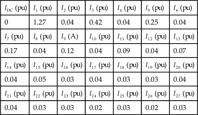

 ) represent sampled values and the continuously drawn function represents the Fourier approximation. Note that 1A corresponds to 1 pu.
d) Taking into account the harmonics up to the 27th order (Table E2.4.2) one obtains for the K-factor: K27 = 9.86, and for the FHL-factor: FHL27 = 8.22. Thereby it is assumed that the 25 kVA single-phase pole transformer [11] is loaded only by nonlinear loads having square wave currents. Using these factors and knowing the PEC-R, one can compute the derating of a transformer. The PEC-R can be obtained from the manufacturer or it can be measured [11]. For PEC-R = 0.0186 pu one obtains using the K-factor, Eq. 2-21 the derating:
Table E2.4.2
Parameters for the Calculation of the K- and FHL-Factors (Note the Values for the Ih (pu) are Truncated)
| h | Ih (pu) | Ih2 | h2Ih2 |
| 1 | 1.0 | 1.0 | 1.0 |
| 2 | 0.03 | 0.001 | 0.004 |
| 3 | 0.33 | 0.109 | 0.984 |
| 4 | 0.03 | 0.001 | 0.016 |
| 5 | 0.20 | 0.040 | 0.969 |
| 6 | 0.03 | 0.001 | 0.036 |
| 7 | 0.13 | 0.018 | 0.878 |
| 8 | 0.03 | 0.001 | 0.063 |
| 9 | 0.09 | 0.009 | 0.723 |
| 10 | 0.03 | 0.001 | 0.099 |
| 11 | 0.07 | 0.005 | 0.608 |
| 12 | 0.03 | 0.001 | 0.143 |
| 13 | 0.06 | 0.003 | 0.513 |
| 14 | 0.03 | 0.001 | 0.194 |
| 15 | 0.04 | 0.002 | 0.349 |
| 16 | 0.02 | 0.0006 | 0.143 |
| 17 | 0.03 | 0.001 | 0.287 |
| 18 | 0.02 | 0.0006 | 0.181 |
| 19 | 0.02 | 0.0006 | 0.201 |
| 20 | 0.03 | 0.001 | 0.397 |
| 21 | 0.03 | 0.001 | 0.438 |
| 22 | 0.02 | 0.0006 | 0.270 |
| 23 | 0.02 | 0.0006 | 0.295 |
| 24 | 0.02 | 0.0002 | 0.143 |
| 25 | 0.02 | 0.0006 | 0.348 |
| 26 | 0.02 | 0.0002 | 0.168 |
| 27 | 0.02 | 0.0006 | 0.407 |
| Σ | 1.2006 | 9.860 |

and the derating based on the FHL-factor, with Eqs. 2-21, Eqs. 2-24 and Eq. 2-25:

Conclusion
The calculation of the derating of transformers with the K- and FHL-factors leads to the same result provided the same number and order of harmonics are considered.
To show that the K- and FHL-factors and, therefore the derating calculation, critically depend on the number and order of harmonics (used in their calculation), in the following the number of harmonics is reduced from 27 to 13. Thus one obtains K13 = 6.04 and FHL13 = 5.08, resulting in
Conclusion
K27 > K13 and FHL27 > FHL13, therefore Imax13 (pu) > Imax27 (pu).
2.3.3.2 Application Example 2.5: K- and FHL-Factors and Their Application to Derating of 25 kVA Single-Phase Pole Transformer Loaded by Variable-Speed Drives
The objective of this example is to apply the computational procedure of Application Example 2.4 to a 25 kVA single-phase pole transformer loaded only by variable-speed drives of central residential air-conditioning systems [16]. Table E2.5.1 lists the measured current spectrum of the air handler of a variable-speed drive with (medium or) 50% of rated output power.
Table E2.5.1
Current Spectrum of the Air Handler of a Variable-Speed Drive with (Medium or) 50% of Rated Output Power
| IDC (A) | I1 (A) | I2 (A) | I3 (A) | I4 (A) | I5 (A) | I6 (A) |
| –0.82 | 10.24 | 0.66 | 8.41 | 1.44 | 7.27 | 1.29 |
| I7 (A) | I8 (A) | I9 (A) | I10 (A) | I11 (A) | I12 (A) | I13 (A) |
| 4.90 | 0.97 | 3.02 | 0.64 | 1.28 | 0.48 | 0.57 |
| I14 (A) | I15 (A) | I16 (A) | I17 (A) | I18 (A) | I19 (A) | I20 (A) |
| 0.53 | 0.73 | 0.57 | 0.62 | 0.31 | 0.32 | 0.14 |
| I21 (A) | I22 (A) | I23 (A) | I24 (A) | I25 (A) | I26 (A) | I27 (A) |
| 0.18 | 0.29 | 0.23 | 0.39 | 0.34 | 0.39 | 0.28 |

a) Plot the input current wave shape of this variable-speed drive and its Fourier approximation.
b) Compute the K- and FHL-factors and their associated derating of the 25 kVA single-phase pole transformer feeding variable-speed drives of central residential air-conditioning systems. This assumption is a worst-case condition, and it is well-known that pole transformers also serve linear loads such as induction motors of refrigerators and induction motors for compressors of central residential air-conditioning systems.
Solution to Application Example 2.5
Taking into account the harmonics up to the 27th order (Tables E2.5.1 and E2.5.2) one obtains for the K-factor: K27 = 50.52, and for the FHL-factor: FHL27 = 19.42. Using these factors and knowing the value of PEC-R one can compute the derating of a transformer. The PEC-R can be obtained from the manufacturer or it can be measured [11]. For PEC-R = 0.0186 pu one obtains the derating using the K-factor, Eq. 2-21:
and the derating based on the FHL-factor, with Eq. 2-21, Eq. 2-24 and Eq. 2-25:

Table E2.5.2
Parameters for the Calculation of the K- and FHL-Factors (Note the Values for the Ih (pu) are Rounded)
| h | Ih (pu) | Ih2 | h2Ih2 |
| 1 | 1.024 | 1.0486 | 1.0486 |
| 2 | 0.066 | 0.0044 | 0.0176 |
| 3 | 0.841 | 0.7073 | 6.3657 |
| 4 | 0.144 | 0.0207 | 0.3312 |
| 5 | 0.727 | 0.5285 | 13.2125 |
| 6 | 0.129 | 0.01664 | 0.5990 |
| 7 | 0.490 | 0.2401 | 11.7649 |
| 8 | 0.097 | 0.0094 | 0.6016 |
| 9 | 0.302 | 0.0910 | 7.3710 |
| 10 | 0.064 | 0.0041 | 0.4100 |
| 11 | 0.128 | 0.0164 | 1.9844 |
| 12 | 0.048 | 0.0023 | 0.3312 |
| 13 | 0.057 | 0.0033 | 0.5577 |
| 14 | 0.053 | 0.00281 | 0.5508 |
| 15 | 0.073 | 0.0053 | 1.1925 |
| 16 | 0.057 | 0.0033 | 0.8448 |
| 17 | 0.062 | 0.0038 | 1.0982 |
| 18 | 0.031 | 0.0010 | 0.3240 |
| 19 | 0.032 | 0.0010 | 0.3610 |
| 20 | 0.014 | 0.0002 | 0.0800 |
| 21 | 0.018 | 0.0003 | 0.1323 |
| 22 | 0.029 | 0.0008 | 0.3872 |
| 23 | 0.023 | 0.0005 | 0.2645 |
| 24 | 0.039 | 0.0015 | 0.8640 |
| 25 | 0.034 | 0.0012 | 0.7500 |
| 26 | 0.039 | 0.0015 | 1.0140 |
| 27 | 0.028 | 0.0007 | 0.5103 |
| Σ | 2.7271 | 52.9690 |

Note that the influence of the DC component of the current has been disregarded. As is shown in [9], this DC component contributes to additional AC losses and an additional temperature rise further increasing the derating.
Measured current wave shape of the air handler operating at variable speed with (medium or) 50% of rated output power with a DC component of IDC = –0.82 A is shown in Fig. E2.5.1. The corresponding Fourier approximation (based on the Fourier coefficients of Table E2.5.1) without the DC offset is compared with measured current waveform in Fig. E2.5.2. In Table E2.5.2 the fundamental current is not normalized to 1.00 pu; this does not affect the calculation of the K- and FHL-factors.


 ) represent measured (sampled) values and the continuous line is the Fourier approximation based on the Fourier coefficients of Table E2.5.2. All ordinate values must be divided by 10 to obtain pu values.
2.4 Nonlinear harmonic models of transformers
Appropriate harmonic models of all power system components including transformers are the basis of harmonic analysis and loss calculations. Harmonic models of transformers are devised in two steps: the first is the construction of transformer harmonic model, which is mainly characterized by the analysis of the core nonlinearity (due to saturation, hysteresis, and eddy-current effects), causing nonsinusoidal magnetizing and core-loss currents. The second step involves the relation between model parameters and harmonic frequencies. In the literature, many harmonic models for power transformers have been proposed and implemented. These models are based on one of the following approaches:
• time-domain simulation [17–25],
• frequency-domain simulation [26–29],
• combined frequency- and time-domain simulation [30,31], and
• numerical (e.g., finite-difference, finite-element) simulation [1,2,6,32–34].
This section starts with the general harmonic model for a power transformer and the simulation techniques for modeling its nonlinear iron core. The remainder of the section briefly introduces the basic concepts and equations involving each of the above-mentioned modeling techniques.
2.4.1 The General Harmonic Model of Transformers
Figure 2.12 presents the physical model of a single-phase transformer. The corresponding electrical and magnetic equations are


where
• Rp and Rs are the resistances of the primary and the secondary windings, respectively,
• Lp and Ls are the leakage inductances of primary and secondary windings, respectively,
• ![]() and
and ![]() are the induced voltages of the primary and the secondary windings, respectively,
are the induced voltages of the primary and the secondary windings, respectively,
• Np and Ns are the number of turns of the primary and the secondary windings, respectively,
• B, H and Φm are the magnetic flux density, the magnetic field intensity, and the magnetic flux in the iron core of the transformer, respectively, and
• A and ℓ are the effective cross section and length of the integration path of transformer core, respectively.

Dividing Eq. 2-32 by Np yields

where iexc (t) = Hℓ/Np is the transformer excitation (no-load) current, which is the sum of the magnetizing (imag(t)) and core-loss (icore(t)) currents. Combining Eqs. 2-30 and 2-31, it is clear that the no-load current is related to the physical parameters, that is, the magnetizing curve (including saturation and hysteresis) and the induced voltage.
Based on Eqs. 2-28, 2-29, and 2-33, the general harmonic model of transformer is obtained as shown in Fig. 2.13. There are four dominant characteristic parameters:

• leakage inductance,
• magnetizing current, and
• core-loss current.
Some models assume constant values for the primary and the secondary resistances. However, most references take into account the influence of skin effects and proximity effects in the harmonic model. Since primary (Φpℓ) and secondary (Φsℓ) leakage fluxes mainly flow across air, the primary and the secondary leakage inductances can be assumed to be constants. The main difficulty arises in the computation of the magnetizing and core-loss currents, which are the main sources of harmonics in power transformers.
2.4.2 Nonlinear Harmonic Modeling of Transformer Magnetic Core
Accurate transformer models incorporate nonlinear saturation and hysteresis phenomena. Numerous linear, piecewise linear, and nonlinear models are currently available in the literature for the representation of saturation and hysteresis effects of transformer cores. Most models are based on time-domain techniques that require considerable computing time; however, there are also a few frequency-based models with acceptable degrees of accuracy. It is the purpose of this section to classify these techniques and to introduce the most widely used models.
2.4.2.1 Time-Domain Transformer Core Modeling by Multisegment Hysteresis Loop
The transformer core can be accurately modeled in the time domain by simulating its (λ – i) characteristic including the major hysteresis loop (with or without minor loops), which accounts for all core effects: hysteresis loss, eddy-current loss, saturation, and magnetization (Fig. 2.14). The (λ – i) loop is divided into a number of segments and each segment is approximated by a parabola [20], a polynomial [31], a hyperbolic [25], or other functions. The functions expressing the segments must be defined so that di/dλ (or dH/dB) is continuous in the entire defined region of the (λ - i) or (B–H) plane.

As an example, two typical (λ - i) characteristics are shown in Fig. 2.15. Five segments are used in Fig. 2.15a to model the (λ – i) loop [20]. The first three are approximated by polynomials of the 13th order while the fourth and the fifth segments (in the positive and negative saturation regions) are represented by parabolas. The expression for describing the four-segment loop of Fig. 2.15b is [31]


There is a major difficulty with time-domain approaches. For a given value of maximum flux linkage, λmax the loop is easily determined experimentally; however, for variable λmax the loop not only changes its size but also its shape. Since these changes are particularly difficult to predict, the usual approach is to neglect the variation in shape and to assume linear changes in size. This amounts to scaling the characteristics in the λ and i directions for different values of λmax.
This is a fairly accurate model for the transformer core; however, it requires considerable computing time. Some more sophisticated models also include minor hysteresis loops in the time-domain analysis [27].
2.4.2.2 Frequency- and Time-Domain Transformer Core Modeling by Saturation Curve and Harmonic Core-Loss Resistances
In these models, transformer saturation is simulated in the time domain while eddy-current losses and hysteresis are approximated in the frequency domain. If the voltage that produces the core flux is sinusoidal with rms magnitude of E and frequency of f, Eq. 2-1 may be rewritten as [31]
where khys ≠ Khys and keddy ≠ Keddy.
Although the application of superposition is incorrect for nonlinear circuits, in some cases it may be applied cautiously to obtain an approximate solution. If superposition is applied, the core loss due to individual harmonic components may be defined to model both hysteresis and eddy-current losses by dividing Eq. 2-35 by the square of the rms harmonic voltages. We define the conductance Geddy (accounting for eddy-current losses) and harmonic conductance Ghys(h) (accounting for hysteresis losses at harmonic frequencies) as [31]
where f and h are the fundamental frequency and harmonic order, respectively. Therefore, eddy current (Peddy) and hysteresis (Phys) losses are modeled by a constant conductance (Geddy) and harmonic conductances (Ghys(h)), respectively, and the transformer (λ - i) characteristic is approximated by a single-valued saturation curve, as shown in Fig. 2.16 [31]. There are basically two main approaches for modeling the transformer saturation curve: piecewise linear inductances and incremental inductance [19], as shown by Fig. 2.16b,c. The incremental approach uses a polynomial [31,30], arctangent [22,23], or other functions to model the transformer magnetizing characteristic. The incremental reluctances (or inductances) are then obtained from the slopes of the inductance-magnetizing current characteristic.

2.4.2.3 Time-Domain Transformer Coil Modeling by Saturation Curve and a Constant Core-Loss Resistance
Due to the fact that the effect of hysteresis in transformers is much smaller than that of the eddy current, and to simplify the computation, most models assume a constant value for the magnetizing conductance [22,23,30]. As mentioned before, the saturation curve may be modeled using a polynomial [30,29], arctangent [22,23], or other functions. The slightly simplified transformer model is shown in Fig. 2.17.

2.4.2.4 Frequency-Domain Transformer Coil Modeling by Harmonic Current Sources
Some frequency-based algorithms use harmonic current sources (Ĩcore(h) and Ĩmag(h)) to model the nonlinear effects of eddy current, hysteresis, and saturation of the transformer core, as shown in Fig. 2.18. The magnitudes and phase angle of the current sources are upgraded at each step of the iterative procedure. There are different methods for upgrading (computing) magnitudes and phase angles of current sources at each step of the iterative procedure. Some models apply the saturation curve to compute Ĩmag(h) in the time domain, and use harmonic loss-density and so called phase-factor functions to compute Ĩcore(h) in the frequency domain [1–4,20]. These currents could also be approximately computed in the frequency domain as explained in the next section.

2.4.2.5 Frequency-Domain Transformer Coil Modeling by Describing Functions
The application of describing functions for the computation of the excitation current in the frequency domain was proposed and implemented for a single-phase transformer under no-load conditions [26]. The selected describing function, which assumes sinusoidal flux linkages and a piecewise linear hysteresis loop, is relatively fast and computes the non-sinusoidal excitation current with an acceptable degree of accuracy. The concept of describing functions as applied to the nonlinear (symmetric) network N is demonstrated in Fig. 2.19, where a sinusoidal input function λ(t) = E sin(ωt) results in a nonsinusoidal output function ie(t). Neglecting the influence of harmonics, ie(t) can be approximated as


In Eq. 2-37, A1 and B1 are the fundamental coefficients of the Fourier series representation of ie(t) and its harmonic components are neglected. Also, C1 ![]() = B1 + jA1.
= B1 + jA1.
Based on Eq. 2-37 and Fig. 2.19, the describing function (indicating the gain of nonlinearity) is defined as
Figure 2.20 illustrates a typical (λ - i) characteristic where a hysteresis loop defines the nonlinear relationship between the input sinusoidal flux linkage and the output nonsinusoidal exciting current. In order to establish a describing function for the (λ – i) characteristic, the hysteresis loop is divided into three linear pieces with the slopes 1/k, 1/k1, and 1/k2 as shown in Fig. 2.21.


Comparing the corresponding gain at different time intervals to both input flux-linkage waveform and output exciting current waveform during the same period allows us to calculate the value of N(E, ω) in three different time intervals, as illustrated by Eq. 2–38 and Fig. 2.21. Therefore, if input λ(t) = E sin(ωt) is known, ie(t) can be calculated as follows:

where β = sin–1 (M/E) is the angle corresponding to the knee point of the hysteresis loop in radians.
Applying Fourier series to Eq. 2-39, the harmonic components of the excitation current (Ĩexc(h)) can be determined. Active (real) and reactive (imaginary) parts of the excitation current correspond to harmonics of the core-loss (Ĩcore(h)) and the magnetizing (Ĩmag(h)) currents, respectively.
2.4.3 Time-Domain Simulation of Power Transformers
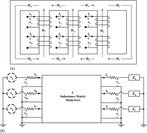
Time-domain techniques use analytical functions to model transformer primary and secondary circuits and core characteristics [17–25]. Saturation and hysteresis effects, as well as eddy-current losses, are included with acceptable degrees of accuracy. These techniques are mostly used for the electromagnetic transient analysis (such as inrush currents, overvoltages, geomagnetically induced currents, and out-of-phase synchronization) of multiphase and multilimb core-type power transformers under (un)balanced (non)sinusoidal excitations with (non)linear loads. The main limitation of time-domain techniques is the relatively long computing time required to solve the set of differential equations representing transformer dynamic behavior. They are not usually used for steady-state analyses. Harmonic modeling of power transformers in the time domain are performed by some popular software packages and circuit simulators such as EMTP [24] and DSPICE (Daisy’s version of circuit simulator SPICE [25]). The electromagnetic mathematical model of multiphase, multilimb core-type transformer is obtained by combining its electric and the magnetic circuits [35–37]. The principle of duality is usually applied to simplify the magnetic circuit. Figure 2.22 illustrates the topology and the electric equivalent circuit for the general case of a five-limb transformer, from which other configurations such as three-phase, three-limb, and single-phase ones can be derived. The open ends of the nonlinear multiport inductance matrix L (or its inverse, the reluctance matrix ℜ) allow the connection for any electrical configuration of the source and the load at the terminals of the transformer.
Most time-domain techniques are based on a set of differential equations defining transformer electric and magnetic behaviors. Their computational effort involves the numerical integration of ordinary differential equations (ODEs), which is an iterative and time-consuming process. Other techniques use Newton methodology to accelerate the solution [22,23]. Transformer currents and/or flux linkages are usually selected as variables. Difficulties arise in the computation and upgrading of magnetic variables (e.g., flux linkages), which requires the solution of the magnetic circuit or application of the nonlinear hysteresis characteristics, as discussed in Section 2.4.2.
In the next section, time-domain modeling based on state-space formulation of transformer variables is explained. Either transformer currents and/or flux linkages may be used as the state variables. Some models [22,23] prefer flux linkages since they change more slowly than currents and more computational stability is achieved.
2.4.3.1 State-Space Formulation
The state equation for an m-phase, n-winding transformer in vector form is [19]

where ![]() ,
, ![]() ,
, ![]() ,
, ![]() , and
, and ![]() are the terminal voltage vector, the current vector, the resistance matrix, the leakage inductance matrix, and the flux linkage vector, respectively.
are the terminal voltage vector, the current vector, the resistance matrix, the leakage inductance matrix, and the flux linkage vector, respectively.
The flux linkage vector can be expressed in terms of the core flux vector by

where ![]() is the transformation ratio matrix (number of turns) and
is the transformation ratio matrix (number of turns) and ![]() is the core-flux vector.
is the core-flux vector.
In general, the core fluxes are nonlinear functions of the magnetomotive forces (![]() ), therefore,
), therefore, ![]() can be expressed as
can be expressed as

where ![]() is a m × m Jacobian matrix. The magnetomotive force vector can be expressed in terms of the terminal current vector by
is a m × m Jacobian matrix. The magnetomotive force vector can be expressed in terms of the terminal current vector by
where ![]() is a matrix that can be determined from matrix
is a matrix that can be determined from matrix ![]() and the configuration of the transformer.
and the configuration of the transformer.
Substituting Eqs. 2-42 and 2-43 into Eq. 2-40, we obtain

Defining the nonlinear incremental (core) inductance

the transformer state equation is finally expressed as follows:

Equations 2-45 and 2-46 are the starting point for all modeling techniques based on the decoupling of magnetic and electric circuits. The basic difficulty is the calculation of the elements of the Jacobian ![]() at each integration step. The incorporation of nonlinear effects (such as magnetic saturation and hysteresis) and the computation of
at each integration step. The incorporation of nonlinear effects (such as magnetic saturation and hysteresis) and the computation of ![]() are performed by appropriate modifications of the differential and algebraic equations (Eqs. 2-40 to 2-46). As discussed in Section 2.4.2, numerous possibilities are available for accurate representation of transformer saturation and hysteresis. However, there is a trade-off between accuracy and computational speed of the solution. Figure 2.23 shows the flowchart of the nonlinear iterative algorithm for transformer modeling based on Eqs. 2-40 to 2-46, where elements of
are performed by appropriate modifications of the differential and algebraic equations (Eqs. 2-40 to 2-46). As discussed in Section 2.4.2, numerous possibilities are available for accurate representation of transformer saturation and hysteresis. However, there is a trade-off between accuracy and computational speed of the solution. Figure 2.23 shows the flowchart of the nonlinear iterative algorithm for transformer modeling based on Eqs. 2-40 to 2-46, where elements of ![]() can be derived from the solution of transformer magnetic circuit with a piecewise linear (Fig. 2.16b) or an incremental (Fig. 2.16c) magnetizing characteristic [19].
can be derived from the solution of transformer magnetic circuit with a piecewise linear (Fig. 2.16b) or an incremental (Fig. 2.16c) magnetizing characteristic [19].

2.4.3.2 Transformer Steady-State Solution from the Time-Domain Simulation
Conventional time-domain transformer models based on the brute force (BF) procedure [22,23] are not usually used for the computation of the periodic steady-state solution because of the computational effort involved requiring the numerical integration of ODEs until the initial transient decays. This drawback is overcome with the introduction of numerical differentiation (ND) and Newton techniques to enhance the acceleration of convergence [22,23].
2.4.4 Frequency-Domain Simulation of Power Transformers
Frequency- or harmonic-domain simulation techniques use Fourier analysis to model the transformer’s primary and secondary parameters and to approximate core nonlinearities [26–29]. Most frequency-based models ignore hysteresis and eddy currents or use some measures (e.g., the concept of describing functions as discussed in Section 2.4.2.5) to approximate them; therefore, they are not usually as accurate as time-domain models. Harmonic-based simulation techniques are relatively fast, which makes them fine candidates for steady-state analysis of power transformers. Most (but not all) frequency-domain analyses assume balanced three-phase operating conditions and single-limb transformers (bank of single-phase transformers).
Figure 2.24 shows a frequency-domain transformer model in the form of the harmonic Norton equivalent circuit. Standard frequency-domain analyses are used to formulate the transformer’s electric circuits whereas frequency-based simulation techniques are required to model magnetic circuits. Figure 2.25 shows the flowchart of the nonlinear iterative algorithm for transformer modeling in the frequency domain. At each step of the algorithm, harmonic current sources Ĩcore(h) and Ĩmag(h) are upgraded using a frequency-based model for the transformer core, as discussed in Sections 2.4.2.4 and 2.4.2.5. Some references use the harmonic lattice representation of multilimb, three-phase transformers to define a harmonic Norton equivalent circuit [27]. The main limitations of this approach, as with all frequency-based simulation techniques, are the approximations used for modeling transformer magnetic circuits.


2.4.5 Combined Frequency- and Time-Domain Simulation of Power Transformers
To overcome the limitations of frequency-based techniques and to preserve the advantages of the time-domain simulation, most transformer models use a combination of frequency-domain (to model harmonic propagation on primary and secondary sides) and time-domain (to model core nonlinearities) analyses to achieve the steady-state solution with acceptable accuracy and speed [30,31,1–4]. Thus, accurate modeling of saturation, hysteresis, and eddy-current phenomena are possible. Combined frequency- and time-domain models are fine candidates for steady-state analysis of power transformers. Figure 2.26 shows the flowchart of the nonlinear iterative algorithm for transformer modeling in the frequency and time domains. Transformer electric circuits are models for standard frequency-domain techniques whereas the magnetic analysis is accurately performed in the time domain. At each step of the algorithm, instantaneous flux linkages (λ(t)) and transformer (λ - i) characteristics are used to compute the instantaneous magnetizing (imag(t)) and core-loss (icore(t)) currents, as discussed in Sections 2.4.2.1 to 2.4.2.4. Fast Fourier transformation (FFT) is performed to compute and upgrade harmonic current sources Ĩcore(h) and Ĩmag(h).

2.4.6 Numerical (Finite-Difference, Finite-Element) Simulation of Power Transformers
These accurate and timely simulation techniques are based on two- or three-dimensional modeling of the anisotropic power transformer [1–4, 6, 32–34]. They require detailed information about transformer size, structure, and materials. The anisotropic transformer’s magnetic core is divided into small (two- or three-dimensional) meshes or volume elements, respectively. Within each mesh (element), isotropic materials and linear B–H characteristics are assumed. The resulting linear equations are solved using matrix solution techniques. Mesh equations are related to each other by boundary conditions. With these nonlinear and time-consuming techniques, simultaneous consideration of most transformer nonlinearities are possible. Finite element/difference techniques are the most accurate tools for transformer modeling under sinusoidal and nonsinusoidal operating conditions. Numerical (e.g., finite-element and finite-difference) software packages are available for the simulation of electromagnetic phenomena. However, numerical techniques are not very popular since they require much detailed information about transformer size, air gaps, and materials that makes their application a tedious and time-consuming process.
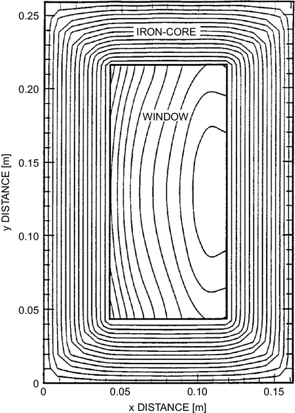
Figure 2.27 illustrates the construction of a single-phase 25 kVA pole transformer as it is widely employed in residential single-phase systems. The butt-to-butt air gaps and the interlamination gaps of the wound core of Fig. 2.27 are illustrated in Fig. 2.28. These air gaps, grain orientation of the electrical steel (anisotropy), and saturation of the iron core require the calculation of representative reluctivities as indicated in Fig. 2.29. These representative reluctivity data are used for the computation of the end-region (y–z plane) and x–y planes of the single-phase transformer as depicted in Figs. 2.30 and 2.31, respectively. Measured and computed flux-linkage versus current characteristics are presented in Fig. 2.32. Detailed analyses are given in references [1–4] and [36].


2.5 Ferroresonance of power transformers
Before discussing ferroresonance phenomena, it may be good to review resonance as it occurs in a linear RLC circuit, as shown in Fig. 2.33. The current is


From the above equation we observe that whenever the value of the capacitive reactance XC equals the value of the inductive reactance XL, the current in the circuit only is limited by the resistance R. Very often the value of R can be very small compared with XL or XC, in which case the current can reach very high levels (resonant current).
Now let us look at a simple power circuit, consisting of a transformer connected to a power system as shown by Fig. 2.34; its single-phase equivalent circuit is illustrated in Fig. 2.35. Even though switch S2 is open, a current i(t) can still flow because the cable shunt capacitance C closes the circuit. The transformer is assumed to be unloaded but energized. The magnetizing current i(t) has to return to its source via the cable shunt capacitance C. Therefore, Resonance occurs whenever XL and XC are close to each other.


In power systems, the variations of XL are mainly due to the nonlinear magnetizing inductance of transformers, as shown in Fig. 2.36, and most changes in XC are caused by switching capacitor banks and cables. The capacitance between two charged plates is illustrated in Fig. 2.37.


2.5.1 System Conditions Susceptible (Contributive, Conducive) to Ferroresonance
In the previous section, a single-phase circuit was used to explain in a simplified manner the problem of ferroresonance. Here, three-phase systems will be covered because they are the basic building block of a power system and, as will be shown, they are the most prone to this problem.
Now that the principle of ferroresonance has been explained, the next important question is what conditions in an actual power system are contributive (conducive) to ferroresonance? Some conditions may not by themselves initiate the problem, but they certainly are prerequisites (necessary) so that when other conditions are present in a power system, ferroresonance can occur. The purpose of the next section is to prevent these prerequisite conditions.
2.5.2 Transformer Connections and Single-Phase (Pole) Switching at No-Load
The transformer is the basic building block in stepping up or down voltages and currents in a power system. It is also one of the basic elements of a ferroresonant circuit. The two most widely used transformer connections are the wye and delta. Each one has its advantages and disadvantages, and depending on the particular application and engineering philosophies, one or the other or a combination of both will be used. First we will look at the delta connected (at primary) transformer, as shown in Fig. 2.38. Figure 2.38a shows a simple power system. The source of power is represented by a grounded equivalent power source because normally the system is grounded at the source and/or at some other points in the power system. The connection between the source and the transformer is made by an (underground) cable having a capacitance C.


There are four prerequisites for ferroresonance:
• The first prerequisite for ferroresonance is the employment of cables with relatively large capacitances. The transformer primary is delta connected or in ungrounded wye connection, while the secondary can be either grounded or ungrounded wye or delta connected. This system is shown in Fig. 2.38a and the transformer is assumed to be unloaded (load provides damping).
• The second prerequisite for ferroresonance is the transformer connection.
• The third prerequisite for ferroresonance is an unloaded transformer. In order to simplify this discussion, the coupling capacitances of the transformer (from phase to ground, phase to phase, and from primary to secondary) will be assumed to be low enough compared with the shunt capacitance of the primary line (cables in populated areas) so that they can be neglected. However, it must be noted that at voltage levels above 15 kV the coupling capacitances (increased insulation) of the transformer become more important so that their contribution to the ferroresonant circuit cannot be neglected.
• The fourth prerequisite is when either one or two phases are connected; then these circuit configurations are susceptible to ferroresonance. When the third phase is energized, the system will be balanced and the current will flow directly to and from the transformer, bypassing the capacitance to ground.
Adding a load to the secondary side of the transformer changes the ferroresonant circuit considerably: the effective load impedance ZL will be reflected back into the primary side by the square of the turns ratio of the primary (N1) to the secondary (N2). This reflected impedance ![]() will in turn limit considerably the current in the ferroresonant circuit, thus reducing the possibility of this phenomenon significantly.
will in turn limit considerably the current in the ferroresonant circuit, thus reducing the possibility of this phenomenon significantly.
Now let us look at a transformer with its primary winding connected ungrounded wye as shown in Fig. 2.39. Note that the source is shown grounded and that the unloaded secondary side of the transformer can be connected either ungrounded wye or delta. When one (or two) phase(s) is (are) energized, a closed loop is formed, consisting of transformer windings and the capacitance of the primary conductor (cable) to ground. The resulting large nonsinusoidal magnetizing current can induce ferroresonant overvoltages in the circuit generating large losses within the transformer. As in the previous case, a secondary load can greatly reduce the probability of ferroresonance.


A single-phase transformer connected phase-to-phase to a grounded supply is also likely to become ferroresonant when one of the phases is opened or closed, as shown in Fig. 2.40. If on the other hand, the transformer is connected phase to ground to a grounded source (Fig. 2.41), the circuit is not likely to become ferroresonant when the hot line (S1) is opened.


The mere presence of the ferroresonant circuit does not necessarily mean that the circuit involved will experience overvoltages due to this problem. The ratio of the capacitive reactance XC to the transformer magnetizing reactance Xt of the ferroresonant circuit (XC/Xt) will determine whether the circuit will experience overvoltages or not. These tests have been generalized to cover a wide range of transformer sizes (15 kVA to 15 MVA) and line-to-ground (line-to-neutral) voltages ranging from 2.5 to 19.9 kV, and it has been determined that for three-phase core type banks, they will experience overvoltages above 1.1–1.25 pu when the ratio XC/Xt < 40, where Xt = ωL, XC = 1/ωC or ![]() . Note that a three-limb, three-phase transformer has a smaller zero-sequence reactance than that of a bank of three single-phase transformers or that of a five-limb, three-phase transformer [38–41].
. Note that a three-limb, three-phase transformer has a smaller zero-sequence reactance than that of a bank of three single-phase transformers or that of a five-limb, three-phase transformer [38–41].
For banks of single-phase transformers, a ratio XC/Xt < 25 has been found to produce overvoltages when the ferroresonant circuit is present.
2.5.2.1 Application Example 2.6: Susceptibility of Transformers to Ferroresonance
Assuming linear (λ - i) characteristics with λ = 0.63 Wb-turns at 0.5 A, we have


Therefore, XC/Xt = 0.055 < 40, that is, ferroresonance is likely to occur.
2.5.3 Ways to Avoid Ferroresonance
Now that the factors conducive to ferroresonance have been identified, the next question is how to avoid the problem or at least try to mitigate its effects as much as possible. There are a few techniques to limit the probability of ferroresonance:
• The grounded-wye/grounded-wye transformer. When the neutral of the transformer is grounded, the capacitance to ground of the line (cable) is essentially bypassed, thus eliminating the series LC circuit that can initiate ferroresonance. It is recommended that the neutral of the transformer be solidly grounded to avoid instability in the neutral of the transformer (grounding could be done indirectly via a “Peterson coil” to limit short-circuit currents). When the neutral of a wye/wye transformer is grounded, other things can happen too: if the grounded three-phase bank is not loaded equally on its three phases, the currents flowing in the bank and consequently the fluxes will not cancel out to zero. If the bank is a three-limb core transformer, the resultant flux will be forced to flow outside the core. Under these conditions, this flux will be forced to flow in the tank of the transformer, thus causing a current to circulate in it, which can cause excessive tank overheating if the imbalance is large enough. Another approach is to use banks made up of three single-phase units or three-phase, five-limb core transformers. When single-phase units are used, the flux for each phase will be restricted to its respective core. In the case of the five-limb core, the two extra limbs provide the path for the remaining flux due to imbalance.
• Limiting the cable capacitance by limiting the length of the cable. This is not a practical technique.
• Fast three-phase switching to avoid longer one- and two-phase connections. This is an effective but expensive approach
• Use of cables with low capacitance [42–44].
2.5.3.1 Application Example 2.7: Calculation of Ferroresonant Currents within Transformers
The objective of this example is to study the (chaotic) phenomenon of ferroresonance in transformers using Mathematica or MATLAB.
Consider a ferroresonant circuit consisting of a sinusoidal voltage source v(t), a (cable) capacitance C, and a nonlinear (magnetizing) impedance (consisting of a resistance R and an inductance L) connected in series, as shown in Fig. E2.7.1. If the saturation curve (flux linkages λ as a function of current i) is represented by the cubic function i = aλ3, the following set of first-order nonlinear differential equations can be formulated:

or in an equivalent manner, one can formulate the second-order nonlinear differential equation

where k = 3aR, b = Vmaxω, and C = a.
a) Show that the above equations are true for the circuit of Fig. E2.7.1.
b) The system of Fig. E2.7.1 displays for certain values of the parameters b = Vmaxω and k = 3aR (ω = 2πf where f = 60 Hz, R = 0.1 Ω, C = 100 μF, a = C, low voltage ![]() , and high voltage
, and high voltage ![]() ), which characterize the source voltage and the resistive losses of the circuit, respectively, chaotic behavior as described by [45]. For zero initial conditions –using Mathematica or MATLAB – compute numerically λ, dλ/dt, and i as a function of time from tstart = 0 to tend = 0.5 s.
), which characterize the source voltage and the resistive losses of the circuit, respectively, chaotic behavior as described by [45]. For zero initial conditions –using Mathematica or MATLAB – compute numerically λ, dλ/dt, and i as a function of time from tstart = 0 to tend = 0.5 s.
c) Plot λ versus dλ/dt for the values as given in part b.
d) Plot λ and dλ/dt as a function of time for the values as given in part b.
e) Plot i as a function of time for the values as given in part b.
f) Plot voltage dλ/dt versus i for the values as given in part b.

Solution to Application Example 2.7
a) To show that the equations are true use the circuit of Fig. E2.7.1:
By inspection of the circuit of Figure E2.7.1:


Taking the derivative of the circuit equation:

For k = 3aR, b = ωVmax, and C = a,

b) To compute numerical values of λ, dλ/dt, and i as a function of time for 0 < t < 0.5 s (f = 60 Hz, R = 0.1 Ω, C = a = 100 μF, ![]() , all initial conditions = 0) use the MATLAB codes of Table E2.7.1.
, all initial conditions = 0) use the MATLAB codes of Table E2.7.1.
Table E2.7.1
MATLAB Program Codes for Application Example 2.7
|
% Matlab code % % getting started clear all; close all; nfig = 0; % % define integration variables and initial % conditions to = 0; tf = 0.5; % time in seconds xo = 0; vo = 0; % initial conditions zo = [xo vo]′ ; % initial conditions in vector form %Vmax = [1000*sqrt(2):100:20000*sqrt(2)]; %Vmax = 20000*sqrt(2); %b = 2*pi*60*Vmax; %w = 2*pi*60; %k = 3*100e-6*0.1; % Evaluate z numerically [t, z] = ode23(‘Hw5eqnfile’, [to tf], zo); %x = dsolve(‘D2x+k*xˆ2*Dx+xˆ3=b*cos(w*t)’, % ‘x(0)=0’); %y = rk2(‘D2y+k*yˆ2*Dy+yˆ3=b*cos(w*t)’, [00.5], [0 0 0]) %dxdt = [x(2); b*cos(w*t)-Dx(2)-k*x(1)ˆ2*x(2)-x(1)ˆ3]; % % Evaluate x(t) analytically % te = linspace (to, tf, 200); % xe = 0.7737*exp(-3*te). *cos(2*te-1.1903) - 0.3095*cos(5*te-0.3805); % % Plot profiles nfig = nfig+1; figure (nfig) plot (t, z(:, 1)), grid xlabel (‘Time (s)’), ylabel (‘Inductor Flux Linkage’) nfig = nfig+1; figure (nfig) plot (t,z (:, 2)), grid xlabel (‘Time (s)’), ylabel (‘Voltage’) nfig = nfig+1; figure (nfig) plot(t, 100e-6*z(:,1).ˆ3), grid xlabel(‘Time (s)’), ylabel (‘Current’) % Plot dx/dt versus x(t) nfig = nfig+1; figure (nfig) plot (z(:, 2), z(:,1), zo(1), zo(2), ‘rx’), grid xlabel (‘Voltage’), ylabel (‘Inductor Flux Linkage’) % Plot dx/dt versus i(t) nfig = nfig+1; figure (nfig) plot (100e-6*z(:, 1).ˆ3, z(:,2), zo(1), zo(2), ‘rx’), grid xlabel(‘Current’), ylabel (‘Voltage’) |

c) Plots of λ versus dλ/dt for the values as given in part b are shown in Figs. E2.7.2 and E2.7.3.

 .
.
 .
.d) Plots of λ and dλ/dt as a function of time for the values given in part b are shown in Figs. E2.7.4 through E2.7.7.

 .
.
 .
.
 .
.
 .
.e) Plots of i as a function of time for the values as given in part b are shown in Figs. E2.7.8 and E2.7.9.

 .
.
 .
.f) Plots of voltage v = dλ/dt versus i for the values as given in part b are shown in Figs. E2.7.10 and E2.7.11.

 .
.
 .
.2.6 Effects of solar-geomagnetic disturbances on power systems and transformers
Solar flares and other solar phenomena can cause transient fluctuations in the earth’s magnetic field (e.g., Bearth = 0.6 gauss = 60 μT). When these fluctuations are severe, they are known as geomagnetic storms and are evident visually as the aurora borealis in the Northern Hemisphere and as the aurora australis in the Southern Hemisphere (Fig. 2.42).

These geomagnetic field changes induce an earth-surface potential (ESP) that causes geomagnetically induced currents (GICs) to flow in large-scale 50 or 60 Hz electric power systems. The GICs enter and exit the power system through the grounded neutrals of wye-connected transformers that are located at opposite ends of a long transmission line. The causes and nature of geomagnetic storms and their resulting effects in electric power systems will be described next.
2.6.1 Application Example 2.8: Calculation of Magnetic Field Strength 
The magnetic field strength ![]() of a wire carrying 100 A at a distance of R = 1 m (Fig. E2.8.1) is
of a wire carrying 100 A at a distance of R = 1 m (Fig. E2.8.1) is
or

 field of a single conductor in free space.
2.6.2 Solar Origins of Geomagnetic Storms
The solar wind is a plasma of protons and electrons emitted from the sun due to
• coronal holes, and
• disappearing filaments.
The solar wind particles interact with the earth’s magnetic field in a complicated manner to produce auroral currents that follow circular paths (see Fig. 2.42) around the geomagnetic poles at altitudes of 100 km or more. These auroral currents produce fluctuations in the earth’s magnetic field (ΔB = ± 500 nT = ± 0.5 μT) that are termed geomagnetic storms when they are of sufficient severity.
2.6.3 Sunspot Cycles and Geomagnetic-Disturbance Cycles
On average, solar activity as measured by monthly sun spot numbers follows an 11-year cycle [46–53]. The last sunspot cycle 23 had its minimum in September 1997, and its peak in 2001–2002. The largest geomagnetic storms are most likely due to flare and filament eruption events and could occur at any time during the cycle; the severe geomagnetic storm on March 13, 1989 (Hydro Quebec system collapsed with 21.5 GW) was evidently a striking example.
2.6.4 Earth-Surface Potential (ESP) and Geomagnetically Induced Current (GIC)
The auroral currents that result from solar-emitted particles interact with the earth’s magnetic field and produce fluctuations in the earth’s magnetic field Bearth. The earth is a conducting sphere, admittedly nonhomogeneous, that experiences (or at least portions of it) a time-varying magnetic field. The portions of the earth that are exposed to the time-varying magnetic field will have electric potential gradients (voltages) induced, which are termed earth-surface potentials (ESPs). Analytical methods have been developed to estimate the ESP based on geomagnetic field fluctuation data and a multilayered earth conductivity model: values in the range of 1.2–6 V/km or 2–10 V/mile can be obtained during severe geomagnetic storms in regions of low earth conductivity. Low earth conductivity (high resistivity) occurs in regions of igneous rock geology (e.g., Rocky Mountain region). Thus, power systems located in regions of igneous rocky geology are the most susceptible to geomagnetic storm effects.
Electric power systems become exposed to the ESP through the grounded neutrals of wye-connected transformers that may be at the opposite ends of long transmission lines. The ESP acts eventually as an ideal voltage source impressed across the grounded-neutral points and because the ESP has a frequency of one to a few millihertz, the resulting GICs can be determined by dividing the ESP by the equivalent DC resistance of the paralleled transformer winding and line conductors between the two neutral grounding points. The GIC is a quasi-direct current, compared to 50 or 60 Hz, and GIC values in excess of 100 A have been measured in transformer neutrals [46–53].
Ampere’s law is valid for the calculation of the aurora currents of Fig. 2.42

2.6.5 Power System Effects of GIC
GIC must enter and exit power systems through the grounded-neutral connections of wye-connected transformers or autotransformers. The per-phase GIC can be many times larger in magnitude than the rms AC magnetizing current of a transformer. The net result is a DC bias in the transformer core flux, resulting in a high level of half-cycle saturation [40,54]. This half-cycle saturation of transformers operating within a power system is the source of nearly all operating and equipment problems caused by GICs during magnetic storms (reactive power demand and its associated voltage drop). The direct consequences of the half-cycle transformer saturation are
• The transformer becomes a rich source of even and odd harmonics;
• A great increase in inductive power (VAr) drawn by the transformer occurs resulting in an excessive voltage drop; and
• Large stray leakage flux effects occur with resulting excessive localized (e.g., tank) heating.
There are a number of effects due to the generation of high levels of harmonics by system power transformers, including
• overheating of capacitor banks,
• possible misoperation of relays,
• sustained overvoltages on long-line energization,
• higher secondary arc currents during single-pole switching,
• higher circuit breaker recovery voltage,
• overloading of harmonic filters of high voltage DC (HVDC) converter terminals, and
• distortion of the AC voltage wave shape that may result in loss of power transmission.
The increased inductive VArs drawn by system transformers during half-cycle saturation are sufficient to cause intolerable system voltage depression, unusual swings in MW and MVAr flow on transmission lines, and problems with generator VAr limits on some instances.
2.6.6 System Model for Calculation of GIC
The ESP and GIC due to geomagnetic storms have frequencies in the millihertz range, and appear as quasi-DC in comparison to 50 and 60 Hz power system frequencies. Thus the system model is basically a DC conducting path model, in which the ESP voltage sources, in series with station ground-mat resistances, transformer resistances, and transmission line resistances, are impressed between the neutral grounds of all grounded-wye transformers.
Although there are similarities between the paths followed by GIC and zero-sequence currents in a power system, there are also important differences in the connective topography representing transformers in the two instances. The GIC transformer models are not concerned with leakage reactance values, but only with paths through the transformer that could be followed by DC current. Thus, the zero-sequence network configuration of an AC transmission line grid cannot be used directly to determine GIC. Transmission lines can be modeled for GIC determination by using their positive-sequence resistance values with a small correction factor to account for the differences between AC and DC resistances due to skin, proximity, and magnetic loss effects. A simple three-phase network is shown in Fig. 2.43, and the DC equivalent for determining GIC is shown by Fig. 2.44 [46–54]. The symbols used are defined as follows:


RL ≡ line resistance per phase,
RY ≡ resistance of grounded wye-connected winding per phase,
RS ≡ autotransformer series winding resistance per phase,
RC ≡ autotransformer common winding resistance per phase,
Rgi ≡ grounding resistance of bus i,
Ini ≡ neutral GIC at bus i, and
VESPi ≡ earth surface potential at bus i.
2.6.7 Mitigation Techniques for GIC
Much work has been done [46–54] after some power system failures have occurred during the past 20 years. The most important finding is that three-limb, three-phase transformers with small zero-sequence reactances – requiring a relatively large air gap between iron core and solid iron tank – are least affected by geomagnetically induced currents.
2.6.8 Conclusions Regarding GIC
Geomagnetic storms are naturally occurring phenomena that can adversely affect electric power systems. Only severe storms produce power system effects. Power systems in northern latitudes that are in regions of high geological resistivity (igneous rock formations) are more susceptible. Three limb, three-phase transformers with large gaps between iron core and tank permit GICs to flow but suppress their detrimental effects such as VAr demand [39,46–54]. The mitigation techniques of Section 2.6.7 have been implemented and for this reason now a major collapse of power systems due to geomagnetic storms can be avoided. This is an example of how research can help increase the reliability of power systems.