1.8.1 High Power Quality Equipment Design

The use of nonlinear and electronic-based devices is steadily increasing and it is estimated that they will constitute more than 70% of power system loading by year 2010 [10]. Therefore, demand is increasing for the designers and product manufacturers to produce devices that generate lower current distortion, and for end users to select and purchase high power quality devices. These actions have already been started in many countries, as reflected by improvements in fluorescent lamp ballasts, inclusion of filters with energy saving lamps, improved PWM adjustable-speed drive controls, high power quality battery chargers, switch-mode power supplies, and uninterruptible power sources.

1.8.2 Harmonic Cancellation

There are some relatively simple techniques that use transformer connections to employ phase-shifting for the purpose of harmonic cancellation, including [10]:

• delta-delta and delta-wye transformers (or multiple phase-shifting transformers) for supplying harmonic producing loads in parallel (resulting in twelve-pulse rectifiers) to eliminate the 5th and 7th harmonic components,

• transformers with delta connections to trap and prevent triplen (zero-sequence) harmonics from entering power systems,

• transformers with zigzag connections for cancellation of certain harmonics and to compensate load imbalances,

• other phase-shifting techniques to cancel higher harmonic orders, if required, and

• canceling effects due to diversity [57–59] have been discovered.

1.8.3 Dedicated Line or Transformer

Dedicated (isolated) lines or transformers are used to attenuate both low- and high-frequency electrical noise and transients as they attempt to pass from one bus to another. Therefore, disturbances are prevented from reaching sensitive loads and any load-generated noise and transients are kept from reaching the remainder of the power system. However, some common-mode and differential noise can still reach the load. Dedicated transformers with (single or multiple) electrostatic shields are effective in eliminating common-mode noise.

Interharmonics (e.g., caused by induction motor drives) and voltage notching (e.g., due to power electronic switching) are two examples of problems that can be reduced at the terminals of a sensitive load by a dedicated transformer. They can also attenuate capacitor switching and lightning transients coming from the utility system and prevent nuisance tripping of adjustable-speed drives and other equipment. Isolated transformers do not totally eliminate voltage sags or swells. However, due to the inherent large impedance, their presence between PCC and the source of disturbance (e.g., system fault) will lead to relatively shallow sags.

An additional advantage of dedicated transformers is that they allow the user to define a new ground reference that will limit neutral-to-ground voltages at sensitive equipment.

1.8.3.1 Application Example 1.6: Interharmonic Reduction by Dedicated Transformer

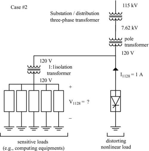
Figure E1.6.1 shows a typical distribution system with linear and nonlinear loads. The nonlinear load (labeled as “distorting nonlinear load”) consists of two squirrel-cage induction motors used as prime movers for chiller-compressors for a building’s air-conditioning system. Note the thyristor symbol represents the induction motors, although there are no thyristors present: the thyristor symbol represents here a nonlinearity. This load produces interharmonic currents that generate interharmonic voltage drops across the system’s impedances resulting in the interharmonic content of the line-to-line voltage of the induction motors as given by Table E1.6.1. Some of the loads are very sensitive to interharmonics and these must be reduced at the terminals of sensitive loads. These loads are labeled as “sensitive loads.”

Table E1.6.1

Interharmonics of Phase Current and Line-to-Line Voltage Generated by a Three-Phase Induction Motor [34]

Interharmonic fh (Hz)	Interharmonic amplitude of phase current (%)	Interharmonic amplitude of line-to-line voltage (%)
1128	7	0.40
1607	10	0.40
1730	10	0.55

Three case studies are considered:

• Case #1: Distorting nonlinear load and sensitive loads are fed from the same pole transformer (Fig. E1.6.2).

• Case #2: A dedicated 1:1 isolation transformer is used between the distorting nonlinear load and sensitive loads (Fig. E1.6.3).

• Case #3: A dedicated 7.62 kV to 120 V pole transformer is used between the distorting nonlinear load and sensitive loads (Fig. E1.6.4).

Solution to Application Example 1.6

Computations are shown in Figs. E1.6.5 and E1.6.6 for the above three cases. As illustrated, for V_load1 = V_load2 the 1128th interharmonic amplitude is V₁₁₂₈ = $\frac{\left(122.64-120\right)}{120}$ (100%) = 2.2%, whereas for V_load3 this interharmonic is only 0.006%. This demonstrates the effectiveness of a dedicated line or transformer, other than an isolation transformer with a turns ratio 1 : 1.

1.8.4 Optimal Placement and Sizing of Capacitor Banks

It is well known that proper placement and sizing of shunt capacitor banks in distorted networks can result in reactive power compensation, improved voltage regulation, power factor correction, and power/energy loss reduction. The capacitor placement problem consists of determining the optimal numbers, types, locations, and sizes of capacitor banks such that minimum yearly cost due to peak power/energy losses and cost of capacitors is achieved, while the operational constraints are maintained within required limits.

Most of the reported techniques for capacitor placement assume sinusoidal operating conditions. These methods include nonlinear programming, and near global methods (genetic algorithms, simulated annealing, tabu search, artificial neural networks, and fuzzy theory). All these approaches ignore the presence of voltage and current harmonics [60,61].

Optimal capacitor bank placement is a well-researched subject. However, limited attention is given to this problem in the presence of voltage and current harmonics. Some publications have taken into account the presence of distorted voltages for solving the capacitor placement problem. These investigations include exhaustive search, local variations, mixed integer and nonlinear programming, heuristic methods for simultaneous capacitor and filter placement, maximum sensitivities selection, fuzzy theory, and genetic algorithms.

According to newly developed investigations based on fuzzy and genetic algorithms [60,61], proper placement and sizing of capacitor banks in power systems with nonlinear loads can result in lower system losses, greater yearly benefits, better voltage profiles, and prevention of harmonic parallel resonances, as well as improved power quality. Simulation results for the standard 18-bus IEEE distorted distribution system show that proper placement and sizing of capacitor banks can limit voltage and current harmonics and decrease their THDs to the recommended levels of IEEE-519, without application of any dedicated high-order passive or active filters. For cases where the construction of new capacitor bank locations is not feasible, it is possible to perform the optimization process without defining any new locations. Therefore, reexamining capacitor bank sizes and locations before taking any major steps for power quality mitigation is highly recommended.

Detailed analyses for optimal sizing and placement of capacitor banks in the presence of harmonics and nonlinear loads are presented in Chapter 10.

1.8.5 Derating of Power System Devices

Power system components must be derated when supplying harmonic loads. Commercial buildings have drawn the most attention in recent years due to the increasing use of nonlinear loads. According to the IEEE dictionary, derating is defined as “the intentional reduction of stress/strength ratio (e.g., real or apparent power) in the application of an item (e.g., cables, transformer, electrical machines), usually for the purpose of reducing the occurrence of stress-related failure (e.g., reduction of lifetime due to increased temperature beyond rated temperature).” As discussed in Section 1.5, harmonic currents and voltages result in harmonic losses of magnetic devices, increasing their temperature rise [62]. This rise beyond the rated value results in a reduction of lifetime, as will be discussed in Chapter 6.

There are several techniques for determining the derating factors (functions) of appliances for non-sinusoidal operating conditions (as discussed in Chapter 2), including:

• from tables in standards and published research (e.g., ANSI/IEEE Std C57.110 [63] for transformer derating),

• from measured (or computed) losses,

• by determining the K-factor, and

• based on the F_HL-factor.

1.8.6 Harmonic Filters, APLCs, and UPQCs

One means of ensuring that harmonic currents of nonlinear components will not unduly interact with the remaining part of the power system is to place filters near or close to nonlinear loads. The main function of a filter is either to bypass harmonic currents, block them from entering the power system, or compensate them by locally supplying harmonic currents. Due to the lower impedance of the filter in comparison to the impedance of the system, harmonic currents will circulate between the load and the filter and do not affect the entire system; this is called series resonance. If other frequencies are to be controlled (e.g., that of arc furnaces), additional tuned filters are required.

Harmonic filters are broadly classified into passive, active, and hybrid structures. These filters can only compensate for harmonic currents and/or harmonic voltages at the installed bus and do not consider the power quality of other buses. New generations of active filters are active-power line conditioners that are capable of minimizing the power quality problems of the entire system.

Passive filters are made of passive components (inductance, capacitance, and resistance) tuned to the harmonic frequencies that are to be attenuated. The values of inductors and capacitors are selected to provide low impedance paths at the selected frequencies. Passive filters are generally designed to remove one or two harmonics (e.g., the 5th and 7th). They are relatively inexpensive compared with other means for eliminating harmonic distortion, but also suffer from some inherent limitations, including:

• Interactions with the power system;

• Forming parallel resonance circuits with system impedance (at fundamental and/or harmonic frequencies). This may result in a situation that is worse than the condition being corrected. It may also result in system or equipment failure;

• Changing characteristics (e.g., their notch frequency) due to filter parameter variations;

• Unsatisfactory performance under variations of nonlinear load parameters;

• Compensating a limited number of harmonics;

• Not considering the power quality of the entire system; and

• Creating parallel resonance. This resonance frequency must not necessarily coincide with any significant system harmonic. Passive filters are commonly tuned slightly lower than the attenuated harmonic to provide a margin of safety in case there are some changes in system parameters (due to temperature variations and/or failures). For this reason filters are added to the system starting with the lowest undesired harmonic. For example, installing a seventh-harmonic filter usually requires that a fifth-harmonic filter also be installed.

Designing passive filters is a relatively simple but tedious matter. For the proper tuning of passive filters, the following steps should be followed:

• Model the power system (including nonlinear loads) to indicate the location of harmonic sources and the orders of the injected harmonics. A harmonic power (load) flow algorithm (Chapter 7) should be used; however, for most applications with a single dominating harmonic source, a simplified equivalent model and hand calculations are adequate;

• Place the hypothetical harmonic filter(s) in the model and reexamine the system. Filter(s) should be properly tuned to dominant harmonic frequencies; and

• If unacceptable results (e.g., parallel resonance within system) are obtained, change filter location(s) and modify parameter values until results are satisfactory.

In addition to power quality improvement, harmonic filters can be configured to provide power factor correction. For such cases, the filter is designed to carry resonance harmonic currents, as well as fundamental current.

Active filters rely on active power conditioning to compensate for undesirable harmonic currents. They actually replace the portion of the sine wave that is missing in the nonlinear load current by detecting the distorted current and using power electronic switching devices to inject harmonic currents with complimentary magnitudes, frequencies, and phase shifts into the power system. Their main advantage over passive filters is their fine response to changing loads and harmonic variations. Active filters can be used in very difficult circumstances where passive filters cannot operate successfully because of parallel resonance within the system. They can also take care of more than one harmonic at a time and improve or mitigate other power quality problems such as flicker. They are particularly useful for large, distorting nonlinear loads fed from relatively weak points of the power system where the system impedance is relatively large. Active filters are relatively expensive and not feasible for small facilities.

Power quality improvement using filters, unified power quality conditioners (UPQCs), and optimal placement and sizing of shunt capacitors, are discussed in Chapters 9 and 10, respectively.

1.8.6.1 Application Example 1.7: Hand Calculation of Harmonics Produced by Twelve-Pulse Converters

Figure E1.7.1 shows a large industrial plant such as an oil refinery or chemical plant [64] being serviced from a utility with transmission line-to-line voltage of 115 kV. The demand on the utility system is 50 MVA and 50% of its load is a twelve-pulse static power converter load.

Table E1.7.1 lists the harmonic currents (I_h) given in pu of the fundamental current based on the commutating reactance X_c^h = 0.12 pu and the firing angle α = 30° of six-pulse and twelve-pulse converters. In an ideal twelve-pulse converter, the magnitude of some current harmonics (bold in Table E1.7.1) is zero. However, for actual twelve-pulse converters, the magnitudes of these harmonics are normally taken as 10% of the six-pulse values [64]. Assume ${\left.R_{SC}\right|}_{PCC\#1}=40$ pu, and ${\left.R_{SC}\right|}_{PCC\#2}=8.7$ pu.

Table E1.7.1

Harmonic Current (I_h) Generated by Six-Pulse and Twelve-Pulse Converters [64] Based on $X_c^h=0.12\mathrm{p}\mathrm{u}$ and α = 30°

Harmonic order (h)	Ih for 6-pulse converter (pu)	Ih for 12-pulse converter (pu)
1	1.000	1.000
5	0.192	0.0192
7	0.132	0.0132
11	0.073	0.073
13	0.057	0.057
17	0.035	0.0035
19	0.027	0.0027
23	0.020	0.020
25	0.016	0.016
29	0.014	0.0014
31	0.012	0.0012
35	0.011	0.011
37	0.010	0.010
41	0.009	0.0009
43	0.008	0.0008
47	0.008	0.008
49	0.007	0.007

Solution to Application Example 1.7

1.8.6.2 Application Example 1.8: Filter Design to Meet IEEE-519 Requirements

Filter design for Application Example 1.7 will be performed to meet the IEEE-519 requirements. The circuit of Fig. E1.7.1 is now augmented with a passive filter, as shown by Fig. E1.8.1.

Solution to Application Example 1.8

System Analysis

At harmonic frequencies, the circuit of Fig. E1.8.1 can be approximated by the equivalent circuit shown by Fig. E1.8.2. This circuit should be analyzed at each frequency of interest by calculating series and parallel resonances.

For series resonance Ĩ_fh is large whereas for parallel resonance Ĩ_fh and Ĩ_sysh are large. The major impedance elements in the circuit respond differently as frequency changes. The impedance of the transmission line Z_lineh is a complicated relationship between the inductive and capacitive reactances. Using the fundamental frequency resistance R and inductance of the transmission line, however, gives acceptable results. For most industrial systems Z_th and Z_lineh can be approximated by the short-circuit impedance if low-frequency phenomena are considered.

The Impedance versus Frequency Characteristic of a Transformer

The impedance versus frequency characteristic of a transformer depends on its design, size, voltage, etc. Its load loss, I²R, will constitute 75 to 85% of the total transformer loss and about 75% of this is not frequency dependent (skin effect). The remainder varies with the square of the frequency. The no-load loss (core loss) constitutes between 15 and 25% of the total loss and, depending on flux density, the loss varies as f^3/2 to f³. From this, with the reactance increasing directly with frequency (inductance L is assumed to be constant), it can be seen that the harmonic (X_h/R_h) ratios will be less than the fundamental (h = 1) frequency (X₁/R₁) ratio, that is,

$\left(\frac{X_h}{R_h}\right)<\left(\frac{X_1}{R_1}\right)\text{.}$

If the fundamental frequency ratio (X₁/R₁) is used, there will be less damping of the high-frequency current than in actuality.

Adjacent Capacitor Banks

If there are large capacitor banks or filters connected to the utility system, it is necessary to consider their effect.

Converter as a Harmonic Generator

The converter is usually considered to be a generator of harmonic currents i_h, and is considered to be a constant-current source. Thus Z_conv is very large and can be ignored. If the converter is a constant-voltage source Z_conv should be included.

Circuit Analysis

Using Ohm’s and Kirchhoff’s laws (Fig. E1.8.2):

$\begin{array}{l}{\mathrm{Z}}_{\mathit{sysh}}={\mathrm{Z}}_{th}+{\mathrm{Z}}_{\mathit{lineh}}\\ {\tilde{I}}_h={\tilde{I}}_{\mathit{sysh}}+{\tilde{I}}_{fh}\\ {\tilde{I}}_{fh}{\mathrm{Z}}_{fh}={\tilde{I}}_{\mathit{sysh}}{\mathrm{Z}}_{\mathit{sysh}\text{,}}\end{array}$

or

$\begin{array}{c}{\tilde{I}}_{fh}={\tilde{I}}_{\mathit{sysh}}\left(\frac{Z_{\mathit{sysh}}}{Z_{fh}}\right)\\ {\tilde{I}}_{\mathit{sysh}}={\tilde{I}}_h-{\tilde{I}}_{fh}\\ {\tilde{I}}_{\mathit{sysh}}={\tilde{I}}_h-{\tilde{I}}_{\mathit{sysh}}\left(\frac{Z_{\mathit{sysh}}}{Z_{fh}}\right)\text{,}\end{array}$

or

$\begin{array}{c}{\tilde{I}}_{\mathit{sysh}}\left(1+\frac{Z_{\mathit{sysh}}}{Z_{fh}}\right)={\tilde{I}}_h\\ {\tilde{I}}_{\mathit{sysh}}\left(\frac{Z_{fh}+Z_{\mathit{sysh}}}{Z_{fh}}\right)={\tilde{I}}_h\text{,}\end{array}$

or

${\tilde{I}}_{\mathit{sysh}}=\left(\frac{Z_{fh}}{Z_{fh}+Z_{\mathit{sysh}}}\right){\tilde{I}}_h\text{.}$

Correspondingly,

${\tilde{I}}_{fh}=\left(\frac{Z_{\mathit{sysh}}}{Z_{fh}+Z_{\mathit{sysh}}}\right){\tilde{I}}_h\text{.}$

Define

$\begin{array}{l}{\rho }_{\mathit{sysh}}=\frac{Z_{fh}}{Z_{fh}+Z_{\mathit{sysh}}},\\ {\rho }_{fh}=\frac{Z_{\mathit{sysh}}}{Z_{fh}+Z_{\mathit{sysh}}}\text{.}\end{array}$

Then

$\begin{array}{l}{\tilde{I}}_{\mathit{sysh}}={\rho }_{\mathit{sysh}}{\tilde{I}}_h,\\ {\tilde{I}}_{fh}={\rho }_{fh}{\tilde{I}}_h\text{.}\end{array}$

Because of

$\begin{array}{l}{\tilde{I}}_h={\tilde{I}}_{\mathit{sysh}}+{\tilde{I}}_{fh}\\ {\rho }_{\mathit{sysh}}+{\rho }_{fh}=1\text{.}\end{array}$

Note that ρ_sysh and ρ_fh are complex quantities. It is desirable that ρ_sysh be small at the various occurring harmonics. Typical values for a series tuned filter are (at the tuned frequency hf₁)

$\begin{array}{l}{\rho }_{\mathit{sysh}}=0.045\angle –80.6°,\left(\mathrm{f}\mathrm{o}\mathrm{r}\mathrm{series}\mathrm{tuned}\mathrm{filters}\right)\\ {\rho }_{fh}=0.994\angle +2.6°,\left(\mathrm{f}\mathrm{o}\mathrm{r}\mathrm{series}\mathrm{tuned}\mathrm{filters}\right)\text{.}\end{array}$

Parallel resonances occur between Z_fh and Z_sysh if ρ_sysh and ρ_fh are large at the tuned frequency (hf₁). Typical values are

$\begin{array}{l}{\rho }_{\mathit{sysh}}=16.67\angle –92.9°,\\ {\rho }_{fh}=16.75\angle +83.6°\text{.}\end{array}$

The approximate 180° phase difference emphasizes why a parallel resonance cannot be tolerated at a frequency near a harmonic current generated by the converter: a current of the resonance frequency will excite the circuit and a 16.67 pu current will oscillate between the two energy storage units, the system impedance Z_sysh and that of the filter capacitors Z_fh.

A plot of ρ_sysh versus h is a useful display of filter performance. Frequently a plot of log(ρ_sysh) is more convenient. The harmonic voltage Ṽ_h is

$\begin{array}{l}{\tilde{V}}_h={\mathrm{Z}}_{\mathit{sysh}}{\tilde{I}}_{\mathit{sysh}}={\mathrm{Z}}_{fh}{\tilde{I}}_{fh}\\ {\tilde{V}}_h={\rho }_{\mathit{sysh}}\left({\mathrm{Z}}_{fh}+{\mathrm{Z}}_{\mathit{sysh}}\right){\tilde{I}}_{fh}\\ {\tilde{V}}_h={\rho }_{\mathit{sysh}}\left({\mathrm{Z}}_{fh}+{\mathrm{Z}}_{\mathit{sysh}}\right){\rho }_{fh}{\tilde{I}}_h\\ {\tilde{V}}_h={\rho }_{\mathit{sysh}}\left({\mathrm{Z}}_{fh}+{\mathrm{Z}}_{\mathit{sysh}}\right)\frac{{\mathrm{Z}}_{\mathit{sysh}}}{\left({\mathrm{Z}}_{fh}+{\mathrm{Z}}_{\mathit{sysh}}\right)}{\tilde{I}}_h\\ {\tilde{V}}_h={\rho }_{\mathit{sysh}}\cdot {\mathrm{Z}}_{\mathit{sysh}}\cdot {\tilde{I}}_h\text{,}\end{array}$

or

$\begin{array}{l}{\tilde{V}}_h=\frac{Z_{fh}}{\left(Z_{fh}+Z_{\mathit{sysh}}\right)}\left(Z_{fh}+Z_{\mathit{sysh}}\right)\frac{Z_{\mathit{sysh}}}{\left(Z_{fh}+Z_{\mathit{sysh}}\right)}{\tilde{I}}_h\\ \frac{Z_{\mathit{sysh}}}{\left(Z_{fh}+Z_{\mathit{sysh}}\right)}={\rho }_{fh}\\ {\tilde{V}}_h={\rho }_{fh}\cdot Z_{fh}{\tilde{I}}_h\text{.}\end{array}$

1.8.6.3 Application Example 1.9: Several Users on a Single Distribution Feeder

Figure E1.9.1 shows a utility distribution feeder that has four users along a radial feeder [64]. Each user sees a different value of short-circuit impedance or system size. Note that

$S_{SC}=MV{A}_{SC}=\frac{10\mathrm{M}\mathrm{V}\mathrm{A}}{Z_{sys}\left[\mathrm{p}\mathrm{u}\mathrm{at}10\mathrm{M}\mathrm{V}\mathrm{A}\mathrm{base}\right]}\text{.}$

There is one type of transformer (Δ – Y); therefore, only six-pulse static power converters are used.

Solution to Application Example 1.9

Calculation of Harmonic Current for User #1 (Case A, No Filter)

For user #1:

• S_SC = 350 MVA

• S_SCphase = $\frac{S_{SC}}{3}$ = 116.67MVA

• S_SCphase = I_SCphase V_phase

• $I_{SC\mathrm{phase}}=\frac{S_{SC\mathrm{phase}}}{V_{\mathrm{phase}}}=\frac{116.67\mathrm{M}\mathrm{V}\mathrm{A}}{7.967\mathrm{kV}}$

• I_SCphase = 14.65 kA

• S_load = 2.5 MVA

• $S_{\mathrm{loadphase}}=\frac{S_{\mathrm{load}}}{3}=0.833\mathrm{M}\mathrm{V}\mathrm{A}$

• $I_{\mathrm{loadphase}}=\frac{S_{\mathrm{loadphase}}}{V_{\mathrm{phase}}}$

• $I_{\mathrm{loadphase}}=\frac{0.833\mathrm{M}\mathrm{V}\mathrm{A}}{7.967\mathrm{kV}}=104.7\mathrm{A}\text{.}$

For this user, there is a 25% static power converter (SPC) load:

• $I_{\mathrm{load}SPC}=\frac{104.7\mathrm{A}}{4}=26.2\mathrm{A}$

• $R_{SC}=\frac{I_{SC\mathrm{phase}}}{I_{\mathrm{loadphase}}}=\frac{14.65\mathrm{k}\mathrm{A}}{104.7\mathrm{A}}=140pu$.

Therefore, harmonic currents for the six-pulse static power converter of user #1 are

• I_5[A] = 26.2(0.192) = 5.03A → $I_{5\left[\%\right]}=\frac{I_{5\left[A\right]}}{I_{\mathrm{loadphase}}}\left(100\%\right)=\frac{5.03\mathrm{A}}{104.7\mathrm{A}}\left(100\%\right)=4.8\%$

• I_7[A] = 26.2(0.132) = 3.46A → $I_{7\left[\%\right]}=\frac{I_{7\left[\mathrm{A}\right]}}{I_{\mathrm{loadphase}}}\left(100\%\right)=\frac{3.46}{104.7}=3.3\%$

• I_11[A] = 1.91 A → I_11[%] = 1.82%

• I_13[A] = 1.49 A → I_13[%] = 1.42%

Calculation of Harmonic Current for User #2 (Case A, No Filter)

For user #2:

• S_SC = 300 MVA

• S_SCphase = $\frac{S_{SC}}{3}=100\mathrm{M}\mathrm{V}\mathrm{A}$

• V_phase = 7.967 kV

• I_SCphase = $\frac{S_{SC\mathrm{phase}}}{V_{\mathrm{phase}}}=\frac{100\mathrm{M}\mathrm{V}\mathrm{A}}{7.967\mathrm{kV}}=12.56\mathrm{k}\mathrm{A}$

• S_load = 5 MVA

• S_loadphase = 1.667 MVA

• I_loadphase = $\frac{S_{\mathrm{loadphase}}}{V_{\mathrm{phase}}}$

• I_loadphase = 209.5 A.

The 50% static power converter (SPC) load of this user yields:

• I_loadSPC = 104.73 A

• R_SC = $\frac{I_{SC\mathrm{phase}}}{I_{\mathrm{loadphase}}}=\frac{12560\mathrm{A}}{209.5\mathrm{A}}=59.95pu$

• R_SC ≈ 60 pu.

Therefore, harmonic currents for the six-pulse static power converter of user #2 are

• I_5[A] = 104.73(0.192) = 20.11A → $I_{5\left[\%\right]}=\frac{I_{5\left[A\right]}}{I_{\mathrm{loadphase}}}\left(100\%\right)=\frac{20.11A}{209.5A}\left(100\%\right)=9.6\%$

• I_7[A] = 104.73(0.132) = 13.82A → $I_{7\left[\%\right]}=\frac{I_{7\left[A\right]}}{I_{\mathrm{loadphase}}}\left(100\%\right)=\frac{13.82A}{209.5A}\left(100\%\right)=6.6\%\text{,}$

• I_11[A] = 7.64 A → i_11[%] = 3.65%

• I_13[A] = 5.96 A → I_13[%] = 2.9%

Calculation of Harmonic Voltages V_h (Case A, No Filter)

The harmonic equivalent circuit of Fig. E1.9.1 in pu and ohms is shown by Fig. E1.9.2a and E1.9.2b, respectively. Using the harmonic equivalent circuits of Fig. E.1.9.2:

• S_base = 10 MVA

• S_basephase = $\frac{10}{3}\mathrm{M}\mathrm{V}\mathrm{A}$

• $I_{\mathrm{base}}=\frac{S_{\mathrm{basephase}}}{V_{\mathrm{phase}}}=\frac{10\mathrm{M}\mathrm{V}\mathrm{A}}{3\left(7.967\mathrm{kV}\right)}$

• I_base = 418.83 A

• Z_base = $\frac{V_{\mathrm{phase}}}{I_{\mathrm{base}}}=\frac{V_{\mathrm{base}}}{I_{\mathrm{base}}}$

Note that V_base = V_phase; therefore,

$Z_{\mathrm{base}}=\frac{7.9585}{418.83}=19\mathrm{\Omega }\text{.}$

Voltage harmonics are computed using the total harmonic currents. For example, for the fifth harmonic:

$\left.\begin{array}{l}{I}_{5\#1}=5.03\mathrm{A}\\ I_{5\#2}=20.11\mathrm{A}\end{array}\right\}{I}_{5\#1}+I_{5\#2}=25.13\mathrm{A}\text{.}$

The fifth voltage harmonic amplitudes for users 1 and 2 are

• V_5PCCuser#1 = 4.18(5)(5.03) + 0.5428(5)(25.14)
V_5PCCuser#1 = 173.38 V
V_5PCCuser#1 = 2.18%,

• V_5PCCuser#2 = 2.18(5)(20.11) + 0.5428(5)(25.14)
V_5PCCuser#2 = 287.46 V
V_5PCCuser#2 = 3.61%.

The total fifth harmonic voltage is

$\begin{array}{l}{\mathrm{V}}_{5\mathrm{PCC}\mathit{tot}}=0.5428\left(5\right)\left(25.14\right)=68.26\mathrm{V}\\ {\mathrm{V}}_{5\mathrm{PCC}\mathit{tot}}=\frac{68.26}{7.967\mathrm{kV}}\left(100\%\right)=0.86\%\text{.}\end{array}$

a) Perform a PSpice analysis for the circuit of Fig. P1.1, where a three-phase diode rectifier with filter (e.g., capacitor C_f) serves a load (R_load). You may assume ideal transformer conditions. For your convenience you may assume (N₁/N₂) = 1, R_syst = 0.01 Ω, X_syst = 0.05 Ω @ f = 60 Hz, v_AB (t) = $\sqrt{2}600V$ cos(ωt, v_BC(t) = $\sqrt{2}600V$ cos(ωt – 120°), v_CA(t) = $\sqrt{2}600V$ cos(ωt – 240°), ideal diodes D₁ to D₆, C_f = 500 μF, and R_load = 10 Ω. Plot one period of either voltage or current after steady state has been reached as requested in parts b to e.

b) Plot and subject the line-to-line voltages v_AB(t) and v_ab(t) to Fourier analysis. Why are they different?

c) Plot and subject the input line current i_AL(t) of the delta primary to a Fourier analysis. Note that the input line currents of the primary delta do not contain the 3rd, 6th, 9th, 12th, …, that is, harmonic zero-sequence current components.

d) Plot and subject the phase current i_Aph(t) of the delta primary to a Fourier analysis. Why do the phase currents of the primary delta not contain the 3rd, 6th, 9th, 12th, …, that is, harmonic zero-sequence current components?

e) Plot and subject the output current i_aph(t) of the wye secondary to a Fourier analysis. Why do the output currents of the secondary wye not contain the 3rd, 6th, 9th, 12th, …, that is, zero-sequence current components?

Problem 1.2: Voltage Phasor Diagrams of a Three-Phase Transformer in Delta/Zigzag Connection

Figure P1.2 depicts the so-called delta/zigzag configuration of a three-phase transformer, which is used for supplying power to unbalanced loads and three-phase rectifiers. You may assume ideal transformer conditions. Draw a phasor diagram of the primary and secondary voltages when there is no load on the secondary side. For your convenience you may assume (N₁/N₂) = 1. For balanced phase angles 0°, 120°, and 240° of voltages and currents you may use hexagonal paper.

Problem 1.3: Current Phasor Diagrams of a Three-Phase Transformer in Delta/Zigzag Connection with Line-To-Line Load

The delta/zigzag, three-phase configuration is used for feeding unbalanced loads and three-phase rectifiers. You may assume ideal transformer conditions. Even when only one line-to-line load (e.g., R_load) of the secondary is present as indicated in Fig. P1.3, the primary line currents Ĩ_LA, Ĩ_LB, and Ĩ_LC will be balanced because the line-to-line load is distributed to all three (single-phase) transformers. This is the advantage of a delta/zigzag configuration. If there is a resistive line-to-line load on the secondary side (|Ĩ_load| = 10 A) present as illustrated in Fig. P1.3, draw a phasor diagram of the primary and secondary currents as defined in Fig. P1.3. For your convenience you may assume that the same voltage definitions apply as in Fig. P1.2 and (N₁/N₂) = 1. For balanced phase angles 0°, 120°, and 240° of voltages and currents you may use hexagonal paper.

Problem 1.4: Current Phasor Diagrams of a Three-Phase Transformer in Delta/Zigzag Connection with Line-To-Neutral Load

Repeat the analysis of Problem 1.3 if there is a resistive line-to-neutral load on the secondary side (|Ĩ_load| = 10 A) present, as illustrated in Fig. P1.4; that is, draw a phasor diagram of the primary and secondary currents as defined in Fig. P1.4. For your convenience you may assume that the same voltage definitions apply as in Fig. P1.2 and (N₁/N₂) = 1. In this case the load is distributed to two (single-phase) transformers. For balanced phase angles 0°, 120°, and 240° of voltages and currents you may use hexagonal paper.

Problem 1.5: Current Phasor Diagrams of a Three-Phase Transformer in Delta/Zigzag Connection with Three-Phase Unbalanced Load

Repeat the analysis of Problem 1.3 if there is a resistive unbalanced load on the secondary side (|${\tilde{I}}_{{\mathrm{load}}_a}$| = 30 A, (|${\tilde{I}}_{{\mathrm{load}}_b}$| = 20 A, (|${\tilde{I}}_{{\mathrm{load}}_c}$| = 10 A) present as illustrated in Fig. P1.5; that is, draw a phasor diagram of the primary and secondary currents as defined in Fig. P1.5. For your convenience you may assume that the same voltage definitions apply as in Fig. P1.2 and (N₁/N₂) = 1. For balanced phase angles 0°, 120°, and 240° of voltages and currents you may use hexagonal paper.

Problem 1.6: Delta/Zigzag Three-Phase Transformer Configuration without Filter

Perform a PSpice analysis for the circuit of Fig. P1.6 where a three-phase diode rectifier without filter (e.g., capacitance C_f = 0) serves R_load. You may assume ideal transformer conditions. For your convenience you may assume (N₁/N₂) = 1, R_syst = 0.01 Ω, X_syst = 0.05 Ω @ f = 60 Hz, v_AB(t) = $\sqrt{2}600V$ cos ωt, v_BC(t) = $\sqrt{2}600V$ cos(ωt – 120°), v_subscript_CA_no subscript_(t) = $\sqrt{2}600V$ cos(ωt – 240°), ideal diodes D₁ to D₆, and R_load = 10 Ω. Plot one period of either voltage or current after steady state has been reached as requested in the following parts.

a) Plot and subject the line-to-line voltages v_AB(t) and v_ab(t) to a Fourier analysis. Why are they different?

b) Plot and subject the input line current i_AL(t) of the delta primary to a Fourier analysis. Note that the input line currents of the primary delta do not contain the 3rd, 6th, 9th, 12th, …, that is, harmonic zero-sequence current components.

c) Plot and subject the phase current i_Aph(t) of the delta primary to a Fourier analysis. Why do the phase currents of the primary delta not contain the 3rd, 6th, 9th, 12th, …, that is, harmonic zero-sequence current components?

d) Plot and subject the output current i_aph(t) of the zigzag secondary to a Fourier analysis. Why do the output currents of the secondary zigzag not contain the 3rd, 6th, 9th, 12th, …, that is, harmonic zero-sequence current components?

e) Plot and subject the output voltage v_load(t) to a Fourier analysis.

Problem 1.7: Delta/Zigzag Three-Phase Transformer Configuration with Filter

Perform a PSpice analysis for the circuit of Fig. P1.6 where a three-phase diode rectifier with filter (e.g., capacitance C_f = 500 μF) serves the load R_load. You may assume ideal transformer conditions. For your convenience you may assume (N₁/N₂) = 1, R_syst = 0.01 Ω, X_syst = 0.05 Ω @ f = 60 Hz, v_AB(t) = $\sqrt{2}600V$ cos ωt, v_BC(t) = $\sqrt{2}600V$ cos(ωt-120°), v_CA(t) = $\sqrt{2}600V$ cos(ωt – 240°), ideal diodes D₁ to D₆, and R_load = 10 Ω. Plot one period of either voltage or current after steady state has been reached as requested in the following parts.

a) Plot and subject the line-to-line voltages v_AB(t) and v_ab(t) to a Fourier analysis. Why are they different?

b) Plot and subject the input line current i_AL(t) of the delta primary to a Fourier analysis. Note that the input line currents of the primary delta do not contain the 3rd, 6th, 9th, 12th, …, that is, harmonic zero-sequence current components.

c) Plot and subject the phase current i_Aph(t) of the delta primary to a Fourier analysis. Why do the phase currents of the primary delta not contain the 3rd, 6th, 9th, 12th, …, that is, zero-sequence current components?

d) Plot and subject the output current i_aph(t) of the zigzag secondary to a Fourier analysis. Why do the output currents of the secondary zigzag not contain the 3rd, 6th, 9th, 12th, …, that is, harmonic zero-sequence current components?

e) Plot and subject the output voltage v_load(t) to a Fourier analysis.

Problem 1.8: Transient Performance of a Brushless DC Motor Fed by a Fuel Cell [65]

Replace the battery [66] (with the voltage V_DC = 300 V) of Fig. E1.3.1 by the equivalent circuit of the fuel cell as described in Fig. 2 of [67]. You may assume that in Fig. 2 of [67] the voltage E = 300 ± 30 V, where the superimposed rectangular voltage ± 30 V has a period of T_{± 30 V} = 1 s. The remaining parameters of the fuel cell equivalent circuit can be extrapolated from Table III of [67]. Repeat the analysis as requested in Application Example 1.3.

Problem 1.9: Transient Performance of an Inverter Feeding into Three-Phase Power System When Supplied by a Fuel Cell [65]

Replace the DC source (with the voltage V_dc = 450 V) of Fig. E1.5.1 by the equivalent circuit of the fuel cell as described in Fig. 2 of [67]. You may assume that in Fig. 2 of [67] the voltage E = 390 ± 30 V, where the superimposed rectangular voltage ± 30 V has a period of T_{± 30 V} = 1 s. The remaining parameters of the fuel cell equivalent circuit can be extrapolated from Table III of [67]. Repeat the analysis as requested in Application Example 1.5.

Problem 1.10: Suppression of Subharmonic of 30 Hz with a Dedicated Transformer

An air-conditioning drive (compressor motor) generates a subharmonic current of I_30Hz = 1 A due to spatial harmonics (e.g., selection of number of slots, rotor eccentricity). A sensitive load fed from the same pole transformer is exposed to a terminal voltage with the low beat frequency of 30 Hz. A dedicated transformer can be used to suppress the 30 Hz component from the power supply of the sensitive load (see Fig. E1.6.1 and Figs. E1.6.4 to E1.6.6).

The parameters of the single-phase pole transformer at 60 Hz are X_sP = X′_pP = 0.07 Ω, R_sP = R′_pP = 0.

a) Draw an equivalent circuit of the substation transformer (per phase) and that of the pole transformer.

b) Find the required leakage primary and secondary leakage inductances L_pD and L_sD of the substation distribution transformer (per phase) for R_pD = R_sD = 0 such that the subharmonic voltage across the sensitive load V_30Hz ≤ 1 mV provided L_sD = L′_pD, where the prime refers the inductance L of the primary to the secondary side of the distribution transformer.

c) Without using a dedicated transformer, design a passive filter such that the same reduction of the subharmonic is achieved.

Problem 1.11: Harmonic Currents of a Feeder

For Application Example 1.9 (Fig. E1.9.1), calculate the harmonic currents associated with users #3 and #4. Are they within the permissible power quality limits of IEEE-519?

Problem 1.12: Design a Filter so that the Displacement (Fundamental Power) Factor cos ϕ_1withfilter^total will be 0.9 Lagging (Consumer Notation) ≤ cos ϕ_1withfilter^total ≤ 1.0

Figure P1.12.1 shows the one-line diagram of an industrial plant being serviced from a utility transmission voltage at 13.8 kV_L-L. The total power demand on the utility system is 5 MVA: 3 MVA is a six-pulse static power converter load (three-phase rectifier with firing angle α = 30°, note cos ϕ₁^nonlinear = 0.955 cos α lagging), while the remaining 2 MVA is a linear (induction motor) load at cos ϕ₁^linear = 0.8 lagging (inductive) displacement (fundamental power) factor. The system impedance is Z_syst = 10% referred to a 10 MVA base.

a) Calculate the short-circuit apparent power S_SC at PCC.

b) Find the short-circuit current I_scphase.

c) Before filter installation, calculate the displacement (fundamental power) factor cos ϕ_{1 without filter}^total, where ϕ_{1 without filter}^total is the angle between the fundamental voltage ${\tilde{V}}_{\mathrm{phase}}=V_{\mathrm{phase}}\angle 0°$ and the total fundamental phase current. Hint: For calculation of Ĩ_totalphase you may:

• use a (per-phase) phasor diagram and perform calculations using the cosine law (see Fig. P1.12.2): a² = b² + c² – 2 · b · c · cos (α)

• draw the phasor diagram to scale and find Ĩ_totalphase by graphical means, or

• draw the phasor diagram and use complex calculations.

d) Calculate harmonic currents and voltages without filter.

e) Design a passive LC filter at the point of common coupling (PCC) such that the fundamental (60 Hz) current through the filter is Ĩ_F = j100A. In your filter design calculation you may neglect the influence of the ohmic resistance of the filter (R_F = 0). Tune the filter to the 6th harmonic: this will lead to two equations and two unknowns (L_F and C_F).

f) Calculate the displacement (fundamental power) factor cos ϕ_{1 with filter}^total after the filter has been installed. Is this filter design acceptable from a displacement (fundamental power) factor point of view?

g) After the filter has been installed (L_F = 6.04 mH, C_F = 32.36 μF, R_F = 0), compute ρ_system^5th and ρ_system^7th. These two values provide information about resonance conditions within the feeder. What type of resonance exists?

h) Calculate the harmonic currents and voltages with filter.

i) Is there any advantage of using the L_FC_F filter (see Fig. P1.12.3b) as compared to that of Fig. P1.12.3a? What is the effect on filtering if a resistance R_F^parallel is connected in parallel with the inductor L_F (see Fig. P1.12.3c)?

Problem 1.13: Passive Filter Calculations as Applied to a Distribution Feeder with One User Including a Twelve-Pulse Static Power Converter Load

Figure P1.13 shows the one-line diagram of a large industrial plant being serviced from a utility transmission voltage at 13.8 kV_L-L. The demand on the utility system is 50 MVA and 50% of its load is a 12-pulse static power converter load. For a system impedance Z_syst = 2.3% referred to a 10 MVA base and a short-circuit current to load current ratio of R_sc = 8.7 pu, design a passive RLC filter at the point of common coupling (PCC) such that the injected current harmonics and the resulting voltage harmonics at PCC are within the limits of IEEE-519 as proposed by the paper of Duffey and Stratford [64]: this paper shows that (without filter) the 11th, 13th, 23rd, 25th, 35th, 37th, 47th, and 49th current harmonics do not satisfy the limits of IEEE-519, and the 11th and 13th harmonic voltages violate the guidelines of IEEE-519 as well.

a) For your design you may assume that an inductor with L = 1 mH and R = 0.10 Ω is available. Is this inductor suitable for such an RLC filter design? Compute the fundamental (60 Hz) current through the RLC filter and compare this current with the total load current.

b) Calculate the harmonic currents and the harmonic voltages (5th to 19th) at PCC after the filter has been installed.

Problem 1.14: Passive Filter Calculations as Applied to a Distribution Feeder with Two Users Each with a Six-Pulse Static Power Converter Load

Figure P1.14 shows a utility distribution feeder that has two users along the radial feeder. Each user sees a different value of short-circuit or system size.

a) For each user compute from the plant specifications apparent short-circuit power S_sc, short-circuit phase current I_scph, apparent load power S_l, load phase current I_lph, load phase current of static power converter I_lspc, and short-circuit ratio R_sc.

b) Determine the harmonic currents (in amperes and %) injected into the system due to the static power converter loads (up to 19th harmonic).

c) Compute the harmonic voltages (in volts and %) induced at the 13.8 kV bus due to the harmonic currents transmitted (up to 19th harmonic).

d) Design an RLC filter tuned to the frequency of the current with the largest harmonic amplitude. You may assume that an inductor with R = 0.10 Ω and L = 1 mH is available. The filter is to be installed at the 13.8 kV bus next to user #1 (see Fig. P1.14).

e) Recompute the current harmonics (up to 19th harmonic) transmitted into the system and their associated harmonic voltages at the 13.8 kV bus after the filter has been installed.

f) Are the harmonic currents and voltages at user #1 and user #2 within the limits of IEEE-519 as recommended by the paper of Duffey and Stratford [64]?

Problem 1.15: Design Two Series LC Filters so that the Total Displacement Power Factor cos ϕ_{1 with filter}^total will be 0.9 Lagging ≤ cos ϕ_{1 with filter}^total ≤ 1.0, and the Recommendations According to IEEE-519 are Satisfied

Figure P1.15 shows the one-line diagram of an industrial plant being serviced from a utility transmission voltage at 13.8 kV_L-L. The total power demand on the utility system is 5 MVA: 3 MVA is a six-pulse static power converter load (three-phase rectifier with firing angle α = 30°, note cos ϕ₁^nonlinear = 0.955 cos α lagging), while the remaining 2 MVA is a linear (induction motor) load at cos ϕ₁^linear = 0.8 lagging (inductive) displacement power factor. The system impedance is Z_syst = 10% referred to a S_base = 10 MVA base.

a) Before any filter installation, the displacement power factor is cos ϕ_{1 with filter}^total = 0.826 or ϕ_{1 without filter}^total = 34.2° lagging. The nonlinear load current is |Ĩ_{nonlinear_load}| = 125.5 A, the linear load current is |Ĩ_{linear_load}| = 83.66 A, and the total load current is |Ĩ_{total_load}| = 209.1 A. Verify these data.

b) Calculate short-circuit apparent power S_SC at the point of common coupling (PCC).

c) Find short-circuit current I_scphase and the short-circuit current ratio R_sc.

d) If no filter is employed the harmonic currents I_h exceed IEEE-519 limits. Calculate the harmonic currents and voltages at PCC without filter up to 19^th harmonic.

e) To comply with IEEE-519 it is recommended to install two filters: one tuned at the 5th and the other one tuned at the 11th harmonic. Design two passive, series LC filters at PCC such that the fundamental (60 Hz) current through each of the filters is ${\tilde{I}}_{F1}={\tilde{I}}_{f2}=j50\mathrm{A}\text{.}$ In your filter design calculation you may neglect the influence of the ohmic resistances of the two filters (R_F1 = R_F2 = 0). As a function of the filter impedance of filter #1, Z_{F1_h}, and the filter impedance of filter #2, Z_{F2_h}, you may calculate an equivalent filter impedance Z_{Fequivalent_h} which can be used for the calculation of the parameter ρ_{sys_h}. Make sure there are no parallel resonances.

f) Calculate the harmonic currents I_sys5 through I_sys19 after the two filters have been installed. Are the harmonic currents after these two filters have been installed below the recommended IEEE-519 limits?

g) Calculate the harmonic voltages V_h at PCC. Do they meet IEEE-519 recommendations?