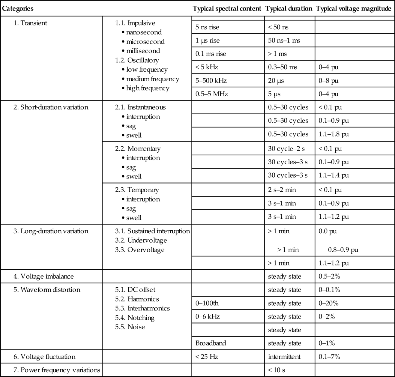
1.3.1 Transients

Power system transients are undesirable, fast- and short-duration events that produce distortions. Their characteristics and waveforms depend on the mechanism of generation and the network parameters (e.g., resistance, inductance, and capacitance) at the point of interest. “Surge” is often considered synonymous with transient.

Transients can be classified with their many characteristic components such as amplitude, duration, rise time, frequency of ringing polarity, energy delivery capability, amplitude spectral density, and frequency of occurrence. Transients are usually classified into two categories: impulsive and oscillatory (Table 1.2).

An impulsive transient is a sudden frequency change in the steady-state condition of voltage, current, or both that is unidirectional in polarity (Fig. 1.3). The most common cause of impulsive transients is a lightning current surge. Impulsive transients can excite the natural frequency of the system.

An oscillatory transient is a sudden frequency change in the steady-state condition of voltage, current, or both that includes both positive and negative polarity values. Oscillatory transients occur for different reasons in power systems such as appliance switching, capacitor bank switching (Fig. 1.4), fast-acting overcurrent protective devices, and ferroresonance (Fig. 1.5).

1.3.2 Short-Duration Voltage Variations

This category encompasses the IEC category of “voltage dips” and “short interruptions.” According to the IEEE-1159 classification, there are three different types of short-duration events (Table 1.2): instantaneous, momentary, and temporary. Each category is divided into interruption, sag, and swell. Principal cases of short-duration voltage variations are fault conditions, large load energization, and loose connections.

Interruption

Interruption occurs when the supply voltage (or load current) decreases to less than 0.1 pu for less than 1 minute, as shown by Fig. 1.6. Some causes of interruption are equipment failures, control malfunction, and blown fuse or breaker opening.

The difference between long (or sustained) interruption and interruption is that in the former the supply is restored manually, but during the latter the supply is restored automatically. Interruption is usually measured by its duration. For example, according to the European standard EN-50160 [24]:

• A short interruption is up to 3 minutes; and

• A long interruption is longer than 3 minutes.

However, based on the standard IEEE-1250 [25]:

• An instantaneous interruption is between 0.5 and 30 cycles;

• A momentary interruption is between 30 cycles and 2 seconds;

• A temporary interruption is between 2 seconds and 2 minutes; and

• A sustained interruption is longer than 2 minutes.

Sags (Dips)

Sags are short-duration reductions in the rms voltage between 0.1 and 0.9 pu, as shown by Fig. 1.7. There is no clear definition for the duration of sag, but it is usually between 0.5 cycles and 1 minute. Voltage sags are usually caused by:

• energization of heavy loads (e.g., arc furnace),

• starting of large induction motors,

• single line-to-ground faults, and

• load transferring from one power source to another.

Each of these cases may cause a sag with a special (magnitude and duration) characteristic. For example, if a device is sensitive to voltage sag of 25%, it will be affected by induction motor starting [11]. Sags are main reasons for malfunctions of electrical low-voltage devices. Uninterruptible power supply (UPS) or power conditioners are mostly used to prevent voltage sags.

Swells

The increase of voltage magnitude between 1.1 and 1.8 pu is called swell, as shown by Fig. 1.8. The most accepted duration of a swell is from 0.5 cycles to 1 minute [7]. Swells are not as common as sags and their main causes are:

• switching off of a large load,

• energizing a capacitor bank, or

• voltage increase of the unfaulted phases during a single line-to-ground fault [10].

In some textbooks the term “momentary overvoltage” is used as a synonym for the term swell. As in the case of sags, UPS or power conditioners are typical solutions to limit the effect of swell [10].

1.3.3 Long-Duration Voltage Variations

According to standards (e.g., IEEE-1159, ANSI-C84.1), the deviation of the rms value of voltage from the nominal value for longer than 1 minute is called long-duration voltage variation. The main causes of long-duration voltage variations are load variations and system switching operations. IEEE-1159 divides these events into three categories (Table 1.2): sustained interruption, undervoltage, and overvoltage.

1.3.4 Voltage Imbalance

When voltages of a three-phase system are not identical in magnitude and/or the phase differences between them are not exactly 120 degrees, voltage imbalance occurs [10]. There are two ways to calculate the degree of imbalance:

• divide the maximum deviation from the average of three-phase voltages by the average of three-phase voltages, or

• compute the ratio of the negative- (or zero-) sequence component to the positive-sequence component [7].

The main causes of voltage imbalance in power systems are:

• unbalanced single-phase loading in a three-phase system,

• overhead transmission lines that are not transposed,

• blown fuses in one phase of a three-phase capacitor bank, and

• severe voltage imbalance (e.g., > 5%), which can result from single phasing conditions.

1.3.5 Waveform Distortion

A steady-state deviation from a sine wave of power frequency is called waveform distortion [7]. There are five primary types of waveform distortions: DC offset, harmonics, interharmonics, notching, and electric noise. A Fourier series is usually used to analyze the nonsinusoidal waveform.

DC Offset

The presence of a DC current and/or voltage component in an AC system is called DC offset [7]. Main causes of DC offset in power systems are:

• employment of rectifiers and other electronic switching devices, and

• geomagnetic disturbances [6,7,13] causing GICs.

The main detrimental effects of DC offset in alternating networks are

• half-cycle saturation of transformer core [26–28],

• generation of even harmonics [26] in addition to odd harmonics [29,30],

• additional heating in appliances leading to a decrease of the lifetime of transformers [31–36], rotating machines, and electromagnetic devices, and

• electrolytic erosion of grounding electrodes and other connectors.

Figure 1.9a shows strong half-cycle saturation in a transformer due to DC magnetization and the influence of the tank, and Fig. 1.9b exhibits less half-cycle saturation due to DC magnetization and the absence of any tank. One concludes that to suppress DC currents due to rectifiers and geomagnetically induced currents, three-limb transformers with a relatively large air gap between core and tank should be used.

Harmonics

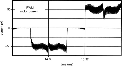
Harmonics are sinusoidal voltages or currents with frequencies that are integer multiples of the power system (fundamental) frequency (usually, f = 50 or 60 Hz). For example, the frequency of the hth harmonic is (hf). Periodic nonsinusoidal waveforms can be subjected to Fourier series and can be decomposed into the sum of fundamental component and harmonics. Main sources of harmonics in power systems are:

• industrial nonlinear loads (Fig. 1.10) such as power electronic equipment, for example, drives (Fig. 1.10a), rectifiers (Fig. 1.10b,c), inverters, or loads generating electric arcs, for example, arc furnaces, welding machines, and lighting, and

• residential loads with switch-mode power supplies such as television sets, computers (Fig. 1.11), and fluorescent and energy-saving lamps.

Some detrimental effects of harmonics are:

• maloperation of control devices,

• additional losses in capacitors, transformers, and rotating machines,

• additional noise from motors and other apparatus,

• telephone interference, and

• causing parallel and series resonance frequencies (due to the power factor correction capacitor and cable capacitance), resulting in voltage amplification even at a remote location from the distorting load.

Recommended solutions to reduce and control harmonics are applications of high-pulse rectification, passive, active, and hybrid filters, and custom power devices such as active-power line conditioners (APLCs) and unified power quality conditioners (UPQCs).

Interharmonics

Interharmonics are discussed in Section 1.4.1. Their frequencies are not integer multiples of the fundamental frequency.

Notching

A periodic voltage disturbance caused by line-commutated thyristor circuits is called notching. The notching appears in the line voltage waveform during normal operation of power electronic devices when the current commutates from one phase to another. During this notching period, there exists a momentary short-circuit between the two commutating phases, reducing the line voltage; the voltage reduction is limited only by the system impedance.

Notching is repetitive and can be characterized by its frequency spectrum (Figs. 1.10b,c). The frequency of this spectrum is quite high. Usually it is not possible to measure it with equipment normally used for harmonic analysis. Notches can impose extra stress on the insulation of transformers, generators, and sensitive measuring equipment.

Notching can be characterized by the following properties:

• Notch depth: average depth of the line voltage notch from the sinusoidal waveform at the fundamental frequency;

• Notch width: the duration of the commutation process;

• Notch area: the product of notch depth and width; and

• Notch position: where the notch occurs on the sinusoidal waveform.

Some standards (e.g., IEEE-519) set limits for notch depth and duration (with respect to the system impedance and load current) in terms of the notch depth, the total harmonic distortion THD_v of supply voltage, and the notch area for different supply systems.

Electric Noise

Electric noise is defined as unwanted electrical signals with broadband spectral content lower than 200 kHz [37] superimposed on the power system voltage or current in phase conductors, or found on neutral conductors or signal lines. Electric noise may result from faulty connections in transmission or distribution systems, arc furnaces, electrical furnaces, power electronic devices, control circuits, welding equipment, loads with solid-state rectifiers, improper grounding, turning off capacitor banks, adjustable-speed drives, corona, and broadband power line (BPL) communication circuits. The problem can be mitigated by using filters, line conditioners, and dedicated lines or transformers. Electric noise impacts electronic devices such as microcomputers and programmable controllers.

1.3.6 Voltage Fluctuation and Flicker

Voltage fluctuations are systemic variations of the voltage envelope or random voltage changes, the magnitude of which does not normally exceed specified voltage ranges (e.g., 0.9 to 1.1 pu as defined by ANSI C84.1-1982) [22,38]. Voltage fluctuations are divided into two categories:

• step-voltage changes, regular or irregular in time, and

• cyclic or random voltage changes produced by variations in the load impedances.

Voltage fluctuations degrade the performance of the equipment and cause instability of the internal voltages and currents of electronic equipment. However, voltage fluctuations less than 10% do not affect electronic equipment. The main causes of voltage fluctuation are pulsed-power output, resistance welders, start-up of drives, arc furnaces, drives with rapidly changing loads, and rolling mills.

Flicker

Flicker (Fig. 1.12) has been described as “continuous and rapid variations in the load current magnitude which causes voltage variations.” The term flicker is derived from the impact of the voltage fluctuation on lamps such that they are perceived to flicker by the human eye. This may be caused by an arc furnace, one of the most common causes of the voltage fluctuations in utility transmission and distribution systems.

1.3.7 Power–Frequency Variations

The deviation of the power system fundamental frequency from its specified nominal value (e.g., 50 or 60 Hz) is defined as power frequency variation [39]. If the balance between generation and demand (load) is not maintained, the frequency of the power system will deviate because of changes in the rotational speed of electromechanical generators. The amount of deviation and its duration of the frequency depend on the load characteristics and response of the generation control system to load changes. Faults of the power transmission system can also cause frequency variations outside of the accepted range for normal steady-state operation of the power system.

1.4.1 Harmonics

Nonsinusoidal current and voltage waveforms (Figs. 1.13 to 1.20) occur in today’s power systems due to equipment with nonlinear characteristics such as transformers, rotating electric machines, FACTS devices, power electronics components (e.g., rectifiers, triacs, thyristors, and diodes with capacitor smoothing, which are used extensively in PCs, audio, and video equipment), switch-mode power supplies, compact fluorescent lamps, induction furnaces, adjustable AC and DC drives, arc furnaces, welding tools, renewable energy sources, and HVDC networks. The main effects of harmonics are maloperation of control devices, telephone interferences, additional line losses (at fundamental and harmonic frequencies), and decreased lifetime and increased losses in utility equipment (e.g., transformers, rotating machines, and capacitor banks) and customer devices.

The periodic nonsinusoidal waveforms can be formulated in terms of Fourier series. Each term in the Fourier series is called the harmonic component of the distorted waveform. The frequency of harmonics are integer multiples of the fundamental frequency. Therefore, nonsinusoidal voltage and current waveforms can be defined as

$\begin{array}{c}v\left(t\right)=V_{DC}+{\displaystyle \sum _{h=1}^n{V}_{rms}^{\left(h\right)}}cos\left(h{\omega }_{o}t+{\alpha }_h\right)\\ =V_{DC}+v^{\left(1\right)}\left(t\right)+v^{\left(2\right)}\left(t\right)+v^{\left(3\right)}\left(t\right)+v^{\left(4\right)}\left(t\right)+\dots \dots ,\end{array}$

$\begin{array}{c}i\left(t\right)=I_{DC}+{\displaystyle \sum _{h=1}^n{I}_{rms}^{\left(h\right)}cos\left(h{\omega }_{o}t+{\beta }_h\right)}\\ =I_{DC}+i^{\left(1\right)}\left(t\right)+i^{\left(2\right)}\left(t\right)+i^{\left(3\right)}\left(t\right)+i^{\left(4\right)}\left(t\right)+\dots \dots \text{,}\end{array}$

where ω_o is the fundamental frequency, h is the harmonic order, and V_rms^(h), I_rms^(h), α_h, and β_h are the rms amplitude values and phase shifts of voltage and current for the hth harmonic.

Even and odd harmonics of a nonsinusoidal function correspond to even (e.g., 2, 4, 6, 8, …) and odd (e.g., 3, 5, 7, 9, …) components of its Fourier series. Harmonics of order 1 and 0 are assigned to the fundamental frequency and the DC component of the waveform, respectively. When both positive and negative half-cycles of the waveform have identical shapes, the wave shape has half-wave symmetry and the Fourier series contains only odd harmonics. This is the usual case with voltages and currents of power systems. The presence of even harmonics is often a clue that there is something wrong (e.g., imperfect gating of electronic switches [42]), either with the load equipment or with the transducer used to make the measurement. There are notable exceptions to this such as half-wave rectifiers, arc furnaces (with random arcs), and the presence of GICs in power systems [27].

Triplen Harmonics

Triplen harmonics (Fig. 1.21) are the odd multiples of the third harmonic (h = 3, 9, 15, 21, …). These harmonic orders become an important issue for grounded-wye systems with current flowing in the neutral line of a wye configuration. Two typical problems are overloading of the neutral conductor and telephone interference.

For a system of perfectly balanced three-phase nonsinusoidal loads, fundamental current components in the neutral are zero. The third harmonic neutral currents are three times the third-harmonic phase currents because they coincide in phase or time.

Transformer winding connections have a significant impact on the flow of triplen harmonic currents caused by three-phase nonlinear loads. For the grounded wye-delta transformer, the triplen harmonic currents enter the wye side and since they are in phase, they add in the neutral. The delta winding provides ampere-turn balance so that they can flow in the delta, but they remain trapped in the delta and are absent in the line currents of the delta side of the transformer. This type of transformer connection is the most commonly employed in utility distribution substations with the delta winding connected to the transmission feeder. Using grounded-wye windings on both sides of the transformer allows balanced triplen harmonics to flow unimpeded from the low-voltage system to the high-voltage system. They will be present in equal proportion on both sides of a transformer.

Subharmonics

Subharmonics have frequencies below the fundamental frequency. There are rarely subharmonics in power systems. However, due to the fast control of electronic power supplies of computers, inter- and subharmonics are generated in the input current (Fig. 1.11) [45]. Resonance between the harmonic currents or voltages with the power system (series) capacitance and inductance may cause subharmonics, called subsynchronous resonance [46]. They may be generated when a system is highly inductive (such as an arc furnace during start-up) or when the power system contains large capacitor banks for power factor correction or filtering.

Interharmonics

The frequency of interharmonics are not integer multiples of the fundamental frequency. Interharmonics appear as discrete frequencies or as a band spectrum. Main sources of interharmonic waveforms are static frequency converters, cycloconverters, induction motors, arcing devices, and computers. Interharmonics cause flicker, low-frequency torques [32], additional temperature rise in induction machines [33,34], and malfunctioning of protective (under-frequency) relays [35]. Interharmonics have been included in a number of guidelines such as the IEC 61000-4-7 [36] and the IEEE-519. However, many important related issues, such as the range of frequencies, should be addressed in revised guidelines.

Characteristic and Uncharacteristic Harmonics

The harmonics of orders 12 k + 1 (positive sequence) and 12 k – 1 (negative sequence) are called characteristic and uncharacteristic harmonics, respectively. The amplitudes of these harmonics are inversely proportional to the harmonic order. Filters are used to reduce characteristic harmonics of large power converters. When the AC system is weak [47] and the operation is not perfectly symmetrical, uncharacteristic harmonics appear. It is not economical to reduce uncharacteristic harmonics with filters; therefore, even a small injection of these harmonic currents can, via parallel resonant conditions, produce very large voltage distortion levels.

Positive-, Negative-, and Zero-Sequence Harmonics [48]

Assuming a positive-phase (abc) sequence balanced three-phase power system, the expressions for the fundamental currents are

$\begin{array}{l}{i}_a\left(t\right)=I_a^{\left(1\right)}cos\left({\omega }_{o}t\right)\\ i_b\left(t\right)=I_b^{\left(1\right)}cos\left({\omega }_{o}t-120°\right)\\ i_c\left(t\right)=I_c^{\left(1\right)}cos\left({\omega }_{o}t-240°\right)\end{array}$

  (1-2)

The negative displacement angles indicate that the fundamental phasors rotate clockwise in the space–time plane.

For the third harmonic (zero-sequence) currents,

$\begin{array}{c}{i}_a^{\left(3\right)}\left(t\right)=I_a^{\left(3\right)}cos\left(3{\omega }_{o}t\right)\\ i_b^{\left(3\right)}\left(t\right)=I_b^{\left(3\right)}cos3\left({\omega }_{o}t-120°\right)=I_b^{\left(3\right)}cos\left(3{\omega }_{o}t-360°\right)=I_b^{\left(3\right)}cos\left(3{\omega }_{o}t\right)\\ i_c^{\left(3\right)}\left(t\right)=I_c^{\left(3\right)}cos3\left({\omega }_{o}t-240°\right)=I_c^{\left(3\right)}cos\left(3{\omega }_{o}t-720°\right)=I_c^{\left(3\right)}cos\left(3{\omega }_{o}t\right)\end{array}$

  (1-3)

This equation shows that the third harmonic phasors are in phase and have zero displacement angles between them. The third harmonic currents are known as zero-sequence harmonics.

The expressions for the fifth harmonic currents are

$\begin{array}{l}{i}_a^{\left(5\right)}\left(t\right)=I_a^{\left(5\right)}cos\left(5{\omega }_{o}t\right)\hfill \\ i_b^{\left(5\right)}\left(t\right)=I_b^{\left(5\right)}cos5\left({\omega }_{o}t-120°\right)=I_b^{\left(5\right)}cos\left(5{\omega }_{o}t-600°\right)\\ =I_b^{\left(5\right)}cos\left(5{\omega }_{o}t-240°\right)=I_b^{\left(5\right)}cos\left(5{\omega }_{o}t+120°\right)\\ i_c^{\left(5\right)}\left(t\right)=I_c^{\left(5\right)}cos5\left({\omega }_{o}t-240°\right)=I_c^{\left(5\right)}cos\left(5{\omega }_{o}t-1200°\right)\\ =I_c^{\left(5\right)}cos\left(5{\omega }_{o}t-120°\right)=I_c^{\left(5\right)}cos\left(5{\omega }_{o}t+240°\right)\end{array}$

  (1-4)

Note that displacement angles are positive; therefore, the phase sequence of this harmonic is counterclockwise and opposite to that of the fundamental. The fifth harmonic currents are known as negative-sequence harmonics.

Similar relationships exist for other harmonic orders. Table 1.3 categorizes power system harmonics in terms of their respective frequencies and sources.

Table 1.3

Types and Sources of Power System Harmonics

Type	Frequency	Source
DC	0	Electronic switching devices, half-wave rectifiers, arc furnaces (with random arcs), geomagnetic induced currents (GICs)
Odd harmonics	h • f1 (h = odd)	Nonlinear loads and devices
Even harmonics	h • f1 (h = even)	Half-wave rectifiers, geomagnetic induced currents (GICs)
Triplen harmonics	3 h • f1 (h = 1, 2, 3, 4, …)	Unbalanced three-phase load, electronic switching devices
Positive-sequence harmonics	h • f1 (h = 1, 4, 7, 10, …)	Operation of power system with nonlinear loads
Negative-sequence harmonics	h • f1 (h = 2, 5, 8, 11, …)	Operation of power system with nonlinear loads
Zero-sequence harmonics	h • f1 (h = 3, 6, 9, 12, …)(same as triplen harmonics)	Unbalanced operation of power system
Time harmonics	h • f1 (h = an integer)	Voltage and current source inverters, pulse-width-modulated rectifiers, switch-mode rectifiers and inverters
Spatial harmonics	h • f1 (h = an integer)	Induction machines
Interharmonic	h • f1 (h = not an integer multiple of f1)	Static frequency converters, cycloconverters, induction machines, arcing devices, computers
Subharmonic	h • f1 (h < 1 and not an integer multiple of f1, e.g., h = 15 Hz, 30 Hz)	Fast control of power supplies, subsynchronous resonances, large capacitor banks in highly inductive systems, induction machines
Characteristic harmonic	(12 k + 1) • f1 (k = integer)	Rectifiers, inverters
Uncharacteristic harmonic	(12 k – 1) • f1 (k = integer)	Weak and unsymmetrical AC systems

Note that although the harmonic phase-shift angle has the effect of altering the shape of the composite waveform (e.g., adding a third harmonic component with 0 degree phase shift to the fundamental results in a composite waveform with maximum peak-to-peak value whereas a 180 degree phase shift will result in a composite waveform with minimum peak-to-peak value), the phase–sequence order of the harmonics is not affected. Not all voltage and current systems can be decomposed into positive-, negative-, and zero-sequence systems [49].

Time and Spatial (Space) Harmonics

Time harmonics are the harmonics in the voltage and current waveforms of electric machines and power systems due to magnetic core saturation, presence of nonlinear loads, and irregular system conditions (e.g., faults and imbalance). Spatial (space) harmonics are referred to the harmonics in the flux linkage of rotating electromagnetic devices such as induction and synchronous machines. The main cause of spatial harmonics is the unsymmetrical physical structure of stator and rotor magnetic circuits (e.g., selection of number of slots and rotor eccentricity). Spatial harmonics of flux linkages will induce time harmonic voltages in the rotor and stator circuits that generate time harmonic currents.

1.4.2 The Average Value of a Nonsinusoidal Waveform

The average value of a sinusoidal waveform is defined as

$I_{ave}=\frac{1}{T}{\displaystyle \underset{0}{\overset{T}{\int }}i\left(t\right)dt\text{.}}$

For the nonsinusoidal current of Eq. 1-1,

$\begin{array}{c}{I}_{ave}=\frac{1}{T}{\displaystyle \underset{0}{\overset{T}{\int }}i\left(t\right)dt}=\frac{1}{T}{\displaystyle \underset{0}{\overset{T}{\int }}\left[I_{DC}+i^{\left(1\right)}\left(t\right)+i^{\left(2\right)}\left(t\right)+i^{\left(3\right)}\left(t\right)+i^{\left(4\right)}\left(t\right)+.\dots .\right]dt\text{.}}\end{array}$

Since all harmonics are sinusoids, the average value of a nonsinusoidal function is equal to its DC value:

$I_{ave}=I_{DC\cdot }$

1.4.3 The rms Value of a Nonsinusoidal Waveform

The rms value of a sinusoidal waveform is defined as

$\begin{array}{c}{I}_{rms}=\sqrt{\frac{1}{T}{\displaystyle \underset{0}{\overset{T}{\int }}{i}^2\left(t\right)dt}}=\sqrt{\frac{1}{2\pi }{\displaystyle \underset{0}{\overset{T}{\int }}{I}_{\text{max}}^2{cos}^2\left(\omega t\right)dt}}=\sqrt{\frac{1}{2}{I}_{\text{max}}^2}=\frac{I_{\text{max}}}{\sqrt{2}}\text{.}\end{array}$

For the nonsinusoidal current of Eq. 1-1,

$\begin{array}{c}{I}_{rms}=\sqrt{\frac{1}{T}{\displaystyle \underset{0}{\overset{T}{\int }}{i}^2\left(t\right)dt}}\\ ={\left\{\frac{1}{T}{\displaystyle \underset{0}{\overset{T}{\int }}{\left[I_{\text{max}}^{\left(1\right)}cos\left(\omega t+{\beta }_1\right)+I_{\text{max}}^{\left(2\right)}cos\left(2\omega t+{\beta }_2\right)+I_{\text{max}}^{\left(3\right)}cos\left(3\omega t+{\beta }_3\right)+\dots \right]}^{2}dt}\right\}}^{1/2}\\ =\left\{\frac{1}{T}{\displaystyle \underset{0}{\overset{T}{\int }}\left[{\left(I_{\text{max}}^{\left(1\right)}\right)}^2{cos}^2(\omega t+{\beta }_1\right)}\right.+{\left(I_{\text{max}}^{\left(2\right)}\right)}^2{cos}^2\left(2\omega t+{\beta }_2\right)\\ +{\left(I_{\text{max}}^{\left(3\right)}\right)}^2{cos}^2\left(3\omega t+{\beta }_3\right)+\dots +2I_{\text{max}}^{\left(1\right)}\cdot \\ {\left.I_{\text{max}}^{\left(2\right)}cos\left(\omega t+{\beta }_1\right)cos\left(2\omega t+{\beta }_2\right)+\dots ]dt\right\}}^{1/2}\text{.}\end{array}$

This equation contains two parts:

• The first part is the sum of the squares of harmonics:

${\displaystyle \sum _{p=1}^H{\left(I_{\text{max}}^{\left(p\right)}\right)}^2{cos}^2\left(p\omega t+{\beta }_p\right)\text{.}}$

• The second part is the sum of the products of harmonics:

${\displaystyle \sum _{p=1}^H{\displaystyle \sum _{q=1}^H{I}_{\text{max}}^{\left(p\right)}{I}_{\text{max}}^{\left(q\right)}cos\left(p\omega t+{\beta }_p\right)cos\left(q\omega t+{\beta }_q\right),p\ne q\text{.}}}$

After some simplifications it can be shown that the average of the second part is zero, and the first part becomes

$\begin{array}{c}{I}_{rms}={\displaystyle \underset{0}{\overset{2\pi }{\int }}\left[{\displaystyle \sum _{p=1}^H{\left(I_{\text{max}}^{\left(p\right)}\right)}^2{cos}^2\left(p\omega t+{\beta }_p\right)}\right]}d\left(p\omega t\right)\\ ={\displaystyle \underset{0}{\overset{2\pi }{\int }}\left[{\left(I_{\text{max}}^{\left(1\right)}\right)}^{2}cos\left(\omega t+{\beta }_1\right)\right]d\left(\omega t\right)}+\left[{\displaystyle \underset{0}{\overset{2\pi }{\int }}{\left(I_{\text{max}}^{\left(2\right)}\right)}^{2}cos\left(2\omega t+{\beta }_2\right)}\right]d\left(2\omega t\right)+\dots .\end{array}$

Therefore, the rms value of a nonsinusoidal waveform is

$I_{rms}={\left[{\left(I_{rms}^{\left(1\right)}\right)}^2+{\left(I_{rms}^{\left(2\right)}\right)}^2+{\left(I_{rms}^{\left(3\right)}\right)}^2+\dots +{\left(I_{rms}^{\left(H\right)}\right)}^2\right]}^{1/2}\text{.}$

If the nonsinusoidal waveform contains DC values, then

$I_{rms}={\left[I_{DC}+{\left(I_{rms}^{\left(1\right)}\right)}^2+{\left(I_{rms}^{\left(2\right)}\right)}^2+{\left(I_{rms}^{\left(3\right)}\right)}^2+\dots +{\left(I_{rms}^{\left(H\right)}\right)}^2\right]}^{1/2}\text{.}$

1.4.4 Form Factor (FF)

The form factor (FF) is a measure of the shape of the waveform and is defined as

$FF=\frac{I_{rms}}{I_{ave}}\text{.}$

Since the average value of a sinusoid is zero, its average over one half-cycle is used in the above equation. As the harmonic content of the waveform increases, its FF will also increase.

1.4.5 Ripple Factor (RF)

Ripple factor (RF) is a measure of the ripple content of the waveform and is defined as

$RF=\frac{I_{\mathit{AC}}}{I_{DC}}\text{,}$

where $I_{\mathit{AC}}=\sqrt{{\left(I_{rms}\right)}^2-{\left(I_{DC}\right)}^2}\text{.}$ It is easy to show that

$\begin{array}{l}RF=\frac{\sqrt{{\left(I_{rms}\right)}^2-{\left(I_{DC}\right)}^2}}{I_{DC}}=\sqrt{\frac{{\left(I_{rms}\right)}^2}{{\left(I_{DC}\right)}^2}-\frac{{\left(I_{DC}\right)}^2}{{\left(I_{DC}\right)}^2}}=\sqrt{F{F}^2-1}\text{.}\end{array}$

1.4.6 Harmonic Factor (HF_h)

The harmonic factor (HF_h) of the hth harmonic, which is a measure of the individual harmonic contribution, is defined as

$H{F}_h=\frac{I_{rms}^{\left(h\right)}}{I_{rms}^{\left(1\right)}}\text{.}$

Some references [8] call HF_h the individual harmonic distortion (IHD).

1.4.7 Lowest Order Harmonic (LOH)

The lowest order harmonic (LOH) is that harmonic component whose frequency is closest to that of the fundamental and its amplitude is greater than or equal to 3% of the fundamental component.

1.4.8 Total Harmonic Distortion (THD)

The most common harmonic index used to indicate the harmonic content of a distorted waveform with a single number is the total harmonic distortion (THD). It is a measure of the effective value of the harmonic components of a distorted waveform, which is defined as the rms of the harmonics expressed in percentage of the fundamental (e.g., current) component:

$TH{D}_i=\frac{\sqrt{{\displaystyle \sum _{h=2}^{\infty }{\left(I^{\left(h\right)}\right)}^2}}}{I^{\left(1\right)}}\text{.}$

A commonly cited value of 5% is often used as a dividing line between a high and low distortion level. The ANSI standard recommends truncation of THD series at 5 kHz, but most practical commercially available instruments are limited to about 1.6 kHz (due to the limited bandwidth of potential and current transformers and the word length of the digital hardware [5]).

Main advantages of THD are:

• It is commonly used for a quick measure of distortion; and

• It can be easily calculated.

Some disadvantages of THD are:

• It does not provide amplitude information; and

• The detailed information of the spectrum is lost.

THD_i is related to the rms value of the current waveform as follows [6]:

$I_{rms}=\sqrt{{\displaystyle \sum _{h=2}^{\infty }{\left(I^{\left(h\right)}\right)}^2}}=I^{\left(1\right)}\sqrt{1+TH{D}_i^2}\text{.}$

THD can be weighted to indicate the amplitude stress on various system devices. The weighted distortion factor adapted to inductance is an approximate measure for the additional thermal stress of inductances of coils and induction motors [9, Table 2.4]:

THD adapted to inductance = THD_ind

$=\frac{\sqrt{{\displaystyle \sum _{h=2}^{50}\left(\frac{{\left(V^{\left(h\right)}\right)}^2}{h^{\alpha }}\right)}}}{V^{\left(1\right)}}\text{,}$

where α = 1 … 2. On the other hand, the weighted THD adapted to capacitors is an approximate measure for the additional thermal stress of capacitors directly connected to the system without series inductance [9, Table 2.4]:

THD adapted to capacitor = THD_cap

$=\frac{\sqrt{{\displaystyle \sum _{h=2}^{50}\left(h\times {\left(V^{\left(h\right)}\right)}^2\right)}}}{V^{\left(1\right)}}\text{.}$

Because voltage distortions are maintained small, the voltage THD_v nearly always assumes values which are not a threat to the power system. This is not the case for current; a small current may have a high THD_i but may not be a significant threat to the system.

1.4.9 Total Interharmonic Distortion (TIHD)

This factor is equivalent to the (e.g., current) THD_i, but is defined for interharmonics as [9]

$\mathit{TIHD}=\frac{\sqrt{{\displaystyle \sum _{k=1}^n{\left(I^{\left(k\right)}\right)}^2}}}{I^{\left(1\right)}}\text{,}$

where k is the total number of interharmonics and n is the total number of frequency bins present including subharmonics (e.g., interharmonic frequencies that are less than the fundamental frequency).

1.4.10 Total Subharmonic Distortion (TSHD)

This factor is equivalent to the (e.g., current) THD_i, but defined for subharmonics [9]:

$\mathit{TSHD}=\frac{\sqrt{{\displaystyle \sum _{s=1}^s{\left(I^{\left(s\right)}\right)}^2}}}{I^{\left(1\right)}}\text{,}$

where s is the total number of frequency bins present below the fundamental frequency.

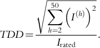
1.4.11 Total Demand Distortion (TDD)

Due to the mentioned disadvantages of THD, some standards (e.g., IEEE-519) have defined the total demand distortion factor. This term is similar to THD except that the distortion is expressed as a percentage of some rated or maximum value (e.g., load current magnitude), rather than as a percentage of the fundamental current:

$TDD=\frac{\sqrt{{\displaystyle \sum _{h=2}^{50}{\left(I^{\left(h\right)}\right)}^2}}}{I_{\mathrm{rated}}}\text{.}$

1.4.12 Telephone Influence Factor (TIF)

The telephone influence factor (TIF), which was jointly proposed by Bell Telephone Systems (BTS) and the Edison Electric Institute (EEI) and is widely used in the United States and Canada, determines the influence of power systems harmonics on telecommunication systems. It is a variation of THD in which the root of the sum of the squares is weighted using factors (weights) that reflect the response of the human ear [5]:

$TIF=\frac{\sqrt{{\displaystyle \sum _{i=1}^{\infty }{\left(w_i{V}^{\left(i\right)}\right)}^2}}}{\sqrt{{\displaystyle \sum _{i=1}^{\infty }{\left(V^{\left(i\right)}\right)}^2}}}\text{,}$

where w_i are the TIF weighting factors obtained by physiological and audio tests, as listed in Table 1.4. They also incorporate the way current in a power circuit induces voltage in an adjacent communication system.

1.4.13 C-Message Weights

The C-message weighted index is very similar to the TIF except that the weights c_i are used in place of w_i [5]:

$C=\frac{\sqrt{{\displaystyle \sum _{i=1}^{\infty }{\left(c_i{I}^{\left(i\right)}\right)}^2}}}{\sqrt{{\displaystyle \sum _{i=1}^{\infty }{\left(I^{\left(i\right)}\right)}^2}}}=\frac{\sqrt{{\displaystyle \sum _{i=1}^{\infty }{\left(c_i{I}^{\left(i\right)}\right)}^2}}}{I_{rms}}\text{,}$

where c_i are the C-message weighting factors (Table 1.4) that are related to the TIF weights by w_i = 5(i)(f₀)c_i. The C-message could also be applied to the bus voltage.

1.4.14 V · T and I · T Products

The THD index does not provide information about the amplitude of voltage (or current); therefore, BTS or the EEI use I · T and V · T products. The I · T and V · T products are alternative indices to the THD incorporating voltage or current amplitudes:

$V\cdot T=\sqrt{{\displaystyle \sum _{i=1}^{\infty }{\left(w_i{V}^{\left(1\right)}\right)}^2}}\text{,}$

$I\cdot T=\sqrt{{\displaystyle \sum _{i=1}^{\infty }{\left(w_i{I}^{\left(i\right)}\right)}^2}}\text{,}$

where the weights w_i are listed in Table 1.4.

1.4.15 Telephone Form Factor (TFF)

Two weighting systems widely used by industry for interference on telecommunication system are [9]:

• the sophomoric weighting system proposed by the International Consultation Commission on Telephone and Telegraph System (CCITT) used in Europe, and

• the C-message weighting system proposed jointly by Bell Telephone Systems (BTS) and the Edison Electric Institute (EEI), used in the United States and Canada.

These concepts acknowledge that the harmonic effect is not uniform over the audio-frequency range and use measured weighting factors to account for this nonuniformity. They take into account the type of telephone equipment and the sensitivity of the human ear to provide a reasonable indication of the interference from each harmonic.

The BTS and EEI systems describe the level of harmonic interference in terms of the telephone influence factor (Eq. 1-26) or the C-message (Eq. 1-27), whereas the CCITT system uses the telephone form factor (TFF):

$TFF=\frac{1}{V^{\left(1\right)}}\sqrt{{\displaystyle \sum _{h=1}^{\infty }{K}_h{P}_h{\left(V^{\left(h\right)}\right)}^2}}\text{,}$

where K_h = h/800 is a coupling factor and P_h is the harmonic weight [9 (Fig. 2.5)] divided by 1000.

1.4.16 Distortion Index (DIN)

The distortion index (DIN) is commonly used in standards and specifications outside North America. It is also used in Canada and is defined as [5]

$DIN=\frac{\sqrt{{\displaystyle \sum _{i=2}^{\infty }{\left(V^{\left(i\right)}\right)}^2}}}{\sqrt{{\displaystyle \sum _{i=1}^{\infty }{\left(V^{\left(i\right)}\right)}^2}}}=\frac{THD}{\sqrt{TH{D}^2+1}}\text{.}$

For low levels of harmonics, a Taylor series expansion can be applied to show

$DIN\approx THD\left(1-\frac{1}{2}THD\right)\text{.}$

1.4.17 Distortion Power (D)

Harmonic distortion complicates the computation of power and power factors because voltage and current equations (and their products) contain harmonic components. Under sinusoidal conditions, there are four standard quantities associated with power:

• Fundamental apparent power (S₁) is the product of the rms fundamental voltage and current;

• Fundamental active power (P₁) is the average rate of delivery of energy;

• Fundamental reactive power (Q₁) is the portion of the apparent power that is oscillatory; and

• Power factor at fundamental frequency (or displacement factor) cos θ₁ = P₁/S₁.

The relationship between these quantities is defined by the power triangle:

${\left(S_1\right)}^2={\left(P_1\right)}^2+{\left(Q_1\right)}^2\text{.}$

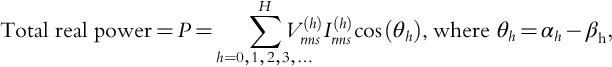
If voltage and current waveforms are nonsinusoidal (Eq. 1-1), the above equation does not hold because S contains cross terms in the products of the Fourier series that correspond to voltages and currents of different frequencies, whereas P and Q correspond to voltages and currents of the same frequency. It has been suggested to account for these cross terms as follows [5,50,51]:

$S^2=P^2+Q^2+D^2\text{,}$

where

Apparent power = S = V_rmsI_rms

$=\sqrt{{\displaystyle \sum _{h=0,1,2,3,\dots }^H{\left(V_{rms}^{\left(h\right)}\right)}^2}}\sqrt{{\displaystyle \sum _{h=0,1,2,3,\dots }^H{\left(I_{rms}^{\left(h\right)}\right)}^2}}\text{,}$

$\mathrm{Total}\mathrm{real}\mathrm{power}=P={\displaystyle \sum _{h=0,1,2,3,\dots }^H{V}_{rms}^{\left(h\right)}}{I}_{rms}^{\left(h\right)}cos\left({\theta }_h\right),\mathrm{where}{\theta }_h={\alpha }_h–{\beta }_{\mathrm{h}}\text{,}$

$\mathrm{Total}\mathrm{reactive}\mathrm{power}=Q={\displaystyle \sum _{h=0,1,2,3,\dots }^H{V}_{rms}^{\left(h\right)}}{I}_{rms}^{\left(h\right)}sin\left({\theta }_h\right)\text{,}$

$\mathrm{Distortion}\mathrm{power}=D={\displaystyle \sum _{m=0}^{H-1}{\displaystyle \sum _{n=m+1}^H[{\left(V_{rms}^{\left(m\right)}\right)}^2{\left(I_{rms}^{\left(n\right)}\right)}^2}}+\left(V_{rms}^{\left(n\right)}\right){}^2{\left(I_{rms}^{\left(m\right)}\right)}^2-2V_{rms}^{\left(m\right)}{I}_{rms}^{\left(n\right)}cos\left({\theta }_m-{\theta }_n\right)]\text{.}$

Also, the fundamental power factor (displacement factor) in the case of sinusoidal voltage and nonsinusoidal currents is defined as [8]

$cos{\theta }_1=\frac{P_1}{\sqrt{{\left(P_1\right)}^2+{\left(Q_1\right)}^2}}\text{,}$

and the harmonic displacement factor is defined as [8]

$\lambda =\frac{P_1}{\sqrt{{\left(P_1\right)}^2+{\left(Q_1\right)}^2+D^2}}\text{.}$

The power and displacement factor quantities are shown in addition to the power quantities in Fig. 1.22. A detailed comparison of various definitions of the distortion power D is given in reference [51].

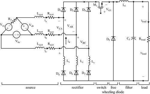
1.4.18 Application Example 1.1: Calculation of Input/Output Currents and Voltages of a Three-Phase Thyristor Rectifier

The circuit of Fig. E1.1.1 represents a phase-controlled, three-phase thyristor rectifier. The balanced input line-to-line voltages are v_ab = $\sqrt{2}240$ sin ωt, v_bc = $\sqrt{2}240$ sin(ωt – 120°), and v_ca = $\sqrt{2}240$ sin(ωt – 240°), where ω = 2πf and f = 60 Hz. Each of the six thyristors can be modeled by a self-commutated electronic switch and a diode in series, as is illustrated in Fig. E1.1.2. Use the following PSpice models for the MOSFET and the diode:

• Model for self-commutated electronic switch (MOSFET):

.model SMM NMOS(Level = 3 Gamma = 0

+ Delta = 0 Eta = 0 Theta = 0 Kappa = 0 Vmax = 0

+ XJ = 0 TOX = 100 N UO = 600 PHI = 0.6 RS = 42.69 m KP = 20.87 u L = 2 u

+ W = 2.9 VTO = 3.487 RD = 0.19 CBD = 200 n PB = 0.8 MJ = 0.5 CGSO = 3.5 n

+ CGDO = 100 p RG = 1.2 IS = 10 f)

• Model for diode:

.model D1N4001 D(IS = 10^–12)

The parameters of the circuit are as follows:

• System resistance and inductance L_syst = 300 μH, R_syst = 0.05 Ω;

• Load resistance R_load = 10 Ω;

• Filter capacitance and inductance C_f = 500 μF, L_f = 5 mH;

• Snubber inductance L_s = 5 nH;

Note that R₃ must be nonzero because PSpice cannot accept three voltage sources connected within a loop.

Perform a PSpice analysis plotting input line-to-line voltages v_ab, v_bc, v_ca, V_ab, v_BC, v_ca, input currents i_a, i_b, i_c, and the rectified output voltage v_load and output current i_load for α = 0° during the time interval 0 ≤ t ≤ 60 ms. Print the input program. Repeat the computation for α = 50° and α = 150°.

Solution to Application Example 1.1

The PSpice program codes are provided in Table E1.1.1. Plots of input current i_a (top), line-to-line voltage v_AB (second from top), line-to-line voltages v_ab, v_bc, v_ca, and output voltage v_load for a firing angle of α = 50° are shown in Fig. E1.1.3.

1.4.19 Application Example 1.2: Calculation of Input/Output Currents and Voltages of a Three-Phase Rectifier with One Self-Commutated Electronic Switch

An inexpensive and popular rectifier is illustrated in Fig. E1.2.1. It consists of four diodes and one self-commutated electronic switch operated at, for example, f_switch = 600 Hz. The balanced input line-to-line voltages are v_ab = $\sqrt{2}240$ sin ωt, v_bc = $\sqrt{2}240$ sin(ωt – 120°), and v_ca = $\sqrt{2}240$ sin(ωt – 240°), where ω = 2πf and f = 60 Hz. Perform a PSpice analysis. Use the following PSpice models for the MOSFET and the diodes:

• Model for self-commutated electronic switch (MOSFET):

. MODEL SMM NMOS(LEVEL = 3 GAMMA = 0 DELTA = 0 ETA = 0 THETA = 0

+ KAPPA = 0 VMAX = 0 XJ = 0 TOX = 100 n UO = 600 PHI = 0.6 RS = 42.69 M + KP = 20.87 u

+ L = 2 u W = 2.9 VTO = 3.487 RD = 0.19 CBD = 200 n PB = 40.8 MJ = 0.5 + CGSO = 3.5 n

+ CGDO = 100 p RG = 1.2 IS = 10 f)

• Model for diode:

.MODEL D1N4001 D(IS = 10^–12)

The parameters of the circuit are as follows:

• System resistance and inductance L_syst = 10 mH, R_syst = 0.05 Ω;

• Load resistance R_load = 10 Ω;

• Filter capacitance and inductance C_f = 500 μF, L_f = 5 mH; and

• Snubber inductance L_s = 5 nH.

Note that R₃ must be nonzero because PSpice cannot accept three voltage sources connected within a loop. The freewheeling diode is required to reduce the voltage stress on the self-commutated switch.

Print the PSpice input program. Perform a PSpice analysis plotting input line-to-line voltages v_ab, v_bc, v_ca, v_AB, v_bc, v_ca ,input currents i_a, i_b, i_c, and the rectified output voltage v_load and output current i_load for a duty ratio of δ = 50% during the time interval 0 ≤ t ≤ 60 ms.

Solution to Application Example 1.2

The PSpice program codes are provided in Table E1.2.1. Plots of input line current i_a (top), line-to-line voltage v_AB with (extreme) commutating notches (second from top), line-to-line voltages v_ab, v_bc, and v_ca are shown in Fig. E1.2.2.

1.4.20 Application Example 1.3: Calculation of Input Currents of a Brushless DC Motor in Full-on Mode (Three-Phase Permanent-Magnet Motor Fed by a Six-Step Inverter)

In the drive circuit of Fig. E1.3.1 the DC input voltage is V_DC = 300 V. The inverter is a six-pulse or six-step or full-on inverter consisting of six self-commutated (e.g., MOSFET) switches. The electric machine is a three-phase permanent-magnet motor represented by induced voltages (e_A, e_B, e_C), resistances, and leakage inductances (with respect to stator phase windings) for all three phases. The induced voltage of the stator winding (phase A) of the permanent-magnet motor is

$e_A=160sin\left(\omega t+\theta \right)$

where ω = 2πf₁ and f₁ = 1500 Hz. Correspondingly,

$e_B=160sin\left(\omega t+240°+\theta \right)$

$e_C=160sin\left(\omega t+120°+\theta \right)$

The resistance R₁ and the leakage inductance L_1ℓ of one of the phases are 0.5 Ω and 50 μH, respectively.

The magnitude of the gating voltages of the six MOSFETs is V_Gmax = 15 V. The gating signals with their phase sequence are shown in Fig. E1.3.2. Note that the phase sequence of the induced voltages (e_A, e_B, e_C) and that of the gating signals (see Fig. E1.3.2) must be the same. If these phase sequences are not the same, then no periodic solution for the machine currents (i_MA, i_MB, i_MC) can be obtained.

The models of the enhancement metal-oxide semiconductor field-effect transistors and those of the (external) freewheeling diodes are as follows:

• Model for self-commutated electronic switch (MOSFET):

.MODEL SMM NMOS(LEVEL = 3 GAMMA = 0

+ DELTA = 0 ETA = 0 THETA = 0

+ KAPPA = 0 VMAX = 0 XJ = 0 TOX = 100 n UO = 600 PHI = 0.6 RS = 42.69 M + KP = 20.87 u

+ L = 2 u W = 2.9 VTO = 3.487 RD = 0.19 CBD = 200 n PB = 0.8 MJ = 0.5 + CGSO = 3.5 n

+ CGDO = 100 p RG = 1.2 IS = 10 f)

• Model for diode:

.MODEL D1N4001 D(IS = 10^–12)

a) Using PSpice, compute and plot the current of MOSFET Q_Au (e.g., i_qau) and the motor current of phase A (e.g., i_MA) for the phase angles of the induced voltages θ = 0°, θ = + 30°, θ = + 60°, θ = –30°, and θ = –60°. Note that the gating signal frequency of the MOSFETs corresponds to the frequency f₁, that is, full-on mode operation exists. For switching sequence see Fig. E1.3.2.

b) Repeat part a for θ = + 30° with reversed-phase sequence.

Note the following:

• The step size for the numerical solution should be in the neighborhood of Δt = 0.05 μs; and

• To eliminate computational transients due to inconsistent initial conditions compute at least three periods of all quantities and plot the last (third) period of i_qau and i_MA for all five cases, where θ assumes the values given above.

Solution to Application Example 1.3

a) The PSpice program codes are provided in Table E1.3.1. Plots of MOSFET and motor currents for phase angles of θ = 0°, 30°, 60° and -60°are shown in Figs. E1.3.3a to E1.3.3d.

b) The reversed-phase: (e.g., where e_subscript_A and e_subscript_B are interchanged) sequence will result in nonperiodic waveshapes, and thus this solution is not meaningful.

1.4.21 Application Example 1.4: Calculation of the Efficiency of a Polymer Electrolyte Membrane (PEM) Fuel Cell Used as Energy Source for a Variable-Speed Drive

a) Calculate the power efficiency of a PEM fuel cell.

b) Find the specific power density of this PEM fuel cell expressed in W/kg-force.

c) How does this specific power density compare with that of a lead–acid battery [66]?

Hints:

• The nominal energy density of hydrogen is 28 kWh/kg-force, which is significantly larger than that of gasoline (12.3 kWh/kg-force). This makes hydrogen a desirable fuel for automobiles.

• The weight density of hydrogen is γ = 0.0899 g-force/liter.

• The oxygen atom has 8 electrons, 8 protons, and 8 neutrons.

A PEM fuel cell as specified by [65] has the following parameters:

Solution to Application Example 1.4

a) The power efficiency is defined by

${\eta }_{\mathrm{power}}=\left(\mathrm{rated}\mathrm{electrical}\mathrm{output}\mathrm{power}\right)/\left(\mathrm{hydrogen}\mathrm{input}\mathrm{power}\right)=P_{\mathrm{out}}/P_{\mathrm{in}}\text{.}$

Method #1. The PEM fuel cell generates 0.87 liters or 0.87 kg-force of water per hour by converting hydrogen and oxygen according to the relation

$2{\mathrm{H}}_2+{\mathrm{O}}_2=2{\mathrm{H}}_2\mathrm{O}\text{.}$

The atomic weights are

$\begin{array}{l}1\mathrm{H}\stackrel{\wedge}{=}1.0080,\\ 1\mathrm{O}\stackrel{\wedge}{=}16.0000,\\ 1{\mathrm{H}}_2\mathrm{O}\stackrel{\wedge}{=}18.0160\text{,}\end{array}$

The required weight of hydrogen to generate 0.87 liters of water per hour is $\frac{2}{18.0160}$ × 0.87 kg-force = 0.09658 kg-force. The energy input per hour in form of hydrogen is (0.09658 kg-force)(28 kWh/kg-force) = 2704.26 Wh.
Output (electrical) power of PEM fuel cell P_out = 1200 W.

Input (hydrogen) power (or energy per hour) of PEM fuel cell P_in = 2704.26 W.

Power (energy per hour) efficiency η_power = P_out/P_in = 0.4437 pu ≈ 44.4%.

Method #2. Hydrogen input power of PEM fuel cell is

${\mathrm{P}}_{\mathrm{in}}=\left(\mathrm{weight}\mathrm{density}\mathrm{of}\mathrm{hydrogen}\right)\times \left(\mathrm{hydrogen}\mathrm{consumption}\mathrm{during}\mathrm{one}\mathrm{hour}\right)\times \left(\mathrm{energy}\mathrm{density}\mathrm{of}\mathrm{hydrogen}\right)\text{.}$

With (hydrogen consumption during one hour) = 18.5 SLPM × 60 minutes/hour = (18.5)(60) liters/hour = 1110 liters/hour, one obtains the input power in form of hydrogen:

P_in = (0.0899·10^–3 kg-force /liter) (1110 liters/hour) (28·10³ W/kg-force) = 2794 W.

Power (energy per hour) efficiency

η_power = P_out/P_in = 0.4295 pu ≈ 43%.

Conclusion. Both methods generate about the same efficiency for a PEM fuel cell.

b) The specific power density of this PEM fuel cell expressed in W/kg-force is defined as

$\frac{P_{\mathrm{out}}}{\mathrm{weight}}=1200\mathrm{W}/13\mathrm{kg}-\mathrm{force}=92.3\mathrm{W}/\mathrm{kg}-\mathrm{force}\text{.}$

c) The specific power density of a PEM fuel cell is 92.3 W/kg-force as compared with that of a lead-acid battery of about 150 W/kg-force [66].

1.4.22 Application Example 1.5: Calculation of the Currents of a Wind-Power Plant PWM Inverter Feeding Power into the Power System

The circuit diagram of PWM inverter feeding power into the 240 V_L-L three-phase utility system is shown in Fig. E1.5.1 consisting of DC source, inverter, filter, and power system. The associated control circuit is given by a block diagram in Fig. E1.5.2.

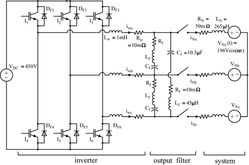
Use the PSpice program (windpower.cir) listed in Table E1.5.1.

a) Use “reverse” engineering and identify the nodes of Figs. E1.5.1 and E1.5.2, as used in the PSpice program. It may be advisable that you draw your own detailed circuit.

b) Study the PSpice program wr.cir. In particular it is important that you understand the poly statements and the subcircuit for the comparator. You may ignore the statements for the filter between switch and inverter (see Fig. E1.5.1) if the node number exceeds the maximum number of 64 (note the student version of the PSpice program is limited to a maximum of 64 nodes).

c) Run this program with inverter inductance values of L_w = 1 mH for a DC voltage of V_DC = 450 V.

d) Plot the current supplied by the inverter to the power system I(L_W1), the reference current vref1 = V(12)-V(0), and the phase power system’s voltage Vout1 = V(19)-V(123).

Solution to Application Example 1.5

The solution is presented in Fig. E1.5.3.

1.6.1 IEC 61000 Series of Standards for Power Quality

The IEC 61000 (or EN 61000) series [54], one of the most commonly used references for power quality in Europe, contains six parts, each with standards and technical reports [9]:

• Part 1 (General). Two sections cover application and interpretation aspects of EMC (electromagnetic compatibility).

• Part 2 (Environment). Twelve sections give classification of the electromagnetic environment and compatibility levels for different environments. Some aspects of this document include harmonic compatibility levels of residential LV (low voltage) systems (IEC 61000-2-2), industrial plants (IEC 61000-24), and residential MV (medium voltage) systems (IEC 61000-2-12).

• Part 3 (Limits). Eleven sections cover emission limits for harmonics and other disturbances. Some aspects of this document include harmonic current emission limits for equipment connected at LV with low (less than 16 A per phase) current (IEC 61000-3-2), flicker (IEC 61000-3-3), harmonic current emission limits for equipment connected at LV with high (more than 16 A per phase) current (IEC 61000-3-4), and assessment of emission limits for distorting loads in MV and HV (high voltage) power systems (IEC 61000-3-6).

• Part 4 (Testing and Measurement Techniques). Thirty-one sections describe standard methods for testing equipment of emission and immunity to different disturbances. Some aspects of this document include harmonic and interharmonic measurements and instrumentation (IEC 61000-4-7), dips and interruptions (EN 61000-4-11), interharmonics (EN 61000-4-13), and power quality measurement methods (IEC 61000-4-30).

• Part 5 (Installation and Mitigation Guidelines). Seven sections cover earthing (grounding), cabling, mitigation, and degrees of protection against EM (electromagnetic) disturbances.

• Part 6 (Generic Standards). Five sections cover immunity and emission standards for residential, commercial, industrial, and power station environments.

EN 61000-3-2 [2] introduces power quality limits (Table 1.6) for four classes of equipment:

• Class A: Balanced three-phase equipment and all other equipment, except those listed in other classes.

• Class B: Portable tools.

• Class C: Lighting equipment, including dimming devices.

• Class D: Equipment with a “special wave shape” and an input power of 75 to 600 W.

1.6.2 IEEE-519 Standard

The United States (ANSI and IEEE) do not have such a comprehensive and complete set of power quality standards as the IEC. However, their standards are more practical and provide theoretical background on the phenomena. This has made them very useful reference documents, even outside of the United States. IEEE-Std 519 [1] is the IEEE recommended practices and requirements for harmonic control in electric power systems. It is one of the well-known documents for power quality limits. IEEE-519 is more comprehensive than IEC 61000-3-2 [2], but it is not a product standard. The first official version of this document was published in 1981. Product testing standards for the United States are now considered within TC77A/WG1 (TF5b) but are also discussed in IEEE. The current direction of the TC-77 working group is toward a global IEC standard for both 50/60 Hz and 115/230 V.

IEEE-519 contains thirteen sections, each with standards and technical reports [11]:

• Section 1 (Introduction and Scope). Includes application of the standards.

• Section 2 (Definition and Letter Symbols).

• Section 3 (References). Includes standard references.

• Section 4 (Converter Theory and Harmonic Generation). Includes documents for converters, arc furnaces, static VAr compensators, inverters for dispersed generation, electronic control, transformers, and generators.

• Section 5 (System Response Characteristics). Includes resonance conditions, effect of system loading, and typical characteristics of industrial, distribution, and transmission systems.

• Section 6 (Effect of Harmonics). Detrimental effects of harmonics on motors, generators, transformers, capacitors, electronic equipments, meters, relaying, communication systems, and converters.

• Section 7 (Reactive Power Compensation and Harmonic Control). Discusses converter power factor, reactive power compensation, and control of harmonics.

• Section 8 (Calculation Methods). Includes calculations of harmonic currents, telephone interference, line notching, distortion factor, and power factor.

• Section 9 (Measurements). For line notching, harmonic voltage and current, telephone interface, flicker, power factor improvement, instrumentation, and statistical characteristics of harmonics.

• Section 10 (Recommended Practices for Individual Consumers). Addresses standard impedance, customer voltage distortion limits, customer application of capacitors and filters, effect of multiple sources at a single customer, and line notching calculations.

• Section 11 (Recommended Harmonic Limits on the System). Recommends voltage distortion limits on various voltage levels, TIF limits versus voltage level, and IT products.

• Section 12 (Recommended Methodology for Evaluation of New Harmonic Sources).

• Section 13 (Bibliography). Includes books and general discussions.

IEEE-519 sets limits on the voltage and current harmonics distortion at the point of common coupling (PCC, usually the secondary of the supply transformer). The total harmonic distortion at the PCC is dependent on the percentage of harmonic distortion from each nonlinear device with respect to the total capacity of the transformer and the relative load of the system. There are two criteria that are used in IEEE-519 to evaluate harmonics distortion:

• limitation of the harmonic current that a user can transmit/inject into utility system (THD_i), and

• limitation of the voltage distortion that the utility must furnish the user (THD_v).

The interrelationship of these two criteria shows that the harmonic problem is a system problem and not tied just to the individual load that generates the harmonic current.

Tables 1.7 and 1.8 list the harmonic current and voltage limits based on the size of the user with respect to the size of the power system to which the user is connected [1,64].

The short-circuit current ratio (R_SC) is defined as the ratio of the short-circuit current (available at the point of common coupling) to the nominal fundamental load current (Fig. 1.23):

$R_{SC}=\frac{\left|{\tilde{I}}_{SC}\right|}{{\tilde{I}}_L}\text{.}$

Thus the size of the permissible nonlinear user load increases with the size of the system; that is, the stronger the system, the larger the percentage of harmonic current the user is allowed to inject into the utility system.

Table 1.8 lists the amount of voltage distortion [1,64] specified by IEEE-519 that is acceptable for a user as provided by a utility. To meet the power quality values of Tables 1.7 and 1.8, cooperation among all users and the utility is needed to ensure that no one user deteriorates the power quality beyond these limits. The values in Table 1.8 are low enough to ensure that equipment will operate correctly.

1.7.1 Time-Domain Simulation

Dynamic characteristics of power systems are represented in terms of nonlinear sets of differential equations that are normally solved by numerical integration [5]. There are two commonly used time-domain techniques:

• state-variable approach, which is extensively used for the simulation of electronic circuits (SPICE [55]), and

• nodal analysis, which is commonly used for electromagnetic transient simulation of power system (EMTP [56]).

Two main limitations attached to the time-domain methods for harmonic studies are:

• They usually require considerable computing time (even for small systems) for the calculation of harmonic information. This involves solving for the steady-state condition and then applying a fast Fourier transform (FFT); and

• There are some difficulties in time-domain modeling of power system components with distributed or frequency-dependent parameters.

The Electromagnetic Transient Program (EMTP) and PSpice are two of the well-known time-domain programs that are widely used for transient and harmonic analyses. Most examples of this book are solved using the PSpice software package.

1.7.2 Harmonic-Domain Simulation

The most commonly used model in the frequency domain assumes a balanced three-phase system (at fundamental and harmonic frequencies) and uses single-phase analysis, a single harmonic source, and a direct solution [5]. The injected harmonic currents by nonlinear power sources are modeled as constant-current sources to make a direct solution possible. In the absence of any other nonlinear loads, the effect of a given harmonic source is often assessed with the help of equivalent harmonic impedances. The single-source concept is still used for harmonic filter design. Power systems are usually asymmetric. This justifies the need for multiphase harmonic models and power flow that considerably complicates the simulation procedures.

For more realistic cases, if more than one harmonic source is present in the power system, the single-source concept can still be used, provided that the interaction between them can be ignored. In these cases, the principle of superposition is relied on to compute the total harmonic distortion throughout the network.

1.7.3 Iterative Simulation Techniques

In many modern networks, due to the increased power ratings of nonlinear elements (e.g., HVDC systems, FACTS devices, renewable energy sources, and industrial and residential nonlinear loads) as compared to the system short-circuit power, application of superposition (as applied by harmonic-domain techniques) is not justified and will provide inaccurate results. In addition, due to the propagation of harmonic voltages and currents, the injected harmonics of each nonlinear load is a function of those of other sources. For such systems, accurate results can be obtained by iteratively solving nonlinear equations describing system steady-state conditions. At each iteration, the harmonic-domain simulation techniques can be applied, with all nonlinear interactions included. Two important aspects of the iterative harmonic-domain simulation techniques are:

• Derivation of system nonlinear equations [5]. The system is partitioned into linear regions and nonlinear devices (described by isolated equations). The system solution then consists predominantly of the solution for given boundary conditions as applied to each nonlinear device. Many techniques have been proposed for device modeling including time-domain simulation, steady-state analysis, analytical time-domain expressions [references 11,13 of [5]], waveform sampling and FFT [reference 14 of [5]], and harmonic phasor analytical expressions [reference 15 of [5]].

• Solution of nonlinear equations [5]. Early methods used the fixed point iteration procedure of Gauss-Seidel that frequently diverges. Some techniques replace the nonlinear devices at each iteration by a linear Norton equivalent (which might be updated at the next iteration). More recent methods make use of Newton-type solutions and completely decouple device modeling and system solution. They use a variety of numerical analysis improvement techniques to accelerate the solution procedure.

Detailed analyses of iterative simulation techniques for harmonic power (load) flow are presented in Chapter 7.

1.7.4 Modeling Harmonic Sources

As mentioned above, an iterative harmonic power flow algorithm is used for the simulation of the power system with nonlinear elements. At each iteration, harmonic sources need to be accurately included and their model must be updated at the next iteration.

For most harmonic power flow studies it is suitable to treat harmonic sources as (variable) harmonic currents. At each iteration of the power flow algorithm, the magnitudes and phase angles of these harmonic currents need to be updated. This is performed based on the harmonic couplings of the nonlinear load. Different techniques have been proposed to compute and update the values of injected harmonic currents, including:

• Thevenin or Norton harmonic equivalent circuits,

• simple decoupled harmonic models for the estimation of nonlinear loads (e.g., I_h = 1/h, where h is the harmonic order),

• approximate modeling of nonlinear loads (e.g., using decoupled constant voltage or current harmonic sources) based on measured voltage and current characteristics or published data, and

• iterative nonlinear (time- and/or frequency-based) models for detailed and accurate simulation of harmonic-producing loads.