
Impact of Poor Power Quality on Reliability, Relaying and Security
Abstract
Addresses the impact of poor power quality on reliability, relaying, and security as well as impacts of harmonics and inter-harmonics affecting the operation of overcurrent and under-frequency relays, which has not been published in any textbook. It discusses reliability indices, degradation of reliability and security, electromagnetic field (EMF), corona of transmission lines, load sharing, droop characteristics, cogeneration, and frequency/voltage control which are very important and complicated if renewables operate within a distribution system. Maximum error and uncertainty analyses are applied to the direct-loss measurement of three-phase transformers under non-sinusoidal operating conditions. CBEMA and ITIC tolerance curves, load shedding, energy-storage methods, and matching intermittently operating renewable power plants conclude this chapter. 14 application examples with solutions and 17 application- oriented problems are included.
New technical and legislative developments shape the electricity market, whereby the reliability of power systems and the profitability of the utility companies must be maintained. To achieve these objectives the evaluation of the power system and, in particular, the distribution system reliability is an important task. It enables utilities to predict the reliability level of an existing system after improvements have been achieved through restructuring and improved design and to select the most appropriate configuration among various available options.
This chapter addresses the impact of poor power quality on reliability, relaying, and security. Section 8.1 introduces reliability indices. Degradation of reliability and security due to poor power quality including the effects of harmonics and interharmonics on the operation of overcurrent and under-frequency relays, electromagnetic field (EMF) generation, corona in transmission lines, distributed generation, cogeneration, and frequency/voltage control are discussed in Section 8.2. Tools for detecting poor power quality and for improving reliability or security are treated in Sections 8.3 and 8.4, respectively. The remainder of this chapter is dedicated to techniques for improving and controlling the reliability of power systems including load shedding and load management (Section 8.5), energy-storage methods (Section 8.6), and matching the operation of intermittently operating renewable power plants with energy storage facilities (Section 8.7).
8.1 Reliability indices
It is worth noting that the reliability indices as defined in the literature [1–9] are not absolute measures, but they provide relative information based on the comparison of alternative solutions. The set of reliability indices can be divided into four categories:
Load-point indices: average failure (fault) rate (λ), average outage time (r), annual outage time (U), repair time (tr), and switching time (ts).
Customer-oriented system indices: system average interruption frequency index (SAIFI), system average interruption duration index (SAIDI), customer average interruption duration index (CAIDI), and system average rms (variation) frequency index (SARFI, usually written as SARFI%V).
Load-oriented system indices: average service availability index (ASAI), average service unavailability index (ASUI), energy not supplied (ENS), and average energy not supplied (AENS).
Economical evaluation of reliability: composite customer damage function (CCDF), customer outage cost (COC), and system customer outage cost (SCOC).
In typical distribution systems, radial circuits are formed by a main feeder and some laterals as depicted in Fig. 8.1. The main feeder is supplied by a primary substation (PS or HV/MV) and connects various switching substations (SWSU)i that do not include power transformers to which the laterals are connected to supply the secondary substations (SS)i. This radial configuration is simple and economical, but provides the lowest reliability level because secondary substations have only one source of supply. In Fig. 8.1 (PDu)i and (PDd)i are upstream and downstream protection devices, respectively, and (LP)i are load points.

The open-loop configuration of Fig. 8.2 is formed by two main feeders supplied by the same primary substation (PS or HV/MV). Each feeder has eight switching substations that each supply one secondary substation (SS)i. No laterals are present in this configuration, but each load point (LP)i is supplied through a connection line of short length. The two feeder ends are typically disconnected by NO (normally open) switches, thus forming an open loop. Under normal conditions the NO switches separate the two main feeders of the system, but in the event of a fault they can be closed in order to supply power to loads that have been disconnected from the primary substation. In Fig. 8.2 (NOSW)1 and (NOSW)2 are normally open switches for the two main feeders 1 and 2, respectively.

Ring configurations are similar to open-loop schemes but are not operated in a radial manner. The main feeder is supplied at both ends by one primary substation (PS or HV/MV), but it forms a ring without normally open switches. Appropriate protection schemes allow higher reliability than for radial or open-loop configurations because one fault of the main feeder does not cause power failure at any LP. The ring configuration is shown in Fig. 8.3 whereby the number of load points (LPs), their topology, and their relative positions are the same as for the open-loop scheme.

Flower configurations are formed by ring schemes—resembling flower petals—and are supplied by the same primary substation (PS or HV/MV). Normally, the number of rings ranges from two to four for each PS. The rings belonging to different flower petals can be connected to one another through NO switches, increasing the system reliability. Figure 8.4 illustrates two flower configurations supplying eight LPs each. Each PS is supposed to be placed at a load center. The number of LPs, their topology, and their relative positions are the same as in the cases previously considered.

The reliability evaluation of power systems concerns besides traditional approaches [4] with the impact of automation on distribution reliability [2,5,7], the reliability worth for distribution planning [3], and the role of automation on the restoration of distribution systems [6]. Reliability test systems are addressed in [8] and a reliability assessment of traditional versus automated approaches is presented in [9].
8.1.1 Application Example 8.1: Calculation of Reliability Indices
In this example, July has been chosen because in Colorado there are short-circuit faults, demand overload, line switching, capacitor switching, and lightning strikes as indicated in Table E8.1.1. The total number of customers is NT = 40000. Calculate the the reliability indices
Table E8.1.1
Interruptions and Transients during July 2006
| Number of interruptions or transients | Interruption or transient duration | Voltage (% of rated value) | Total number of customers affected | Cause of interruption or transient |
| 4 | 4.5 h | 0 | 1,000 | Overload |
| 6 | 3 h | 0 | 1,500 | Repair |
| 25 | 1 min | 90 | 2,000 | Switching transients |
| 30 | 1 s | 130 | 3,000 | Capacitor switching |
| 50 | 0.1 s | 40 | 15,000 | Short-circuits |
| 55 | 0.1 s | 150 | 4,000 | Lightning |
| 70 | 0.01 s | 50 | 3,000 | Short-circuits |

1) SAIDI = (sum of the number of customer interruption durations)/(total number of affected customers),
2) SAIFI = (sum of the number of customer interruptions)/(total number of affected customers), and
3) ![]() ,
,
where SARFI%V is the number of specified short-duration rms variations per system customer (60 s aggregation). The notation “%V” refers to the bus voltage percent deviation that is counted as an event SARFI%V = ΣNi/NT, where %V is the rms voltage threshold to define an event, ΣNi is the number of customers that see the event, and NT is the total number of customers in the study.
Solution to Application Example 8.1
The reliability indices are
SAIDI == 0.003 h/customer, where interruptions with 0 V are taken into account,
SAIFI = 0.004 interruptions/customer, where interruptions with 0 V are taken into account,
In this case %V = ± 10%. For the SARFI index, the voltage threshold allows assessment of compatibility for voltage-sensitive devices. Typical annual value for SARFI is about 15% for a 70% voltage (%V) event.
8.2 Degradation of reliability and security due to poor power quality
8.2.1 Single-Time and Nonperiodic Events
The reliability and security of power systems is impaired by natural and man-made phenomena. Both types change in their severity as the power system protection develops over time. There are single-time, periodic, nonperiodic, and intermittent events. Although before the advent of interconnected systems lightning strikes [10], ice storms [11–18], ferroresonance [19], faults [20], and component failures were mainly a concern, the fact that interconnected systems are predominantly used gave rise to the influence of sunspot cycles [21] on long transmission lines built on igneous rock formations, subsynchronous resonance [22] through series compensation of long lines, nuclear explosions [23], and terrorist attacks [24–27] as well as the increase of the ambient temperature above Tamb = 40°C due to global warming [28,29]. It is interesting to note that utilities install ice monitors [15] on transmission lines and make an attempt to melt ice through dielectric losses [16–18]. Ferroresonance can be avoided by employing gas (SF6)-filled cables [30] for distribution systems above 20 kV. The effect of sunspot cycles and those of nuclear explosions can be mitigated through the use of three-limb transformers with a large air gap between the transformer iron core and the tank [31]. The increase of the ambient temperature will necessitate a revision of existing design standards for electric machines and transformers, and an ambient temperature of 50°C is recommended for new designs of electrical components.
8.2.2 Harmonics and Interharmonics Affecting Overcurrent and Under-Frequency Relay Operation [32]
The effects of nonsinusoidal voltages and currents on the performance of static under-frequency and overcurrent relays are experimentally studied in [33]. Tests are conducted for harmonics as well as sub- and interharmonics. Most single- and three-phase induction motors generate interharmonics within the rotating flux wave and the terminal currents due to the choice of the stator and rotor slots and because of air-gap eccentricity (spatial harmonics).
Under-Frequency Relays
The increases in operating time due to voltage harmonics from 0 to 15% of the fundamental are shown in Fig. 8.5 for a frequency set point of 58.99 Hz at frequency rate of changes of 1 Hz/s and 2 Hz/s, at a delay time of TD = 0 s. Tests indicate [33] that under-frequency relays are very sensitive to interharmonics of the voltage because of the occurrence of additional zero crossings within one voltage period and, therefore, interharmonics should be limited from this point of view to less than 0.5%.

Overcurrent Relays
A three-phase solid-state time and instantaneous overcurrent relay is self-contained and can have short time, long time, instantaneous, and ground protection on the options selected. The percentage deviations from the nominal (sinusoidal) rms current values operating the overcurrent relay at lower (e.g., −0.95%) or higher (e.g., + 1.43%) (nonsinusoidal) rms current values are listed for various harmonic amplitudes and phase shifts (e.g., min, max) in [33]. One notes that current harmonics cause the overcurrent device in the worst case to pick up at (100% ± 10%) of the nominal rms value based on a sinusoidal wave shape. Similar measurements reveal that the same overcurrent relay has changes at the time delay—for a given pickup rms current setting—up to 45% shorter and up to 26% longer than the nominal time delay with no harmonics. The long-time delay pickup current value is reduced for most harmonics by 20% and increased for certain harmonics by 7%. An electromechanical relay, subjected to similar tests as the solid-state relay, performed in a similar manner as the latter. With regard to the instantaneous pickup, rms current harmonics cause the overcurrent relay to pick up in the worst case at (100% + 10%) of the nominal rms value based on a sinusoidal wave shape. With regard to the time delay for given pickup rms current values, harmonics cause the hinged armature overcurrent relay to pick up in the worst case (Ih/I1 = 60%) at (100% + 43%) of the nominal rms value based on sinusoidal wave shape.
8.2.3 Power-Line Communication
Power-line carrier applications are described in [34–39]. They consist of the control of nonessential loads (load shedding) to mitigate undervoltage conditions and to prevent voltage collapse. High-frequency harmonics, interharmonics caused by solid-state converters, and voltage fluctuations caused by electric arc furnaces can cause interferences with power-line communication and control. Newer approaches for automatic meter reading [40–42] and load control are based on wireless communication. Reference [43] addresses the issue of optimal management of electrical loads.
8.2.4 Electromagnetic Field (EMF) Generation and Corona Effects in Transmission Lines
The minimization and mitigation of electromagnetic fields (EMFs) and corona effects, e.g., radio and television interference, coronal losses, audible noise, ozone production at or above 230/245 kV high-voltage transmission lines, is important. After addressing the generation of electric and magnetic fields, mechanisms leading to corona, the factors influencing the generation of corona, and its negative effects are explained. Solutions for the minimization of corona in newly designed transmission lines and reduction or mitigation of corona of existing lines are well known but not, however, always inexpensive. California’s Public Utilities Commission initiated hearings in order to explore the possibilities of “no-cost/low-cost” EMF mitigation. A review of these ongoing hearings and their outcomes will be given. The difficulties associated with obtaining the right of way for new transmission lines lead to the upgrading of existing transmission lines with respect to higher voltages in order to increase transmission capacity. In the past, high-voltage lines with voltages of up to VL–L = 200 kV were considered acceptable in terms of the generation of corona effects [35,44–46]. However, the concern that electromagnetic fields may cause in addition to corona also detrimental health effects lead to renewed interest in reexamining the validity of the stated voltage limit with respect to their impact on the health of the general population. This section presents a brief summary of many publications.
8.2.4.1 Generation of EMFs
Electric Field Strength 
The electric field strength ![]() of a single conductor having a per-unit length charge of Q is
of a single conductor having a per-unit length charge of Q is

where ɛo and ![]() are the permittivity of free space and the unit vector in radial direction of a cylindrical coordinate system, respectively. Note that
are the permittivity of free space and the unit vector in radial direction of a cylindrical coordinate system, respectively. Note that ![]() reduces inversely in a quadratic manner with the radial distance r. For a three-phase system the three electric field components Ea, Eb, and Ec must be geometrically superimposed at the point of interest. Q is proportional to the transmission line voltage V, that is, the absolute value of
reduces inversely in a quadratic manner with the radial distance r. For a three-phase system the three electric field components Ea, Eb, and Ec must be geometrically superimposed at the point of interest. Q is proportional to the transmission line voltage V, that is, the absolute value of ![]() is proportional to V.
is proportional to V.
8.2.4.2 Application Example 8.2: Lateral Profile of Electric Field at Ground Level below a Three-Phase Transmission Line
If the calculation of the electric field at ground is repeated at different points in a section perpendicular to the transmission line, the lateral profile of the transmission-line electric field is obtained. Examples of calculated lateral profiles are presented in Fig. E8.2.1. Particularly important for the line design is the maximum (worst case) field and the field at the edge of the transmission corridor. The maximum field occurs within the transmission corridor, though for flat configurations it might occur slightly outside the outer phases. Figure E8.2.2 shows universal curves using nondimensional quantities that may be used to calculate the maximum electric field at ground for a flat configuration. Results for other configurations are given in [47].

 | at ground level. Line at VL–L = 525 kV with 3 × 3.3 cm (bundle) conductors on D = 30 cm diameter, 45 cm spacing, spaced 10 m, and 10.6 m above ground, flat configuration (phases B and C). Line at VL–L = 1050 kV with 8 × 3.3 cm (bundle) conductors on D = 101 cm diameter, spaced 18.3 m, and 18.3 m above ground, flat configuration (phases b and c).
 | = E at ground level for lines of flat configuration. H is the height to the center of the bundle.
Find the maximum (worst case) electric field at ground for a rated line-to-line voltage of VL–L = 525 kV, a 3 × 3.3 cm conductor bundle with 45 cm spacing, phase-to-phase distance S = 10 m, the equivalent bundle diameter of D = 0.3 m, and height of the center of the bundle to ground H = 10.6 m.
Solution to Application Example 8.2
The ratios H/D = 10.6/0.3 = 35.3 and S/H = 10/10.6 = 0.94 result with Fig. E8.2.2 in HE/VL–L = 0.179. The maximum (worst case) electric field at ground is then |![]() | = E = 0.179 · 525 k/10.6 = 8.8 kV/m = 8.8 V/mm; this value is confirmed by Fig. E8.2.1. Note that the presence of overhead ground wires has a negligible effect on the field at ground.
| = E = 0.179 · 525 k/10.6 = 8.8 kV/m = 8.8 V/mm; this value is confirmed by Fig. E8.2.1. Note that the presence of overhead ground wires has a negligible effect on the field at ground.
Magnetic Field Strength 
The magnetic field strength H of a single conductor carrying a current I is

where ![]() is the azimuthal unit vector of a cylindrical coordinate system. Note that
is the azimuthal unit vector of a cylindrical coordinate system. Note that ![]() decreases inversely with the radial distance r. For a three-phase system the three magnetic field components Ha, Hb, and Hc must be geometrically superimposed at the point of interest. The absolute value of the magnetic field
decreases inversely with the radial distance r. For a three-phase system the three magnetic field components Ha, Hb, and Hc must be geometrically superimposed at the point of interest. The absolute value of the magnetic field ![]() is proportional to I [48].
is proportional to I [48].
8.2.4.3 Application Example 8.3: Lateral Profile of Magnetic Field at Ground Level under a Three-Phase Transmission Line
In most practical cases, the magnetic field in proximity to balanced three-phase lines may be calculated, considering the currents in the conductors and in the ground wires and neglecting the earth currents. As a result one obtains a magnetic field ellipse with minor and major axes as shown in Fig. E8.3.1. For the worst case (maximum) ground level magnetic field, find the coorsponding values of the magnetic-field intensity H and flux density B.

 | = H at ground level given as magnitudes of the major (real part of |
 | phasor) and minor (imaginary part of |
 | phasor) axes of the field ellipse. Conductor currents ia, ib, and ic have a magnitude of 2000 A each.
Solution to Application Example 8.3
Based on Fig. E8.3.1, the maximum (worst case) ground level magnetic field (magnetic-field intensity) occurs at the center line of the transmission line and is |![]() | = Hworst = 14 A/m, which corresponds to a flux density |
| = Hworst = 14 A/m, which corresponds to a flux density |![]() | = Bworst = 0.176 G = 176 mG. For comparison, the earth magnetic field is about Bearth = 0.5 G = 500 mG. It should be noted, however, that the earth field is not time-varying, whereas the transmission line field varies with 60 Hz frequency.
| = Bworst = 0.176 G = 176 mG. For comparison, the earth magnetic field is about Bearth = 0.5 G = 500 mG. It should be noted, however, that the earth field is not time-varying, whereas the transmission line field varies with 60 Hz frequency.
8.2.4.4 Mechanism of Corona
Electrical discharges are usually triggered by an electric field |![]() | accelerating free electrons through a gas. When these electrons acquire sufficient energy from an electric field, they may produce fresh ions by knocking electrons from atoms and molecules by collision. This process is called ionization by electron impact. The electrons multiply, as illustrated in Fig. 8.6, where secondary effects from the electrodes make the discharge self-sustaining. The initial electrons that start the ionizing process are often created by photoionization: a photon from some distant source imparts enough energy to an atom so that the atom breaks into an electron and a positively charged ion. During acceleration in the electric field, the electron collides with the atoms of nitrogen, oxygen, and other gases present. Most of these collisions are elastic collisions similar to the collision between two billiard balls. The electron loses only a small part of its kinetic energy with each collision. Occasionally, an electron may strike an atom sufficiently hard so that excitation occurs, and the atom shifts to a higher energy state. The orbital states of one or more electrons changes, and the impacting electron loses part of its kinetic energy. Later, these excited atoms may revert to normal state, resulting in a radiation of the excess energy in the form of light (visible corona) and electromagnetic waves. An electron may also collide (recombine) with a positive ion, converting the ion to a neutral atom. Figure 8.7 shows the development of corona along an energized wet conductor, and Fig. 8.8 illustrates the frequency of corona discharge.
| accelerating free electrons through a gas. When these electrons acquire sufficient energy from an electric field, they may produce fresh ions by knocking electrons from atoms and molecules by collision. This process is called ionization by electron impact. The electrons multiply, as illustrated in Fig. 8.6, where secondary effects from the electrodes make the discharge self-sustaining. The initial electrons that start the ionizing process are often created by photoionization: a photon from some distant source imparts enough energy to an atom so that the atom breaks into an electron and a positively charged ion. During acceleration in the electric field, the electron collides with the atoms of nitrogen, oxygen, and other gases present. Most of these collisions are elastic collisions similar to the collision between two billiard balls. The electron loses only a small part of its kinetic energy with each collision. Occasionally, an electron may strike an atom sufficiently hard so that excitation occurs, and the atom shifts to a higher energy state. The orbital states of one or more electrons changes, and the impacting electron loses part of its kinetic energy. Later, these excited atoms may revert to normal state, resulting in a radiation of the excess energy in the form of light (visible corona) and electromagnetic waves. An electron may also collide (recombine) with a positive ion, converting the ion to a neutral atom. Figure 8.7 shows the development of corona along an energized wet conductor, and Fig. 8.8 illustrates the frequency of corona discharge.


8.2.4.5 Factors Reducing the Effects of EMFs
Active Shielding or Cancellation/Compensation of EMFs
Active shielding is possible through compensation of electric and magnetic fields by suspending several transmission-line systems on the same towers (e.g., reverse-phased double circuit). This method is useful for newly designed transmission lines: it mitigates the generation of EMFs and reduces the amount of land used for transmission-line corridors. Figure 8.9 presents two configurations that are frequently used in practice. Within buildings and residences E. A. Leeper [49] explains how the EMFs can be compensated by active circuits.

Passive Shielding/Mitigation using Bypassing Networks
Passive shielding can be accomplished by using horizontal and vertical conducting grid (mesh) structures. Natural shields are provided by trees and houses. Conductive suits for linemen can protect individuals working in or near transmission corridors.
8.2.4.6 Factors Influencing Generation of Corona
At a given voltage, corona is determined by conductor diameter, line configuration, type of conductor (e.g., stranded), condition of its surface, and weather. Rain is by far the most important aspect of weather in increasing corona. The effect of atmospheric pressure and temperature is generally considered to modify the critical disruptive voltage (where the corona effects set in) of a conductor directly, or as the 2/3 exponent of the air density factor, δ, which is given by [35]

The equation for the critical disruptive voltage is

where
VL–N_o = critical disruptive voltage in kV from line to neutral,
go = critical gradient in kV per centimeter,
r = radius of conductor in centimeters,
D = distance in centimeters between two conductors, and
m = surface factor.
Corona in fair weather is negligible or moderate up to a voltage near the disruptive voltage for a particular conductor. Above this voltage corona effects increase very rapidly. The calculated disruptive voltage is an indicator of corona performance. A high value of critical disruptive voltage is not the only criterion of satisfactory corona performance. Consideration should also be given to the sensitivity of the conductor to foul weather.
8.2.4.7 Application Example 8.4: Onset of Corona in a Transmission Line
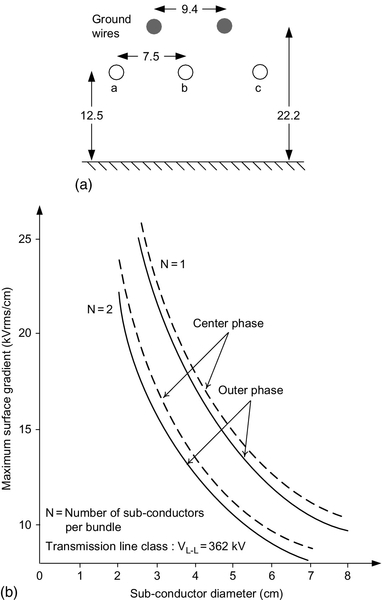
A Vrated = 345 kVL–L transmission line with go = 21.1 kV/cm (e.g., see Fig. E8.4.1b), r = 1.6 cm, d = 760 cm, m = 0.84 where at an altitude of 6000 feet the barometric pressure is 23.98 inches Hg (mercury) results at a temperature of −30°F in an air density factor of δ = 1.00. Calculate the critical disruptive voltage VL–N_o.
Solution to Application Example 8.4
The critical disruptive voltage is VL–N_o = 174 kV. That is, (VL–N_o ·![]() ) = 300 kVL–L < Vrated and corona will exist on this 345 kV line—even under fair weather conditions. Under foul (e.g., dirt, rain, frost) weather conditions the critical value of 300 kVL–L will be further reduced. Figure E8.4.1a gives the transmission line dimensions in meters for the VL–L = 362 kV class. Figure E8.4.1b presents the conductor surface gradient go for a 362 kV class of transmission lines. N is the number of phase (sub) conductors. Similar plots are given in [47] for other classes of transmission lines, e.g., aluminum-cable steel reinforced (ACSR).
) = 300 kVL–L < Vrated and corona will exist on this 345 kV line—even under fair weather conditions. Under foul (e.g., dirt, rain, frost) weather conditions the critical value of 300 kVL–L will be further reduced. Figure E8.4.1a gives the transmission line dimensions in meters for the VL–L = 362 kV class. Figure E8.4.1b presents the conductor surface gradient go for a 362 kV class of transmission lines. N is the number of phase (sub) conductors. Similar plots are given in [47] for other classes of transmission lines, e.g., aluminum-cable steel reinforced (ACSR).
The power loss associated with corona can be represented by shunt conductance. Figure E8.4.2 presents the coronal loss during fair weather conditions for different types of transmission lines. Corona loss ranges from about 0 up to 35 kW per three-phase mile. For a 500 mile transmission line the latter loss per mile value amounts to 17.5 MW. At line-to-line voltages above 230 kV, it is preferable to use more than one conductor per phase, which is known as bundling of conductors. The bundle can consist of two, three, four, or more subconductors. Figure E8.4.3 illustrates a flat configuration consisting of three bundles with six subconductors each. Bundling increases the effective radius of the line’s conductor per phase and reduces the electric field strength ![]() near the conductors, which reduces corona power loss, audible noise, radio and television interference, and the generation of ozone (O3) and nitrogen oxides (NOx). Another important advantage of bundling is reduced transmission line reactance, therefore increasing transmission capacity. Table E8.4.1 illustrates bundle dimensions as a function of the number of subconductors.
near the conductors, which reduces corona power loss, audible noise, radio and television interference, and the generation of ozone (O3) and nitrogen oxides (NOx). Another important advantage of bundling is reduced transmission line reactance, therefore increasing transmission capacity. Table E8.4.1 illustrates bundle dimensions as a function of the number of subconductors.

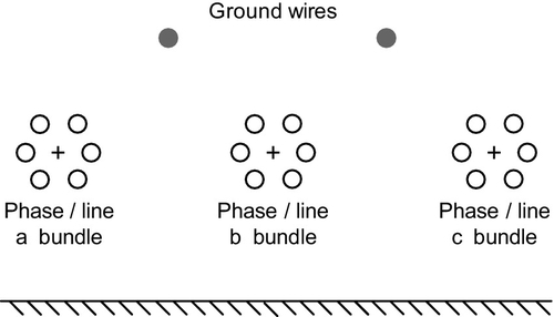
Table E8.4.1
Bundle Diameters as a Function of Number of Subconductors
| Conductors per phase | Bundle diameter (cm) |
| 2 | 45.7 |
| 3 | 52.8 |
| 4 | 64.6 |
| 6 | 91.4 |
| 8 | 101.6 |
| 12 | 127.0 |
| 16 | 152.4 |
8.2.4.8 Negative Effects of EMFs [50,51] and Corona
Biological Effects of Electric Fields  on People and Animals
To date, no specific biological effect of AC electric fields of the type and value applicable to transmission lines has been conclusively found and accepted by the scientific community. It is noteworthy to mention the rules established in the USSR (Union of Soviet Socialist Republics) for extrahigh voltage (EHV) substations and EHV transmission lines. For substations, limits for the duration of work in a day have been established as indicated in Table 8.1.
Table 8.1
Union of Soviet Socialist Republics (USSR) Rules for Duration of Work in Substations
| Electric field strength | Permissible duration (minutes per day) |
| < 5 | No restriction |
| 5-10 | 180 |
| 10-15 | 90 |
| 15-20 | 10 |
| 20-25 | 5 |
For transmission lines, considering the infrequent and nonsystematic exposure, higher values of the electric field strength |![]() | are accepted:
| are accepted:
• 20 kV/m for difficult terrain,
• 15–20 kV/m for nonpopulated region, and
• 10–12 kV/m for road crossing.
Suggested Biological Effects of Magnetic Fields  and
and  on People and Animals
The value of the magnetic field strength ![]() at ground level close to transmission lines is of the order of 5–14 A/m corresponding to magnetic field densities of |
at ground level close to transmission lines is of the order of 5–14 A/m corresponding to magnetic field densities of |![]() | from 0.08 to 0.3 G. Note that 1 gauss (G) is equivalent to 10–4 tesla (T) or 10–4 Wb/m2 or 10–4 Vs/m2 in the meter-kilogram-second-ampere (MKSA) system of units.
| from 0.08 to 0.3 G. Note that 1 gauss (G) is equivalent to 10–4 tesla (T) or 10–4 Wb/m2 or 10–4 Vs/m2 in the meter-kilogram-second-ampere (MKSA) system of units.
Magnetic AC fields have been reported to affect blood composition, growth, behavior, immune systems, and neural functions. However, at present, there is a lack of conclusive evidence.
Effects of Corona
Corona produces in the range of VL–L = 230 kV and higher
• audible (acoustic) hissing sound in the vicinity of the transmission corridor,
• ozone (O3) and NOx, where NOx is a generic term for the mono-nitrogen oxides NO and NO2 (nitric oxide and nitrogen dioxide), and
• radio and television interference.
The audible noise is an environmental concern. Radio interference (RI) occurs in the AM (amplitude modulation) band. Rain and snow may produce moderate TV interference (TVI) in a low signal area. Note that voice signals are frequency modulated (FM), and video signals are amplitude modulated (AM). More recently high-definition television (HDTV) relies on digital signals which are less impacted by corona.
8.2.4.9 Solutions for the Minimization of EMFs, Corona, and Other Environmental Concerns in Newly Designed Transmission Lines
Designing a transmission line with minimum environmental impact requires a study of five key factors:
1. impact of electric ![]() and magnetic fields
and magnetic fields ![]() ,
,
2. visual impact of the design,
3. generation of corona and its influence on radio and television interference,
4. air pollution via the generation of ozone O3 and NOx, and
5. impact of physical location.
A properly designed transmission line will have almost no perceptible negative environmental effects during fair weather, thus reducing disturbances, if they occur at all, to a small fraction of time.
EMFs
Although electric fields can be more readily reduced by shielding through structures with high conductivity (e.g., fences, trees), the reduction of magnetic fields is more difficult to achieve through shields with high permeability. Compensation or canceling of magnetic fields through the suspension of several transmission-line systems (e.g., reverse-phased double circuits) on the same tower as well as mounting the lines on higher towers near populated areas are frequently employed solutions. The employment of higher transmission-line voltages increases electric fields; however, they reduce the magnetic fields, which are more difficult to deal with.
Visual Impact
Reduction of the visual impact of a transmission line requires proper blending of the line with the countryside. Also the design and the location of supporting structures should not be objectionable to observers. Improvement in visual impact must be evaluated in conjunction with the economic penalty that the design incurs.
Audible Noise, Radio Interference (RI), and Television Interference (TVI) Caused by Corona
In the United States, there exist no regulations on a local or federal level that expressly limit the level of radio noise that a transmission line may produce. The Federal Communications Commission (FCC) places power transmission lines in the category of “incidental radiation device”. As such, the FCC requires that the “device shall be operated so that the radio frequency energy that is emitted does not cause any emissions, radiation or induction which endangers the function of a radio navigation service or other safety services, or seriously degrades, obstructs or repeatedly interrupts a radio communication service” operating in accordance with FCC regulations. Figure 8.10 shows typical frequency spectra of corona-induced radio noise, and Figure 8.11 illustrates a typical lateral profile of radio noise. Figure 8.12 illustrates radio noise tolerability criteria caused by corona, one for fair weather and one for foul weather; in addition there exists a 120 Hz hum (at 60Hz) due to the changing energy content of the lines. Video signals are more affected than sound signals because they are amplitude modulated whereas the latter are frequency modulated. HDTV is less affected by corona. A reduction of the radio noise entails a reduction of corona effects (e.g., bundle conductors). Note that the number of decibels (dB) is defined by dB = 20log10(vout/vin).


Ozone (O3) and NOx Generation
NOx is a generic term for the mono-nitrogen oxides NO and NO2 (nitric oxide and nitrogen dioxide). Figure 8.13 shows an example of ozone recordings for a 1300 kV line with large corona loss of 650 kW/km. Although ozone is the primary gaseous corona product, nitrogen oxides (NOx) may also be generated. The percentage of nitrogen oxide production is about one-sixth of that of ozone. The generation of ozone due to disassociation of oxygen in the corona region around the conductor is not of sufficient magnitude to be harmful. At ground level it has been found to be less than the daily natural variation. Conductor bundling is one method of reducing corona and its associated ozone generation.

Impact of Physical Location of Transmission Lines
The designer must also consider the environmental effects that the transmission line will have by its presence on certain land. These include the effect on wildlife, use of park areas, access to property, future planning, land values, and existing electromagnetic signal sources (e.g., communication transmitters). This is accomplished by rating each land parcel and selecting a route with a minimum environmental impact.
8.2.4.10 Economic Considerations
Corona loss of a well-designed transmission line should be below 1 kW per three-phase mile. This loss can be controlled by selecting proper configurations of bundle conductors (see Fig. E8.4.3 and Table E8.4.1). A bundle conductor is a conductor made up of two or more subconductors, and is used as one-phase conductor. Bundle conductors are not economical at or below 200 kV, but for rated voltages of 400 kV or more they are the best solution for overhead transmission lines. The increase in transmitting capacity justifies economically the use of two-conductor bundles on 220 kV lines.
The advantages of bundle conductors are higher disruptive voltage with conductors of reasonable dimensions, reduced surge impedance and consequent higher power capabilities, and less rapid increase of corona loss and RI with increased voltage. These advantages must be weighed against increased circuit cost and increased charging apparent power (kVA). Theoretically there is an optimum subconductor separation for bundle conductors that will give the minimum crest gradient on the surface of a subconductor and hence highest disruptive voltage.
8.2.4.11 No-Cost/Low-Cost EMF Mitigation Hearings of PUC of California [52]
Electric fields ![]() measured in V/m are created whenever power lines are energized with a voltage, whereas magnetic fields
measured in V/m are created whenever power lines are energized with a voltage, whereas magnetic fields ![]() measured in A/m (or
measured in A/m (or ![]() measured in milligauss) are created when current flows through the lines. Both electric and magnetic fields attenuate rapidly with distance from the source. Electric fields are effectively shielded by materials such as trees or buildings, whereas magnetic fields are not easily shielded by objects or materials. Therefore, concerns regarding potential power line EMF health effects arise primarily due to exposure to magnetic fields
measured in milligauss) are created when current flows through the lines. Both electric and magnetic fields attenuate rapidly with distance from the source. Electric fields are effectively shielded by materials such as trees or buildings, whereas magnetic fields are not easily shielded by objects or materials. Therefore, concerns regarding potential power line EMF health effects arise primarily due to exposure to magnetic fields ![]()
On January 15, 1991, the California Public Utilities Commission (CPUC) began an investigation to consider the Commission’s potential role in mitigating health effects, if any, of EMFs created by
1. electric utility power lines, and
2. cellular radiotelephone facilities.
Due to the lack of scientific or medical conclusions about potential health effects from utility electric facilities and power lines, the CPUC adopted seven interim measures that help to address public concern on this subject.
• No-cost and low-cost steps to reduce EMF levels: When regulated utilities design new projects or upgrade existing facilities, approximately 4% of the project’s budget may be used for reducing EMFs. The CPUC did not set specific reduction levels for EMFs. It was considered to be inappropriate to set a specific numerical standard until a scientific basis for doing so exists. No-cost measures are those steps taken in the design stage, including changes in standard practice, that will not increase the project cost but will reduce the magnetic flux density. Maximum (worst case) magnetic flux densities that could be permitted are ranging from 1 to 10 mG. Low-cost measures are those steps that will cost about 4% or less of the total project cost and will reduce the magnetic field flux density in an area (e.g., by a school, near residence) by approximately 15% or more at the edge of the right-of-way.
• New designs to reduce EMF levels: The CPUC initiated workshops to establish guidelines for new and rebuilt facilities. These guidelines incorporate alternative sites, increase the size of rights-of-way, place facilities underground, and use other suggested methods for reducing EMF levels at transmission, distribution, and substation facilities.
• Uniform residential and workplace EMF measurement methods are to be established.
• Promotion of education and research: The Department of Health Services (DHS) should manage such programs supported by public and utility funds.
CPUC-regulated utilities and municipal utilities may use ratepayer funds to pay their share of development costs for the following programs:
• EMF research, and
• other research.
It has been many years since the CPUC devised the above-mentioned seven interim measures. During this time a significant body of scientific research has developed. In 2002 the DHS completed its comprehensive evaluation of existing scientific studies. Although there is still no consensus in the scientific community regarding health risks of EMF exposure, DHS reported troubling indications that EMF exposure may increase risk of certain diseases (e.g., childhood and to some extent adult leukemia, adult brain cancer, Lou Gehrig’s disease) and other health problems.
8.2.4.12 Summary and Conclusions
The results of the many papers and books published in the area of generation of EMFs and corona by transmission lines can be summarized as follows:
• Transmission lines with line-to-line voltages of up to 200 kV do not generate any significant amount of corona; however, such lines can generate significant amounts of EMFs. For transmission lines with line-to-line voltages above 200 kV the following conclusions can be drawn: Maximum (worst case) AC electric field strength ![]() at ground level below transmission line is up to |
at ground level below transmission line is up to |![]() | = 15 V/mm at a line-to-line voltage of 1050 kV. The maximum occurs at the edge of transmission corridor. An electric field strength of |
| = 15 V/mm at a line-to-line voltage of 1050 kV. The maximum occurs at the edge of transmission corridor. An electric field strength of |![]() | = 5 V/mm is acceptable. Maximum (worst case) AC magnetic field strength
| = 5 V/mm is acceptable. Maximum (worst case) AC magnetic field strength ![]() at ground level below transmission line is |
at ground level below transmission line is |![]() | = 14 A/m corresponding to a maximum flux density |
| = 14 A/m corresponding to a maximum flux density |![]() | = 0.176 G = 176 mG at a phase current of 2000 A. Note the DC earth field is about Bearth = 0.5 G. A flux density of |
| = 0.176 G = 176 mG at a phase current of 2000 A. Note the DC earth field is about Bearth = 0.5 G. A flux density of |![]() | = 3 mG is acceptable.
| = 3 mG is acceptable.
• Corona depends on construction of transmission towers including type of conductors, e.g., hollow copper cable (e.g., HH) or aluminum cable steel reinforced (ACSR), surface of cable, type of bundle, fair or foul weather conditions, temperature, barometric pressure, and air density.
• Corona loss of 1 kW/three-phase mile is acceptable.
• Radio and television interference occurs within the 0.1 MHz to 1 GHz range.
• Audible noise ranges from 50 Hz to 120 Hz (power-frequency hum) to 10 kHz (hissing noise).
• Additional ozone (O3) production is in the range of 15 ppb (parts per billion). The naturally occurring level is 25 ppb. That is, O3 production by power lines is insignificant.
• Nitrogen oxide (NOx) production is about one-sixth of the ozone generation. That is, NOx production by power lines is insignificant.
• Active compensation (e.g., through compensation of EMFs by arranging several transmission systems on one tower, by reducing, compensating, or canceling EMFs in houses through compensation circuits) is possible.
• Passive (e.g., horizontal or vertical mesh structures, conductive suits) and natural shielding (e.g., trees, houses) is possible.
• Overall control of EMFs and corona through transmission line (e.g., bundle conductors, reverse-phased double circuit) and tower construction (e.g., height) is feasible; it is, however, more expensive.
• For newly designed transmission lines all environmental concerns (e.g., limits for EMFs, RI, and TVI) and technical constraints (corona loss of 1 kW/three-phase mile) can be satisfied.
• The mitigation of detrimental environmental, technical, or economic effects of existing transmission lines will be difficult to achieve at no or low cost as proposed by the Public Utilities Commission of California.
• The issue has surfaced that corona on transmission lines may create X-rays. A practical lower bound of X-rays is at least 2 keV. However, the electrical discharges of coronal activity on transmission lines can produce electron energies on the order of about 1–10 eV. This is sufficient for production of visible light but is orders of magnitude below electron energies necessary for the production of X-rays by transmission line corona [53]. That is, transmission lines do not generate X-rays.
8.2.5 Distributed-, Cogeneration, and Frequency/Voltage Control
Renewable energy sources such as solar and windpower [54,55] plants have an intermittent power output. Nevertheless it is desirable to operate them at maximum power output, for example, employment of peak-power tracker for photovoltaic plant [56]. With such peak-power and intermittent-power constraints it is impossible to operate a power system with distributed generation (DG) sources only because the drooping characteristics [57] which are responsible for load sharing require that at least one plant can deliver the additional power as requested by the utility customers, thus serving as base-load plant with spinning reserve capability. This is the reason why in Denmark [58] the control of the power system becomes more difficult as the renewable contribution approaches 50% of the total generation. This is so because the entire system exhibits properties of so-called weak systems with low short-circuit capabilities. As an alternative to a large power plant serving as a frequency leader—which can deliver sufficient additional power so that the frequency control will not be impaired—it is possible to strategically place storage peak-power plants based on pumped-hydro [59,60] or compressed-air facilities [61,62] that can provide peak power for several hours per day, for example, 22 h of continuous generation at 1600 MW.
Related to the availability of spinning reserve—which should be in the neighborhood of about 5–10% of the total installed power capacity—is the fast valving [63,64] so that the time constants of the speed control circuit (e.g., governor) can be maintained within certain limits. In addition near-term [65,66] and long-term [67,68] load forecasts are important for the reliable operation of the power system with intermittently operating renewable energy sources. It is the task of control and dispatch centers to set the load reference points for each and every generation plant within an interconnected power system. From the following application examples one learns that renewable energy sources alone—operated at their maximum-power points [56]—cannot maintain frequency and voltage control. This is so because there must be a spinning reserve of power generation and sufficient facilities to control reactive power.
8.2.5.1 Application Example 8.5: Frequency Control of an Interconnected Power System Broken into Two Areas: The First One with a 300 MW Coal-Fired Plant and the Other One with a 5 MW Wind-Power Plant
Figure P4.12 of Chapter 4 shows the block diagram of two generating plants interconnected by a tie line (transmission line).
Data for generation set #1 (steam turbine and generator) are as follows:
Angular frequency change (Δω1) per change in generator output power (ΔΡ1) having the droop characteristic of ![]() = 0.01 pu, load change (ΔPL1) per frequency change (Δω1) resulting in
= 0.01 pu, load change (ΔPL1) per frequency change (Δω1) resulting in ![]() = 0.8 pu, step load change
= 0.8 pu, step load change ![]() angular momentum of steam turbine and generator set M1 = 4.5, base apparent power Sbase = 500 MVA, governor time constant TG1 = 0.01 s, valve changing (charging) time constant TCH1 = 0.5 s, and (load reference set point)1 = 0.8 pu.
angular momentum of steam turbine and generator set M1 = 4.5, base apparent power Sbase = 500 MVA, governor time constant TG1 = 0.01 s, valve changing (charging) time constant TCH1 = 0.5 s, and (load reference set point)1 = 0.8 pu.
Data for generation set #2 (wind turbine and generator) are as follows:
Frequency change (Δω2) per change in generator output power (ΔP2) having the droop characteristic ![]() = 0.02 pu, load change (ΔPL2) per frequency change (Δω2) resulting in
= 0.02 pu, load change (ΔPL2) per frequency change (Δω2) resulting in ![]() = 1.0 pu, step load change
= 1.0 pu, step load change ![]() pu =
pu = ![]() pu, angular momentum of wind turbine and generator set M2 = 6, base apparent power Sbase = 500 MVA, governor time constant TG2 = 0.02 s, valve (blade control) changing (charging) time constant TCH2 = 0.75 s, and (load reference set point)2 = 0.8 pu.
pu, angular momentum of wind turbine and generator set M2 = 6, base apparent power Sbase = 500 MVA, governor time constant TG2 = 0.02 s, valve (blade control) changing (charging) time constant TCH2 = 0.75 s, and (load reference set point)2 = 0.8 pu.
Data for tie line: ![]() with Xtie = 0.2 pu.
with Xtie = 0.2 pu.
a) List the ordinary differential equations and the algebraic equations of the block diagram of Fig. P4.12 of Chapter 4.
b) Use either Mathematica or MATLAB to establish transient and steady-state conditions by imposing a step function for load reference set point (s)1 = ![]() pu, load reference set point (s)2 =
pu, load reference set point (s)2 = ![]() pu, and run the program with zero step load changes ΔΡL1 = 0, ΔΡL2 = 0 for 5 s. After 5 s impose the positive step-load change ΔΡL1(s) =
pu, and run the program with zero step load changes ΔΡL1 = 0, ΔΡL2 = 0 for 5 s. After 5 s impose the positive step-load change ΔΡL1(s) = ![]() pu =
pu =![]() pu, and after 7 s impose the negative step-load change ΔΡL2(s) =
pu, and after 7 s impose the negative step-load change ΔΡL2(s) = ![]() pu =
pu =![]() pu, for the droop characteristics R1 = 0.01 pu and R2 = 0.02 pu to find the transient and steady-state responses Δω1(t) and Δω2(t).
pu, for the droop characteristics R1 = 0.01 pu and R2 = 0.02 pu to find the transient and steady-state responses Δω1(t) and Δω2(t).
c) Use either Mathematica or MATLAB to establish transient and steady-state conditions by imposing a step function for load reference set point ![]() load reference set point
load reference set point ![]() and run the program with zero step load changes ΔΡL1 = 0, ΔΡL2 = 0 for 5 s. After 5 s impose positive step-load change ΔΡL1(s) =
and run the program with zero step load changes ΔΡL1 = 0, ΔΡL2 = 0 for 5 s. After 5 s impose positive step-load change ΔΡL1(s) = ![]() pu =
pu =![]() pu, and after 7 s impose the negative step-load change ΔΡL2(s) =
pu, and after 7 s impose the negative step-load change ΔΡL2(s) = ![]() pu =
pu =![]() pu, for the droop characteristics R1 = 0.01 pu (coal-fired plant) and R2 = 0.5 pu (wind-power plant) to find the transient and steady-state responses Δω1(t) and Δω2(t).
pu, for the droop characteristics R1 = 0.01 pu (coal-fired plant) and R2 = 0.5 pu (wind-power plant) to find the transient and steady-state responses Δω1(t) and Δω2(t).
Solution to Application Example 8.5
a) List of ordinary differential equations


There are 11 independent equations and 11 unknowns. The latter are ɛ11, ΔPvalve1, ΔPmech1, ɛ21, ΔPtie, Δω1, ɛ12, ΔPvalve2, ΔPmech2, ɛ22, Δω2.
b) and c) The Mathematica program and the MATLAB program codes are presented in Table E8.5.1 and Table E8.5.2, repectively.
Table E8.5.1
Mathematica program list for Application Example 8.5
| Remove [Dw1, R1, Loadref1, E11, DPvalve1, DPmech1, DPl1, E12, Tg1, Tch1, M1, D1, Dw2, R2, Loadref 2, E22, DPvalve2, DPmech2, DPl2, E21, Tch2, M2, D2, Sbase, eq1, eq2, eq3, ic1, ic2, ic3, DPtie, E3, Tie, Xtie, ic4, ic5, ic6, ic7]; Sbase=500000000; M1=4.5; Tg1=0.01; Tch1=0.5; R1=0.01; D1=0.8; M2=6; Tg2=0.02; Tch2=0.75; R2=0.02; D2=1.0; Xtie=0.2; Tie=377/Xtie; Loadref 1 [t_]:=If [t<0,0,0.8]; Loadref 2 [t_]:=If [t<0,0,0.8]; DPl1 [t_]:=If [t<5,0,0.2]; DPl2 [t_]:=If [t<7,0,–0.2]; ic1=Dw1[0]= = 0; ic2=DPmech1[0]= = 0; ic3=DPvalve1[0]= = 0; ic5=Dw2[0]= = 0; ic6=DPmech2[0]= = 0; ic7=DPvalve2[0]= = 0; ic4=DPtie [0]= = 0; E11[t_]:=Loadref1[t]–(Dw1[t]/R1); E12[t_]:=DPmech1[t]–(DP11[t]-DPtie[t]); E3[t_]:=Dw1[t]–Dw2[t]; E22 [t_]:=Loadref2[t]–(Dw2[t]/R2); E21[t_]:=DPmech2[t]–(DPl2[t]+DPtie [t]); eq1=Dw1’[t]= =(1/M1)*(E12[t]–D1*Dw1[t]); eq2=DPmech1’[t]= =(1/Tch1)*(DPvalve1[t]–DPmech1[t]); eq3=DPvalve1’[t]= =(1/Tg1)*(E11[t]–DPvalve1[t]); eq5=Dw2’[t]= =(1/M2)*(E21[t]–D2*Dw2[t]); eq6=DPmech2’[t]= =(1/Tch2)*(DPvalve2[t]–DPmech2 [t]); eq7 = DPvalve2’[t]= =(1/Tg2)*(E22[t]–DPvalve2[t]); eq4=DPtie’[t]= = Tie*E3[t]; sol=NDSolve [{eq1,eq2,eq3, eq4,eq5,eq6,eq7,ic1,ic2,ic3,ic4,ic5,ic6,ic7}, {DW1 [t],DPmech1 [t],DPvalve1 [t],DPtie[t], Dw2[t],DPmech2[t], DPvalve2 [t]}, {t,0,100},MaxSteps–>1000000]; Plot [Dw1[t]/sol,{t,0,100}, PlotRange–> All, AxesLabel–>{“t”, “Dw1(t)[pu]”}] Plot [Dw2 [t]/sol,{t,0,100}, PlotRange–>All, AxesLabel–>{“t”, “Dw2(t)[pu]”}] |

Table E8.5.2
MATLAB program list for Application Example 8.5
| %defining the input Sbase=500e6; M1=4.5; Tg1=0.01; Tch1=0.5; R1=0.01; D1=0.8; M2=6; Tg2=0.02; Tch2=0.75; R2=0.02; D2=1; Xtie=0.2; Tie=377/Xtie; %time span T1=0:0.001:20; T=T1.’; %solving system of equations opts=odeset(‘AbsTol’,1e–11,’RelTol’,1e–7; [t0,x0]=ode45)@F2,T, [0;0;0;0;0;0;0],o pts,M1,Tg1,Tch1,R1,D1,M2,Tg2,Tch2,R2, D2,Tie); %plot results figure; Plot(t0,x0(:;4)); Grid on, zoom on; Title(,Transient response of Delta omega1(t) vs t’)); xlabel(‘t’); ylabel(‘Deltaomega1(t)’); figure; Plot (t0,x0 (:;1)); Grid on, zoom on; Title (‚Transient response of Delta omega2 (t) vs t′)); xlabel (‘t’); ylabel (‘Deltaomega2(t)’); where the function F2 is: function xprime=F2 (t,x,M1,Tg1,Tch1, R1,D1,M2,Tg2,Tch2,R2,D2,Tie); if t<5; DPl1=0; elseDPl1=0.2; end if t<7; DPl2=0; elseDPl2=–0.2; end if t<0; load1=0; else load1=0.8; end if t<0; load2=0; else load2=0.8; end xprime=zeros(7,1); xprime(1)=(1/M1)*(x(2)–DPl1–x(7)–(D1*x(1))); xprime(2)=(1/Tch1)*(x(3)–x(2); xprime(3)=(1/Tg1)*(load1–(x(1))*(1/R1)–x(3))); xprime(4)=(1/M2)*(x(5)–DPl2–x(7)–(D2*x(4))); xprime(5)=(1/Tch2)*(x(6)–x(5); xprime(6)=(1/Tg2)*(load2-(x(4))*(1/R2)-x(6))); xprime(7)=(Tie)*(x(12)-x(4)); |

The angular frequency deviations Δω1(t) and Δω2(t) based on Mathematica for droop characteristics with R1 = 0.01 pu, R2 = 0.02 pu are shown in Figs. E8.5.1 and E8.5.2. Note that there is instability, and both plots result in the same frequency response.


The angular frequency deviations Δω1(t) and Δω2(t) based on Mathematica for droop characteristics with R1 = 0.01, R2 = 0.5 are shown in Figs. E8.5.3 and E8.5.4. Note that there is stability, and both plots result in the same frequency response.


The angular frequency deviations Δω1(t) and Δω2(t) based on MATLAB for droop characteristics with R1 = 0.01 pu, R2 = 0.02 pu are shown in Figs. E8.5.5 and E8.5.6 confirming the results of Figs. E8.5.1 and E8.5.2.


The angular frequency deviations Δω1(t) and Δω2(t) based on MATLAB for droop characteristics with R1 = 0.01 pu, R2 = 0.5 pu are shown in Figs. E8.5.7 and E8.5.8 confirming the results of Figs. E8.5.3 and E8.5.4.


8.2.5.2 Application Example 8.6: Frequency Control of an Interconnected Power System Broken into Two Areas: The First One with a 5 MW Wind-Power Plant and the Other One with a 5 MW Photovoltaic Plant
Figure P4.12 of Chapter 4 shows the block diagram of two generators interconnected by a tie line (transmission line).
Data for generation set #1 (wind turbine and generator) as follows:
Frequency change (Δω1) per change in generator output power (ΔΡ1) having the droop characteristic ![]() load change (ΔPL1) per frequency change (Δω1) yields
load change (ΔPL1) per frequency change (Δω1) yields ![]() = 0.8pu, step-load change ΔΡL1(s) =
= 0.8pu, step-load change ΔΡL1(s) = ![]() pu =
pu = ![]() pu, angular momentum of wind turbine and generator set M1 = 4.5, base apparent power Sbase = 50 MVA, governor time constant TG1 = 0.01 s, valve (blade control) changing (charging) time constant TCH1 = 0.1 s, and (load reference set point)1 = 0.8 pu.
pu, angular momentum of wind turbine and generator set M1 = 4.5, base apparent power Sbase = 50 MVA, governor time constant TG1 = 0.01 s, valve (blade control) changing (charging) time constant TCH1 = 0.1 s, and (load reference set point)1 = 0.8 pu.
Data for generation set #2 (photovoltaic array and inverter):
Frequency change (Δω2) per change in inverter output power (ΔΡ2) having the droop characteristic ![]() load change (ΔPL2) per frequency change (Δω2) yields D2 =
load change (ΔPL2) per frequency change (Δω2) yields D2 = ![]() = 1.0 pu, step-load change ΔΡL2(s) =
= 1.0 pu, step-load change ΔΡL2(s) = ![]() pu =
pu =![]() pu, equivalent angular momentum M2 = 6, base apparent power Sbase = 50 MVA, governor time constant TG2 = 0.02 s, equivalent valve changing (charging) time constant TCH2 = 0.1 s, and (load reference set point)2 = 0.8 pu.
pu, equivalent angular momentum M2 = 6, base apparent power Sbase = 50 MVA, governor time constant TG2 = 0.02 s, equivalent valve changing (charging) time constant TCH2 = 0.1 s, and (load reference set point)2 = 0.8 pu.
Data for tie line: ![]() with Xtie = 0.2pu.
with Xtie = 0.2pu.
Use either Mathematica or MATLAB to establish transient and steady-state conditions by imposing a step function for load reference set point(s)1 = ![]() pu, load reference set point(s)2 =
pu, load reference set point(s)2 = ![]() pu and run the program with a zero step load changes ΔPL1 = 0, ΔPL2 = 0 for 5 s. After 5 s impose step-load change ΔΡL1(s) =
pu and run the program with a zero step load changes ΔPL1 = 0, ΔPL2 = 0 for 5 s. After 5 s impose step-load change ΔΡL1(s) = ![]() pu =
pu =![]() pu, and after 7 s impose the step-load change ΔΡL2(s) =
pu, and after 7 s impose the step-load change ΔΡL2(s) = ![]() pu =
pu =![]() pu, to find the transient and steady-state responses Δω1(t) and Δω2(t).
pu, to find the transient and steady-state responses Δω1(t) and Δω2(t).
Solution to Application Example 8.6
The Mathematica program is presented in Table E8.6.1 and the resulting plots are shown in Figs. E8.6.1 and E8.6.2.
Table E8.6.1
Mathematica program list for Application Example 8.6
| Remove[Dw1, R1, Loadref1, E11,DPvalve1, DPmech1, DPl1, E12,Tg1,Tch1, M1, D1, Dw2, R2, Loadref2, E22, DPvalve2, DPmech2, DPl2, E21, Tch2,M2, D2, Sbase, eq1, eq2, eq3, ic1, ic2, ic3, DPtie, E3, Tie, Xtie, ic4, ic5, ic6, ic7]; Sbase=500000000; M1=4.5; Tg1=0.01; Tch1=0.1; R1=0.5; D1=0.8; M2=6; Tg2=0.02; Tch2=0.1; R2=0.5; D2=1.0; Xtie=0.2; Tie=377/Xtie; Loadref1[t_]:=If[t<0,0,0.8]; Loadref2[t_]:=If[t<0,0,0.8]; DPl1[t_]:=If[t<5,0,0.1]; DPl2[t_]:=If[t<7,0,-0.1]; ic1=Dw1[0]==0; ic2=DPmech1[0]==0; ic3=DPvalve1[0]==0; ic5=Dw2[0]==0; ic6=DPmech2[0]==0; ic7=DPvalve2[0]==0; ic4=DPtie[0]==0; E11[t_]:=Loadref1[t]-Dw1[t]/R1; E12[t_]:=DPmech1[t]-(DPl1[t]-DPtie[t]); E3[t_]:=Dw1[t]-Dw2[t]; E22[t_]:=Loadref2[t]-(Dw2[t]/R2); E21[t_]:=DPmech2[t]-(DPl2[t]+DPtie[t]); eq1=Dw1'[t]==(1/M1)*(E12[t]-D1*Dw1[t]); eq2=DPmech1'[t]==(1/Tch1)*(DPvalve1[t]-DPmech1[t]); eq3=DPvalve1'[t]==(1/Tg1)*(E11[t]-DPvalve1[t]); eq5=Dw2'[t]==(1/M2)*(E21[t]-D2*Dw2[t]); eq6=DPmech2'[t]==(1/Tch2)*(DPvalve2[t]-DPmech2[t]); eq7=DPvalve2'[t]==(1/Tg2)*(E22[t]-DPvalve2[t]); eq4=DPtie'[t]==Tie*E3[t]; sol=NDSolve[{eq1,eq2,eq3,eq4,eq5,eq6,eq7,ic1, ic2,ic3,ic4,ic5,ic6,ic7},{Dw1[t],DPmech1[t], DPvalve1[t],DPtie[t],Dw2[t],DPmech2[t], DPvalve2[t]},{t,0,100},MaxSteps->1000000]; Plot[Dw1[t]/.sol[[1]],{t,0,100},PlotRange-> All,AxesLabel->{"t[s]","Dw1[t][pu]"}] Plot[Dw2[t]/.sol[[1]],{t,0,100},PlotRange-> All,AxesLabel->{"t[s]","Dw2[t][pu]"}] |


The angular frequency deviations Δω1(t) and Δω2(t) for droop characteristics with R1 = 0.5 pu, R2 = 0.5 pu are much larger than those in Application Example 8.5, that is, there is instability. See Problems 8.5 through 8.7.
From Application Examples 8.5 and 8.6 one draws the following conclusions:
1. Renewable energy sources stemming from solar and wind are likely to be operated at their maximum output power. This requires that the slope R of the drooping characteristic of a renewable power source is large as is depicted in Figs. 8.14 and 8.15. As a consequence of the large R, the change in output of the renewable source results in instability or a large frequency change Δω.


2. Solar, wind, and tidal power sources are intermittent in nature and their output power cannot be controlled by the dispatch center of a utility system.
3. Due to issues 1 and 2 distributed generation (DG) based on solar and wind power is not possible unless either a base load plant (e.g., gas- or coal-fired plant) or a storage plant (e.g., pumped hydro, compressed air) is ready to deliver the additional power required. That is, the base load plant or the storage plant acts as a spinning reserve plant.
4. It has been discussed in Chapter 4 (Section 4.2.2.3) that an inverter requires a larger DC input voltage for capacitive/resistive load than for inductive/resistive operation. To utilize inverter components to their fullest unity power (about resistive operation) factor operation is preferred. This means a renewable power plant cannot be very effectively employed for reactive power or voltage control.
5. The governor time constant (e.g., TG1, TG2) and the valve changing (charging) time constant (e.g., TCH2, TCH2) must be small to guarantee stability. The latter time constant is fairly large for steam, hydro, and wind-power plants. This issue has been addressed in [63,64].
6. In summary it is not possible to operate a power system solely based on renewable power plants without storage plants because they do not easily lend themselves to frequency and voltage control.
8.3 Tools for detecting poor power quality
8.3.1 Sensors
To be able to detect power quality problems one must rely on voltage and current sensors such as low-inductive voltage dividers for voltage pickup, and low-inductive shunts and Hall sensors for current pickup. Components representing the interface between sensors and measuring instruments are potential and current transformers as well as optocouplers. Voltmeters, amperemeters, oscillographs, spectrum analyzers, and network analyzers are indispensable. Special power quality tools and selection guides have been developed for detecting power quality for single- and three-phase systems, such as power quality clamp meters, power quality analyzers, voltage event recorder systems, three-phase power loggers, series three-phase power quality loggers, three-phase power quality recorders, AC leakage current clamp meters, series three-phase power quality analyzers, high precision power analyzers, reliable power meters, multipoint power recorders, and other power quality-specific equipment. Some of them [69,70] are useful to analyze steady-state phenomena, and some of them are transient overvoltage/under-voltage meters recording outage time, deviation from rated voltage values (e.g., sags, swells), or the number of outages within a given time period, and an instrument that distinguishes the direction of the harmonic power flow as is described in the following application example.
8.3.2 Application Example 8.7: Detection of Harmonic Power Flow Direction at Point of Common Coupling (PCC)
IEEE Standard 519 [76] distinguishes between customer- and power system generated harmonics. If the current harmonics flowing from the power system to the customer are at the point of common coupling (PCC) within given limits [76] and the voltage harmonics at PCC are too large then the customer must install filters to prevent customer-generated current harmonics to enter the grid at PCC. In order to sense and measure customer-generated current harmonics design, a harmonic-current sensing equipment and a programmable filter so that the customer-generated current harmonics can be detected and controlled.
Solution to Application Example 8.7
The discrimination between the contributions of the customer and the power system to generated harmonic currents at PCC is based on Fig. E8.7.1 and [70–84]. Figure E8.7.1a represents the equivalent circuit of one customer connected to the power system at PCC indicated by the terminals A –Aʹ and B –Bʹ. To measure individual harmonic currents iA(h), iB(h) with respect to direction and amplitude a harmonic current sensing network (see Fig. E8.7.1b), which represents a programmable harmonic filter, is configured and connected by computer commands c1, c2, and c3 for a fraction of a second during which measurements take place. For measuring the current icustomer(h) the impedance and admittance ZPCCcustomer(h) and YPCC(h), respectively, will provide a short-circuit for icustomer(h)(t) during a fraction of a second, whereas the impedance ZPCCsystem(h) is blocking isystem(h)(t). For measuring the current isystem(h)(t) the impedance and admittance ZPCCsystem(h) and YPCC(h), respectively, will provide a short-circuit for isystem(h)(t) during a fraction of a second, whereas the impedance ZPCCcustomer(h) is blocking icustomer(h)(t). The harmonic impedance and admittance consists of inductors and capacitors whose very small losses—to achieve a high Q of the programmable filters—will be determined as described in [83]. Current and voltage sensors (e.g., Hall sensors [81] or low-inductive current shunts and voltage dividers [82] with optocouplers) will measure the direction of the harmonic power flow as detailed in [70–74].

The main advantages of this approach are
1. Nonintrusive measurements lasting a fraction of a second. Field tests can be executed in three steps, each step lasting less than 0.1 s. In the first step the harmonic current icustomer(h)(t) will be measured by configuring the programmable filter so that ZPCCcustomer(h) and YPCC(h) represent a short-circuit for a harmonic customer current of hth order, while ZPCCsystem(h) represents an open-circuit for the system harmonic current of hth order. In the second step ZPCCsystem(h) and YPCC(h) represent a short-circuit for the system harmonic current of hth order, while ZPCCcustomer(h) represents an open circuit for the system current of hth order. In the third step the total harmonic current will be measured when ZPCCcustomer(h) and ZPCCsystem(h) are bypassed and ![]() is an open circuit.
is an open circuit.
2. Real-time measurement while system operates under load.
3. No additional dissipation occurs.
4. Very small ohmic components of inductors and capacitors can be accurately determined [83], resulting in high Q of programmable harmonic filters.
5. In most harmonic standards [76,77] the harmonic current injection from the customer installation is limited. To enforce such limits by utilities these customer-injected harmonic currents at PCC icustomer(h)(t) must be reliably and accurately measured. This approach provides a tool for the utilities to measure customer harmonic currents. This will increase the reliability and efficiency of power system operation.
8.3.3 Maximum Error Analysis
The accurate online or real-time measurement of losses of circuit components such as transformers improves the reliability and security of a power system. Normally circuit components are equipped with temperature sensors (e.g., thermocouples, thermistors). This approach has two disadvantages.
1. Circuit components must be equipped with sensors during their construction, and off-the-shelf components cannot be used.
2. Temperature sensors provide information about the temperature at their location and not necessarily the temperature at the hot spot of an energy conversion device, and any temperature alarm may come too late to prevent an outage due to a fault.
The advantages of the real-time monitoring of losses of components (e.g., transformers) are that loss increases can be sensed or recorded at the time when a fault develops. In addition, the measurement components or instruments can be exchanged, thus minimizing the outage time of the transformer supplying the power system. Such a monitoring of the losses must rely on small maximum errors of the monitoring equipment.
Maximum error analysis has been extensively used in the past [70–73,85–87]. The online measurement of transformer losses under nonsinusoidal operation is discussed in detail in [87]. The real-time monitoring of iron-core and copper losses of single- and three-phase transformers is important, particularly for transformers feeding nonlinear loads. This section devises a new digital data-acquisition method for the separate online measurement of iron-core and copper losses of three-phase transformers under any full or partial load conditions. The accuracy requirements of the instruments employed (voltage and current sensors, volt and current meters) are addressed. The maximum errors are acceptably low if voltage and current sensors with 0.1 to 0.5% errors are used.
8.3.3.1 Review of Existing Methods
The separate online monitoring of the iron-core and copper losses of single- and three-phase transformers is desirable because additional losses due to power quality problems (e.g., harmonics, DC excitation) can be readily detected before any significant damage due to additional temperature rises occurs. Those losses can accurately and economically be measured for single-phase transformers via computer-aided testing (CAT) [71,88].
The known approaches for on-line loss measurement of high-efficiency transformers (e.g., efficiency greater than 97%) are inaccurate because they measure input and output powers and derive the loss from the difference of these two large values. The usually employed indirect method consisting of no-load (iron-core loss) and short-circuit (copper loss) tests [35] cannot be performed online while the transformer is partially or fully loaded. The same is valid for the loading back method [89].
Arri et al. presented an analog measurement circuit [90]. It is well known that there may occur zero-sequence currents on the Y-grounded side of a three-phase transformer, and these currents will produce corresponding losses in the transformer. The measuring circuit presented by Arri et al. cannot measure these zero-sequence components, and therefore the method is not suitable for transformers with grounding on any side (either primary or secondary). Moreover, Arri et al. rely on many instrument transformers (nine CTs and nine PTs) to convert the Δ connection to Y connection for a Y/Δ connected transformer: as a result the measuring accuracy is decreased. In [91] an analog measuring circuit with wattmeters is presented within a single-phase circuit.
This section presents a more accurate real-time method for digitally and separately measuring the steady-state iron-core and copper losses of three-phase transformers with various grounded connections while the transformers are operating at any load condition. This digital measuring circuit is based on voltage and current sensors (voltage dividers, shunts, PTs, CTs, or Hall devices), A/D converter, and personal computer. Using a computer-aided testing program (CATEA) [70] losses, efficiency, harmonics, derating, and wave shapes of all voltages and currents can be monitored within a fraction of a second.
The maximum measurement errors of the losses are acceptably small and vary in the range from 0.5 to 15%, mainly contingent on the accuracy of the voltage and current sensors used. Depending on the application, voltage dividers with optocouplers [73], current shunts with optocouplers, potential and current transformers (error < 0.1%), as well as Hall sensors [92] (error < 0.5%) can be employed.
When both voltage and current signals are obtained from Hall devices [92], the copper losses will include DC losses, if they exist. Provided voltage and current signals are generated by PT and CT sensors, the DC losses are not included in the copper losses, and must be measured by additional DC voltmeters and ammeters or sensors. In this case, the total loss consists of the iron-core, AC, and DC copper losses.
8.3.3.2 Approach
It is well known that for any Y (ungrounded) or Δ connected three-phase windings, the two-wattmeter method is often used to measure the power based on the voltages and currents of any two phases. For a Y grounded three-phase winding, an additional wattmeter is necessary for the voltage and current of the third phase, or those of the zero sequence. Therefore, for a transformer without grounding on any side (primary or secondary), power loss is measured with eight signals (voltages and currents of two phases for each side). If the primary or/and the secondary are grounded, the power loss can be measured with ten or twelve signals. This section deals with ten- and twelve-channel measuring circuits. The eight-channel measuring circuits for Y/Y ungrounded or Δ/Δ and Δ–Y ungrounded three-phase transformers are discussed in [73].
A ten-channel CAT circuit applied to Δ–Y0 (Y0 means Y grounded) connected three-phase transformers is shown in Fig. 8.16. The flowchart for the ten-channel signals is shown in Fig. 8.17. The output power (at the Y0 side) is

where ![]() and
and ![]() The transformer loss is
The transformer loss is


The loss component ![]() in Eq. 8-6 is included in the copper loss, which can be proved below:
in Eq. 8-6 is included in the copper loss, which can be proved below:

Note that the analog measuring circuit of [90] does not take into account zero-sequence components and, therefore, does not apply to general asymmetric operating conditions.
For Y–Y0 connected three-phase transformers (see Fig. 8.18), the output power can be written as

where ![]() . The transformer loss can be formulated as
. The transformer loss can be formulated as

where (![]() ) is included in the iron-core loss. This can be shown as follows:
) is included in the iron-core loss. This can be shown as follows:


For Y0–Y0 connected transformers, a twelve-channel circuit is used as shown in Fig. 8.19. The loss of the transformer can be derived directly from


The instantaneous expression pfe(t) in Eq. 8-10 includes two power components: the instantaneous iron-core loss and the instantaneous exciting reactive power. Similarly, pcu(t) in Eq. 8-7 includes the instantaneous copper loss and the instantaneous reactive power due to the leakage flux. At steady state, the average value of reactive power during one electric cycle is zero; therefore, the average values of pfe(t) and pcu(t) during one electric cycle reflect the steady-state iron-core and copper losses.
The instantaneous expressions of pfe(t) and pcu(t) of various three-phase transformer connections are listed in Table 8.2, where all current and voltage differences can be calibrated directly under either sinusoidal or nonsinusoidal conditions.
Table 8.2
Iron-Core and Copper Losses of Three-Phase Transformers
| pfe(t) | pcu(t) | |
| Y–Y (or Δ–Δ) | ||
| Δ–Y | ||
| Δ–Y0 | ||
| Y–Y0 | ||
| Y0–Y0 |
If the neutral line is disconnected, and v0′ and ib′ are not measured, Fig. 8.16 becomes the eight-channel loss-measuring circuit of Δ–Y connected three-phase transformers (Fig. 8.20), and the transformer loss is obtained from Eq. 8-6 with v0′= 0 [73]. Similarly, if the neutral line is disconnected, and i0′ and ![]() are not measured, Fig. 8.18 becomes the eight-channel loss-measuring circuit of Y–Y connected three-phase transformers, and the transformer loss is obtained from Eq. 8-9 with i0′= 0 [73]. The circuits valid for Δ–Y, Δ–Y0, and Y–Y0 connected transformers also apply for Y–Δ, Y0–Δ, and Y0–Y connected three-phase transformers, respectively. In these cases, the capital letters A, B, and C represent the secondary, and the lower case letters a, b, and c denote the primary. The corresponding iron-core and copper losses, listed in Table 8.2, are then negative. Table 8.3 shows valid methods for three-phase transformers of various connections.
are not measured, Fig. 8.18 becomes the eight-channel loss-measuring circuit of Y–Y connected three-phase transformers, and the transformer loss is obtained from Eq. 8-9 with i0′= 0 [73]. The circuits valid for Δ–Y, Δ–Y0, and Y–Y0 connected transformers also apply for Y–Δ, Y0–Δ, and Y0–Y connected three-phase transformers, respectively. In these cases, the capital letters A, B, and C represent the secondary, and the lower case letters a, b, and c denote the primary. The corresponding iron-core and copper losses, listed in Table 8.2, are then negative. Table 8.3 shows valid methods for three-phase transformers of various connections.

Table 8.3
Valid Methods for Various Connections
| Primary/Secondary | Δ | Y | Y0 |
| Δ | Eight-channel method | Eight-channel method | Ten-channel method |
| Y | Eight-channel method | Eight-channel method | Ten-channel method |
| Y0 | Ten-channel method | Ten-channel method | Twelve-channel method |

Note that in Figs. 8.16, 8.18, 8.19, and 8.20, CT and PT ratios on the primary side are 1 : 1, whereas on the secondary side they are N2 : N1. In this way, secondary signals are referred to the primary. In Fig. 8.20, only four CTs and five PTs are required for the loss measurement, comparing to the measurement circuit of [90] with nine CTs and nine PTs. Using fewer sensors means having higher measurement accuracy. In summary, the new approach adds the small copper and iron-core losses, while the conventional approach relies on the difference of two large values Pin-Pout.
8.3.3.3 Accuracy Requirements for Instruments
The efficiencies of high-power electrical apparatus such as single- and three-phase transformers in the kVA and MVA ranges are about 98% or higher. For a 25 kVA single-phase transformer [88] with an efficiency of 98.46% at rated operation, the total losses are PLoss_accurate = 390 W, where the copper and iron-core losses are Pcu_accurate = 325 W and Pfe_accurate = 65 W, respectively [70]. The measurement errors of losses are derived for three different configurations: the conventional, new, and back-to-back approaches as discussed in Application Examples 8.8 to 8.10.
8.3.3.4 Application Example 8.8: Conventional Approach PLoss = Pin – Pout
Even if current and voltage sensors (e.g., CTs, PTs) as well as current and voltmeters with maximum error limits of 0.1% are employed, the conventional approach—where the losses are the difference between the input and output powers—always leads to relatively large maximum errors (> 50%) in the loss measurements of highly efficient transformers.
Determine the maximum error in the measured losses for the 25 kVA, 240 V/7200 V single-phase transformer of Fig. E8.8.1, where the low-voltage winding is connected as primary, and rated currents are therefore I2rat = 3.472 A, I1rat = 104.167 A [72]. For a 25 kVA single-phase transformer [88] with an efficiency of 98.46% at rated operation, the total losses are PLoss_accurate = 390 W, where the copper and iron-core losses are Pcu_accurate = 325 W and Pfe_accurate = 65 W, respectively [70].

The instruments and their maximum error limits are listed in Table E8.8.1, where errors of all current and potential transformers (e.g., CTs, PTs) are referred to the meter sides. In Table E8.8.1, error limits for all ammeters and voltmeters are given based on the full-scale errors, and those for all current and voltage transformers are derived based on the measured values of voltages and currents (see Appendix A4.1).
Table E8.8.1
Instruments and Their Error Limits of Fig. E8.8.1
| Instrument | Rating | Error limits |
| PT1 | 240 V/240 V | ɛPT1 = ± 0.24 V |
| PT2 | 7200 V/240 V | ɛPT2 = ± 0.24 V |
| CT1 | 100 A/5 A | ɛCT1 = ± 5.2 mA |
| CT2 | 5 A/5 A | ɛCT2 = ± 3.47 mA |
| V1 | 300 V | ɛV1 = ± 0.3 V |
| V2 | 300 V | ɛV2 = ± 0.3 V |
| A1 | 5 A | ɛA1 = ± 5 mA |
| A2 | 5 A | ɛA2 = ± 5 mA |
Solution to Application Example 8.8
The maximum error of losses for the conventional method at unity power factor is based on Figure E8.8.1 and Table E8.8.1:

For the 25 kVA single-phase transformer [88] with an efficiency of 98.46% at rated operation, the total accurate losses are PLoss_accurate = 390 W, where the copper and iron-core losses are Pcu_accurate = 325 W and Pfe_accurate = 65 W, respectively [70]. Therefore,

The conventional method results in a maximum loss error of ![]()
8.3.4 Application Example 8.9: New Approach  and
and 
Determine of the maximum error of the losses for the transformer of Application Example E8.8 from measured voltage and current differences, where the total losses PLoss = Pcu + Pfe. The copper (Pcu) and iron-core (Pfe) losses are measured based on pcu = i2′(v1 – v2′) and pfe = v1(i1 – i2′), respectively, as shown in Fig. E8.9.1.

The series voltage drop and exciting current at rated operation referred to the low-voltage side of the 25 kVA, 240 V/7200 V single-phase transformer are (v1 – v2′) = 4.86 V and (i1 – i2′) = 0.71 A, respectively [70,72]. Note that in Table 2 of [70] one-half the losses of two identical 25 kVA single-phase transformers—connected back-to-back—are given while the voltage drop (v1 – v2′) = 9.72 V and the current difference (i1 – i2′) = 1.41 A pertain to the series connection of both single-phase transformers at linear load; the same applies to the nonlinear loads. The instruments and their full-scale errors are listed in Table E8.9.1.
Table E8.9.1
Instruments and Their Error Limits of Fig. E8.9.1
| Instrument | Rating | Error limits |
| PT1 | 240 V/240 V | ɛPT1 = ± 0.24 V |
| PT2 | 7200 V/240 V | ɛPT2 = ± 0.24 V |
| CT1 | 100 A/5 A | ɛCT1 = ± 5.2 mA |
| CT2 | 5 A/5 A | ɛCT2 = ± 3.47 mA |
| V1 | 300 V | ɛV1 = ± 0.3 V |
| V2 | 10 V | ɛV2 = ± 0.01 V |
| A1 | 100 mA | ɛA1 = ± 0.1 mA |
| A2 | 5 A | ɛA2 = ± 5 mA |
Solution to Application Example 8.9
The exciting current is measured with the error of (taking into account the maximum error limits of the instruments)

The input voltage is measured with the error of

and the iron-core loss is measured with the error of

The series voltage drop is measured with the error of

The output current is measured with the error of

and the copper loss is measured with the error of

Therefore, the total loss is measured with the maximum error of

This maximum error can be reduced further by using three-winding current and potential transformers as shown in Fig. E8.9.2a, b for the measurement of exciting currents and voltage drops. The input and output currents pass though the primary and secondary windings of the current transformer, and the current in the tertiary winding represents the exciting current of the power transformer. Similarly, the input and output voltages are applied to the two primary windings of the potential transformers, and the secondary winding measures the voltage drop of the power transformer. For this 25 kVA single-phase transformer, the turns ratio for both the CT and the PT is Np1 : Np2 : Ns = 1 : 30 : 1. The maximum error by using three-winding current and potential transformers can be reduced to as small a value as to that of the back-to-back method, which will be described below.

8.3.5 Application Example 8.10: Back-to-Back Approach of Two Transformers Measured with CTs and PTs
If two transformers of the same type are available, the copper and iron-core losses can be measured via the back-to-back method. The testing circuit for this method is shown in Fig. E8.10.1. The series voltage drop and exciting current at rated operation referred to the low-voltage side of the two 25 kVA, 240 V/7200 V single-phase transformers are therefore 9.72 V and 1.41 A, respectively (see Table 2 of [70], where the data were measured via the back-to-back approach, and therefore the exciting currents and voltage drops are those of two transformers in series). The instruments and their full-scale errors are listed in Table E8.10.1.

Table E8.10.1
Instruments and Their Error Limits of Fig. E8.10.1
| Instrument | Rating | Error limits |
| PT1 | 240 V/240 V | ɛPT1 = ± 0.24 V |
| PT2 | 12 V/12 V | ɛPT2 = ± 9.7 mV |
| CT1 | 2 A/2 A | ɛCT1 = ± 1.4 mA |
| CT2 | 100 A/5 A | ɛCT2 = ± 5.2 mA |
| V1 | 300 V | ɛV1 = ± 0.3 V |
| V2 | 10 V | ɛV2 = ± 0.01 V |
| A1 | 2 A | ɛA1 = ± 2 mA |
| A2 | 5 A | ɛA2 = ± 5 mA |
Solution to Application Example 8.10
The exciting current is measured with the error of

The input voltage is measured with the error of
and the iron-core loss is measured with the error of

The series voltage drop is measured with the error of

The output current is measured with the error of

and the copper loss is measured with the error of
The total loss is measured with the error of

.
This error analysis shows that the maximum errors of the measurement approach of this section range from 0.5 to 15% mainly depending on the accuracy of the voltage and current sensors (e.g., PTs, CTs). The back-to-back method generates extremely small maximum errors because voltage and current differences are directly measured by one PT and one CT, respectively. In Fig. E8.9.1, the errors of voltage and current differences are large because they are measured by two PTs and two CTs. If three-winding PT and CT (see Fig. E8.9.2a,b) are employed to measure the voltage and current differences, the maximum errors will be as small as those of the back-to-back method – even though instruments with maximum errors of 0.5% are used the maximum errors in loss measurements will not exceed 2.5%. Hall sensors with maximum errors of 0.5% [92 in Chapter 8] are suitable for low-efficient transformers only.