
Modeling and Analysis of Synchronous Machines
Abstract
Chapter 4 reviews non-sinusoidal operation and harmonic models of synchronous machines: electrical and mechanical equations and their model in dq0-coordinates suitable for sinusoidal operation, phasor diagrams and magnetic-field solutions to determine model inductances with or without saliencies. Behaviour of synchronous machines under various commonly occurring faults, e.g., balanced and unbalanced short-circuits, out-of-phase synchronization, and reclosing is analysed. Neodymium-iron-boron permanent-magnet machines are studied. Guidelines for flux- and current-density values are given. Switched-reluctance machine fields and the calculation of forces based on the Maxwell/Stratton/Reichert stress conclude this part, where the winding forces of a synchronous generator during short-circuit are presented. The influence of harmonics and various harmonic models of synchronous machines are explained. 16 application examples with solutions and 17 application-oriented problems are listed.
Power quality problems of synchronous machines can be of the following types due to abnormal operation:
• torques during faults such as short-circuits (e.g., balanced three-phase short-circuit, line-to-line short-circuit), out-of-phase synchronization, unbalanced line voltages, reclosing,
• winding forces during abnormal operation and faults,
• excessive saturation of iron cores,
• excessive voltage and current harmonics,
• harmonic torques,
• mechanical vibrations and hunting,
• static and dynamic rotor eccentricities,
• bearing currents and shaft fluxes,
• insulation stress due to nonlinear sources (e.g., inverters) and loads (e.g., rectifiers),
• dynamic instability when connected to weak systems, and
• premature aging of insulation material caused by cyclic operating modes as experienced by machines, for example, in pumped-storage and wind-power plants.
The theory of synchronous machines under load was developed during the first half of the twentieth century by Blondel [1], Doherty and Nickle [2,3], Park [4,5], Kilgore [6], Concordia [7], and Lyon [8] –just to name a few of the hundreds of engineers and scientists who have published in this area of expertise. In these works mostly balanced steady-state, transient, and subtransient performances of synchronous machines are analyzed. Most power quality problems as listed above are neglected in these early publications because power quality was not an issue during the last century. However, the asymmetric properties of synchronous machines are well known, resulting in an infinite series of even-current harmonics in the rotor and an infinite series of odd-current harmonics in the stator. An extremely asymmetric machine is the single-phase synchronous machine. Such machines are still used today – albeit with a very strong damper winding (amortisseur) in order to attenuate the higher harmonics within the machine. This attenuation of harmonics requires large amortisseurs and results in very large machines; that is, the volume per generated power is large. Examples are the 16 2/3 Hz generator of the German railroad system [9].
Application of power electronic devices, nonlinear loads, and distributed generation (DG) due to renewable energy sources in interconnected and islanding power systems causes concerns with respect to the impact of harmonics and poor power quality on the performance and stability of synchronous generators. Although standards generally accept small to medium-sized distorting loads, for large nonlinear loads a detailed harmonic flow study is desirable. For strong power systems, studies do not extend beyond the substation level, but for weak power systems the analysis may need to include generators of larger generating plants. For the analysis of such systems and for the optimal design of newly developed DG and isolated systems as well as synchronous motor drives, accurate harmonic models of synchronous machines are required. An example for the latter is the connection of wind-farm generators (without power electronic interface) to a weak power system.
The synchronous machine is an essential component of a power system; it allows conversion from mechanical to electrical energy. It is a device that works in synchronism with the rest of the electrical network. Several frames of reference have been used to model synchronous machine operation. The first and still the most widely used model is based on the concept of the dq0-coordinate system [4,5]. The synchronous machine has also been represented in αβ0 coordinates [10] to allow a natural transition between abc and dq0 coordinates. Detailed models of the synchronous machine have also been developed for harmonic analysis [11–13].
All these models, however, cannot accurately describe the transient and steady-state unbalanced operation of a synchronous machine unless transient and subtransient parameters are introduced. A machine model in the abc-coordinate system can naturally simulate these abnormal operating conditions, because it is based on a realistic representation that can take into account the explicit time-varying nature of the stator inductances and that of the mutual stator–rotor inductances, as well as spatial harmonic effects. In one of the first models in the abc time domain [14], the analysis illustrates the advantages of this abc-coordinate system (as applied to synchronous machine representation) compared with the models based on dq0 and αβ0 coordinates. For example, a model in abc coordinates is used for the dynamic analysis of a three-phase synchronous generator feeding a static converter for high-voltage DC (HVDC) transmission [15]: harmonic terms up to the fourth order are introduced in the stator-inductance matrix. In more recent contributions [16,17], abc time-domain models of a synchronous machine are proposed where saturation effects are incorporated.
This chapter reviews the electrical and mechanical equations related to synchronous machines, and their conventional model in dq0 coordinates – which is suitable for sinusoidal operating conditions – is presented. It investigates the behavior of synchronous machines under faults (e.g., balanced and unbalanced short-circuits, out-of-phase synchronization, reclosing) and the influence of harmonics superimposed with the fundamental quantities, and it introduces various harmonic models of synchronous machines.
4.1 Sinusoidal state-space modeling of a synchronous machine in the time domain
A synchronous machine is a complicated electromagnetic device, and it is very important for the operation of power systems. Detailed models are needed to analyze its behavior under different (e.g., steady-state, transient, subtransient, imbalance, under the influence of harmonics) operating conditions and to understand their impact on the power system. Before introducing the conventional dq0 model of synchronous machines for sinusoidal operating conditions, the associated electrical and mechanical equations and magnetic nonlinearities are presented.
4.1.1 Electrical Equations of a Synchronous Machine
Based on the stator and rotor equivalent circuits, voltage equations can be obtained in terms of flux linkages and winding resistances [17]. According to Faraday’s and Kirchhoff’s laws

Neglecting saturation the flux linkages are proportional to the currents; thus
Substitution of Eq. 4-2 into Eq. 4-1 yields – after solving for dΨ/dt – the differential equation

However, it is required to take into account the interaction between self- and mutual inductances of the windings residing on the stator and rotor members. Thus, a set of differential equations can be written in matrix form for the stator and rotor circuits as
where subscripts abc and fdq represent the stator (e.g., abc components) and rotor (e.g., field, d- and q-axes components), respectively, and p is the differential operator.
The matrix equation for the flux linkages is


where kdn and kqn are the number of damper windings of the d- and q-axes, respectively. The inductance matrix L has the form

LSS are stator self-inductances, LSR are stator–rotor mutual inductances, where LSR = [LRS]T, and LRR are rotor self-inductances. T indicates the transpose of a matrix. Note that LSS, LSR, and LRS consist of time-varying inductances representing the interrelationships between the stator and rotor windings as a function of the rotor position angle θ.
Therefore, the inductance matrix is a function of time due to θ which itself is a function of time (e.g., θ = ωrt + δ – π/2, where ωr and δ are rotor angular velocity and rotor angle, respectively):

In the above equations, only two damper windings along the d- and q-axes are assumed and [17]:
• The entries of LRR represent – neglecting saturation – constant inductances, independent of the rotor position θ. LRR has the form

• Considering even harmonics (h) up to the nth order, LSS has the form

• Considering odd harmonics (h) up to the mth order, LSR has the form

Combining Eqs. 4-3 to 4-12 results in a unified representation for the electrical part of the synchronous machine having the form
It is important to note that, for the computation of the state variables with Eq. 4-13, the inverse of the time-varying inductance matrix must be obtained at each step of integration.
The electric torque is expressed in terms of the stator currents and flux linkages as

where p is the number of poles.
4.1.2 Mechanical Equations of Synchronous Machine
The second-order mechanical equation of a synchronous machine can be decomposed into two first-order differential equations: one for the mechanical angular velocity of the rotor ωr and the other for the mechanical rotor angle δ. The constant kD is usually incorporated into the angular velocity equation to add a damping component that is proportional to the difference of angular velocities ωr and ωB:


where

In the above equations ωB is the rated angular velocity of the rotor, kD is the damping factor (pu torque/pu angular velocity), H is the unit inertia constant (watt·s/VA at rated angular velocity), J is the axial combined (rotor and prime mover) moment of inertia (kg m2), and (VA)base is the apparent power base Sbase.
4.1.3 Magnetic Saturation of Synchronous Machine
This section introduces a simple approach to approximately include magnetic saturation in the synchronous machine equations [17]. The nonlinear effect of saturation in a synchronous machine is modeled according to the following algorithm, which is based on modifying the stator currents in dq0 coordinates.
• For the input stator currents and fluxes (e.g., ia, ib, ic, and Ψa, Ψb, Ψc) apply the dq0 transformation to obtain id, iq, io, and Ψd, Ψq, Ψo:

where the Park transformation is

• Calculate the dq-components of the total mmf in the machine as

where kdj and kqj are the number of damper windings of d- and q-axes, respectively.
• For given saturation characteristics of the d- and q-axes, saturated mmfs (Id′and Iq′) are calculated based on a polynomial approximation, for example,

• The relationship between the saturated mmfs of Eq. 4-20 and linear mmfs of Eq. 4-19 are

• Stator and rotor currents are now adjusted for saturation, as follows:

4.1.4 Sinusoidal Model of a Synchronous Machine in dq0 Coordinates
Several reference frames can be employed to represent synchronous machine operation. The first and most widely used model is based on the concept of the ideal synchronous machine represented by fictitious dq0 coordinates attached to the rotating rotor reference frame [4,5], as shown in Fig. 4.1. This model assumes balanced operating conditions at the input terminals and within the machine. Synchronous machines can be also represented in αβ0 coordinates [10] to allow for a natural transition between abc and dq0 coordinates.

4.2 Steady-state, transient, and subtransient operation
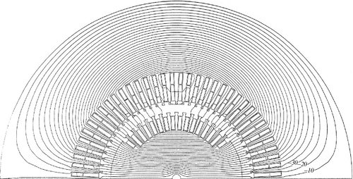
Numerical methods such as the finite-difference and finite-element methods [18] enable the engineer to compute no-load and full-load magnetic fields and those associated with short-circuit and starting conditions, as well as fields for the calculation of leakage, synchronous, transient, and subtransient inductances or reactances. Figures 4.2, 4.3, and 4.4 represent the no-load, short-circuit, and full-load fields, respectively, of a four-pole generator [19,20]. Figure 4.3 illustrates the winding forces during steady-state short-circuit conditions. These forces were computed based on the “Maxwell stress” discussed later in this chapter. Figure 4.2b [21] shows that at rated voltage only a small amount of flux (e.g., 1.4 mT) enters the space between the iron core (stator back iron) and the stator frame, and the eddy currents induced in the solid key bars are negligible. Figures 4.5 and 4.6 illustrate synchronous linear Ld, Lq inductances or synchronous Xd, Xq reactances [19,20,22] of a two-pole generator. Figures 4.5 and 4.6 do not indicate any coupling between the d- and q-axes. Such a coupling is due to the saturation and is called cross-coupling [23], which will be neglected in subsequent sections. Figure 4.7 pertains to the calculation of the transient inductance Ld′ or transient reactance Xd′ [19,22]. Figure 4.8 illustrates the field of a two-pole generator at full load.


In general, for synchronous machines with a field-current excitation in the d-axis the following inequalities are valid: Xd ≥ Xq, Xd′ ≤ Xq′, and Xd″ ≤ Xq″. However, for inverter-fed synchronous machines with permanent-magnet excitation – also called brushless DC machines – as used in high-efficiency, variable-speed drives [24,25], due to the lack of field and damper windings in such machines, the transient and subtransient reactances are not defined. Figures 4.9 and 4.10 depict no-load and full-load fields of a permanent-magnet machine, respectively, whereas Fig. 4.11 illustrates the field for the calculation of the stator self-inductance (e.g., Lq). In permanent-magnet machines the leakage is defined as the leakage flux between two stator winding phases and not the leakage flux between the stator and the rotor windings (which do not exist) as it is normally defined for other types of machines. In addition Lq is larger than Ld, and there is a significant amount of cogging [26].


4.2.1 Definition of Transient and Subtransient Reactances as a Function of Leakage and Mutual Reactances
The dq0 model requires the availability of values for the synchronous (Xd, Xq), transient (Xd′, Xq′), and subtransient (Xd″, Xq″) reactances of synchronous machines. Most turbogenerators have field windings in the d-axis only and none in the q-axis, therefore ![]() . The transient reactance Xd′ can be defined in terms of leakage and mutual reactances, as depicted in Fig. 4.12:
. The transient reactance Xd′ can be defined in terms of leakage and mutual reactances, as depicted in Fig. 4.12:

where Xal is the amature (stator) leakage reactance, Xfl is the field leakage reactance, and Xaf is the mutual reactance between armature and field circuits.

Correspondingly, one obtains for the subtransient reactance Xd″ (Fig. 4.13):

where Xdl is the d-axis damper winding leakage reactance.

Representative per-unit values for a typical turbogenerator are
In general, 1 pu ≤ Xd ≤ 2 pu, 1 pu ≤ Xq ≤ 2 pu, 0.2 pu ≤ Xd′ ≤ 0.4 pu, 0.1 pu ≤ Xd″ ≤ 0.3 pu, and the values of Xq′ and Xq″ depend on the field and damper winding design within the q-axis, respectively. Note that the value of Xq″ depends on the rotor construction and the damper winding associated with the q-axis: if there are no additional damper bars located on the rotor pole, then Xq″ is relatively large and in the neighborhood of Xq. In the presence of damper windings in the q-axis Xq″ is somewhat larger than Xd″ because the damper winding (e.g., solid rotor or embedded damper bars on the rotor pole) of the q-axis is less effective than that of the d-axis. The rationale for selecting the above ranges for the various reactances lies in the stability requirements for generators when operating on the power system: machines with small reactances exhibit better stability than machines with large reactances; or in other words, machines with small reactances or inductances have smaller time constants than those with large reactances or inductances. Small reactances require a large air gap and a large field current for setting up the maximum flux density across the air gap of about Bmax = 0.7 T. The large air gap makes machines less efficient as compared to those with small air gaps. One has to weigh the benefits of a more stable but less efficient machine versus that with less stability but greater efficiency. In addition, machines with small reactances result in larger short-circuit currents and larger transient torques and winding forces than machines with larger reactances.
4.2.2 Phasor Diagrams for Round-Rotor Synchronous Machines
There are two ways of drawing equivalent circuits and phasor diagrams of synchronous machines. The first one is based on the so-called consumer system, where the terminal current flows into the equivalent circuit, and the second one is the generator system, where the terminal current flows out of the equivalent circuit. The first one is mostly employed by engineers concerned with drives, and the latter one is mostly used by power system engineers who are concerned with generation issues.
4.2.2.1 Consumer (Motor) Reference Frame
Figure 4.14a depicts the equivalent circuit of a round-rotor synchronous machine based on the consumer (motor) reference current system. Figure 4.14b illustrates the corresponding phasor diagram for overexcited operation, and Fig.4.14c pertains to underexcited operation. Note that the polarity of the voltages is indicated by + and – signs as well as by arrows, where the head of the arrow coincides with the + sign and the tail of the arrow with the – sign. Such an arrow notation makes it easier to draw phasor diagrams. The phasor diagrams are not to scale because the ohmic voltage drop ![]() R is normally much smaller than the reactive voltage drop
R is normally much smaller than the reactive voltage drop ![]() X.
X.

4.2.2.2 Generator Reference Frame
Figure 4.15a depicts the equivalent circuit of a round-rotor synchronous machine based on the generator reference current system. Figure 4.15b,c illustrate the corresponding phasor diagram for overexcited and underexcited operation, respectively.

4.2.2.3 Similarities between Synchronous Machines and Pulse-Width-Modulated (PWM) Current-Controlled, Voltage-Source Inverters
Inverters are electronic devices transforming voltages and currents from a DC source to an equivalent AC source. Figure 4.16a illustrates the actual circuit of an inverter, where the input voltage is a DC voltage Vdc and the output voltage is an AC voltage ![]() . It is assumed that the PWM switching is lossless. In Fig. 4.16b the DC voltage (Vdc/2) is transformed to the AC side and represented by the phasor (
. It is assumed that the PWM switching is lossless. In Fig. 4.16b the DC voltage (Vdc/2) is transformed to the AC side and represented by the phasor (![]() /2), which makes the equivalent circuit of Fig. 4.16b similar to that of a round-rotor synchronous machine, as depicted in Fig. 4.15a. The relation between the (fundamental) output voltage |
/2), which makes the equivalent circuit of Fig. 4.16b similar to that of a round-rotor synchronous machine, as depicted in Fig. 4.15a. The relation between the (fundamental) output voltage |![]() | of the inverter and the input voltage
| of the inverter and the input voltage ![]() /2 (transformed to the AC side) is given [28] by
/2 (transformed to the AC side) is given [28] by

where m ≤ 1 is the modulation index of the (sinusoidal) PWM. This relation appears to hold for operation around unity displacement (fundamental power) factor only for m = 1 [29,30]. In these references it is shown that at lagging (overexcited, delivering reactive power to the grid) displacement power factor a higher input voltage Vdc than specified by Eq. 4-26 is required, whereas for leading (underexcited, absorbing reactive power from the grid) displacement power factor a smaller input voltage Vdc is sufficient. For example, although for unity displacement factor Vdc_unity_pf = 400 V is acceptable, a higher input voltage, e.g., Vdc_lagging_pf = 600 V is required for displacement factors larger than cos φ = 0.8 lagging (overexcited) [29,30] at |![]() | = 139 V, where m = 0.66.
| = 139 V, where m = 0.66.

 dc/2 is referred to the secondary side.
4.2.2.4 Phasor Diagram of a Salient-Pole Synchronous Machine
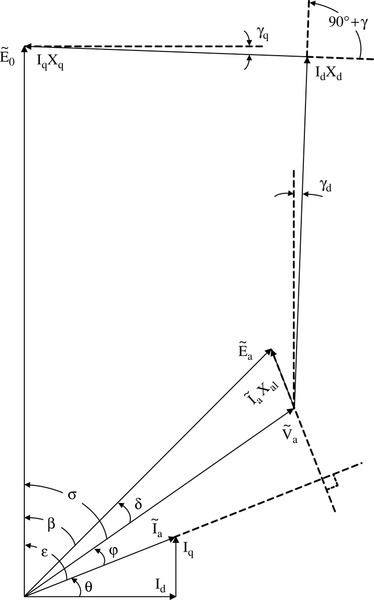
The d- and q-equivalent circuits and the associated phasor diagram of a (balanced) salient-pole synchronous machine are given in Fig. 4.17a,b,c. Note there is no zero-sequence equivalent circuit, which becomes important for unbalanced operation (e.g., asymmetrical short-circuits) of synchronous machines only. Figure 4.17c represents the phasor diagram without cross-coupling between the d- and q-axes due to saturation. The relation between voltages, currents, and reactances is given by the phasor diagram of Fig. 4.18 including cross-coupling of d- and q-axes parameters [20,23]. This cross-coupling is due to saturation of the machine and will be neglected in subsequent sections.

According to [7] the following relations are valid.
Terminal voltage component in d-axis as a function of the fluxes and currents in d- and q-axes:
Terminal voltage component in q-axis:
Eqs. 4-27 and 4-28 solved for Id and Iq yield


which may be written in terms of the terminal voltage ![]() :
:


where
4.2.3 Application Example 4.1: Steady-State Analysis of a Nonsalient-Pole (Round-Rotor) Synchronous Machine
A three-phase (m = 3), four-pole (p = 4) nonsalientpole (round-rotor) synchronous machine has the parameters XS = 2 pu and Ra = 0.05 pu. It is operated at (the phase voltage) Va = 1 pu at an overexcited (lagging current based on the generator reference system, where the current flows out of the machine) displacement power factor of cos φ = 0.8 lagging, and per-phase current ![]() = 1 pu. The base (rated phase) values are
= 1 pu. The base (rated phase) values are ![]() = Vbase = 24 kV,
= Vbase = 24 kV, ![]() = Ibase = 1.4 kA, and the base impedance is Zbase = Vbase/Ibase = 17.14 Ω.
= Ibase = 1.4 kA, and the base impedance is Zbase = Vbase/Ibase = 17.14 Ω.
a) Draw the per-phase equivalent circuit of this machine.
b) What is the total rated apparent input power S (expressed in MVA)?
c) What is the total rated real input power P (expressed in MW)?
d) Draw a per-phase phasor diagram with the voltage scale of 1.0 pu ≡ 3 inches, and the current scale of 1.0 pu ≡ 2.5 inches.
e) From this phasor diagram determine the per-phase induced voltage |Ẽa| and the torque angle δ.
f) Calculate the rated speed (in rpm) of this machine at f = 60 Hz.
g) Calculate the angular velocity ωS (in rad/s).
h) Calculate the total (approximate) shaft power Pshaft ≈ 3(Ea · Va · sin δ)/XS.
i) Find the shaft torque Tshaft (in Nm).
j) Determine the total ohmic loss of the motor ![]() .
.
k) Repeat the above analysis for cos φ = 0.8 underexcited (leading current based on generator notation) displacement power factor and ![]() = 0.5 pu.
= 0.5 pu.
Solution to Application Example 4.1
a) The per-phase equivalent circuit of a nonsalient-pole synchronous machine based on generator notation is shown in Fig. 4.15a. The parameters of the machine are in ohms: ![]()
b) ![]() (E4.1-1)
(E4.1-1)
c) ![]() (E4.1-2)
(E4.1-2)
d) The phasor diagram is given in Fig. E4.1.1.

![]() = 1 pu = 24 kV ≡ 3 inches,
= 1 pu = 24 kV ≡ 3 inches,![]() = 1 pu = 1.4 kA ≡ 2.5 inches,
= 1 pu = 1.4 kA ≡ 2.5 inches,![]() · Ra = 1.4kA(0.05)(17.141 Ω) = 1199.8 V ≡ 0.15 inches,
· Ra = 1.4kA(0.05)(17.141 Ω) = 1199.8 V ≡ 0.15 inches,![]() · Xs = 1.4 kA(2)(17.141 Ω) = 47992 V ≡ 6 inches.
· Xs = 1.4 kA(2)(17.141 Ω) = 47992 V ≡ 6 inches.
e) For the induced voltage one obtains

where![]() = 0.05 pu, sin φ = 0.6, and cos φ = 0.8.
= 0.05 pu, sin φ = 0.6, and cos φ = 0.8.
The torque angle δ is
f) Rated speed is
g) Angular velocity is
h) Approximate shaft power is
i) The shaft torque Tshaft is
j) The total ohmic loss of the motor is
k) Repeat the above analysis for underexcited (leading current based on generator reference system) displacement power factor cos φ = 0.8 leading and ![]() = 0.5 pu.
= 0.5 pu.
a) see Fig. 4.15a
b) Srated = 3 · Va_rated · Ia_rated = 3(24 kV)(0.7kA) = 50.4 MVA.
c) Prated = Srated · cos φ = 40.32 MW.
d) The phasor diagram is given in Fig. E4.1.2.


e) For the induced voltage one obtains

where![]() = 1 pu,
= 1 pu, ![]() = 1 pu,
= 1 pu, ![]() = 0.025 pu, sin φ = 0.6, cos φ = 0.8.
= 0.025 pu, sin φ = 0.6, cos φ = 0.8.
The torque angle δ is
f) Rated speed is
g) Angular velocity is ωS = 2πnS/60 = 188.7 rad/s.
h) Approximate shaft power is
i) The shaft torque Tshaft is Tshaft = Pshaft/ωS = 217.75 kNm.
j) The total ohmic loss of the motor is
4.2.4 Application Example 4.2: Calculation of the Synchronous Reactance XS of a Cylindrical-Rotor (Round-Rotor, Nonsalient-Pole) Synchronous Machine
A p = 2 pole, f = 60 Hz synchronous machine (generator, alternator, motor) is rated Srat = 16 MVA at a lagging (generating reference system) displacement power factor cos φ = 0.8, a line-to-line terminal voltage of VL-L = 13,800 V, and a (one-sided) air-gap length of g = 0.0127 m. The stator has 48 slots and has a three-phase double-layer, 60° phase-belt winding with 48 armature coils having a short pitch of 2/3. Each coil consists of one turn Ncoil = 1. Sixteen stator coils are connected in series, that is, the number of series turns per phase of the stator (st) are Nst phase = 16 (see Fig. E4.2.1). The maximum air-gap flux density at no load (stator current Ist phase = 0) is Bst max = 1 T.

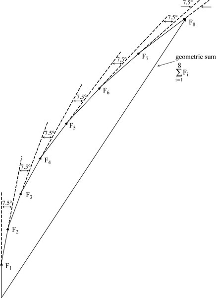
There are eight field coils per pole (see Fig. E4.2.2) and they are pitched 44-60-76-92-124-140-156-172 degrees, respectively, as indicated in Fig. E4.2.2. Each field coil has 18 turns. The developed rotor (field) magnetomotive force (mmf) Fr is depicted in Fig. E4.2.3. Note that the field mmf is approximately sinusoidal.


a) Calculate the distribution (breadth) factor of the stator winding kstb (= kstd).
b) Calculate the fundamental pitch factor of the stator winding kstp1.
c) Calculate the pitch factor of the rotor (r) winding krp.
d) Determine the stator flux Φstmax.
e) Compute the area (areap) of one pole.
f) Compute the field (f) current Ifo required at no load.
g) Determine the synchronous (s) reactance (per phase value) XS of this synchronous machine in ohms.
h) Find the base impedance Zbase expressed in ohms.
i) Express the synchronous reactance XS in per unit (pu).
Solution to Application Example 4.2
a) Calculation of the distribution (breadth) factor of the stator winding kstb = kstd is as follows. The breadth factor is defined for one phase belt as

It is convenient to evaluate Eq. E4.2-1 graphically, as shown in Fig. E4.2.4. Note that one slot pitch corresponds to 360°/48 = 7.5°. Thus, one gets from Fig. E4.2.4 the distribution or breadth factor
b) Calculation of the pitch factor of the stator winding kstp1 is as follows. One stator turn spans 16 slots out of 24 slots, that is, it has a pitch of (2/3); therefore, one obtains for the fundamental n = 1

or for the 5th harmonic n = 5

The 5th harmonic is not attenuated; therefore, the choice of a 2/3 winding pitch is not recommended.
The total fundamental winding factor of the stator winding is now
c) Calculate the pitch factor of the rotor (r) winding krp as follows. The fundamental (n = 1) pitch-factor of the rotor winding is correspondingly


d) Determination of the stator flux Φstmax is as follows. The induced voltage in the stator winding per phase is
or one obtains for the stator flux

with EL-L = VL-L = 13,800 V at no load, one gets the flux for no-load condition:

e) Compute the area (areap) of one pole:

f) Compute the field (f) current Ifo required at no load:

g) Determine the synchronous (s) reactance (per phase value) XS in ohms. The self-inductance of phase a is


According to Concordia [7]
Neglecting Laa2 and Laa ≈ Lab one gets for the synchronous inductance Ld
The synchronous reactance of the round-rotor machine is
The base voltage is

The base apparent power is per phase
and the base current is

h) Find the base impedance Zbase expressed in ohms. The base impedance becomes

i) Express the synchronous reactance XS in per unit (pu). The per-unit synchronous reactance is now

4.2.5 Application Example 4.3: dq0 Modeling of a Salient-Pole Synchronous Machine
Engineers are most concerned about the torques generated by the machine under abnormal operating conditions such as:
• balanced three-phase short-circuit,
• line-to-line short-circuit,
• line-to-neutral short-circuit,
• out-of-phase synchronization,
• synchronizing and damping torques,
• reclosing, and
• stability.
Linear (not saturation-dependent) reactances are assumed and amortisseur (damper) windings are neglected except for some out-of-phase synchronization results and for reclosing events. Most machines have very weak damper windings and, therefore, this assumption is justified. Synchronizing TS and damping TD torques of the salient-pole synchronous machine using dq0 modeling are also addressed in Problem 4.8.
Solution to Application Example 4.3
a) Balanced Three-Phase Short-Circuit. If the terminals of a synchronous generator are short circuited at rated no-load excitation one obtains the balanced short-circuit currents in per unit [31]:


where tan δ = ![]() , φ = ωt.
, φ = ωt.
The field current is

and the torque is

The maximum torque occurs at the angle φmax which can be obtained from

Figure E4.3.1 illustrates the torque of Eqs. E4.3-5 and E4.3-6.

b) Line-to-Line Short-Circuit. The short-circuit of the two terminals b and c of a synchronous generator results in the line-to-line short-circuit current [31]

or for φo = 0

and the torque is

or

Figure E4.3.2 illustrates the torques of Eqs. E4.3-5, E4.3-6, and E4.3-10.

The open-circuit voltage induced in phase a in case of a short-circuit of line b with line c is

where
The maximum value of ea occurs for φo = 0
Figure E4.3.3 illustrates the induced voltage ea of Eqs. E4.3-11 and E4.3-12a,b.

c) Line-to-Neutral Short-Circuit. The current when phase a of a synchronous machine at no load is short-circuited is for θ = 90° + φ [31]

or in terms of an infinite series

where

Note that ia must be initially zero, that is, φ = φo = 0 or θo = 90°.
The fundamental component becomes now

or in terms of symmetrical components

d) Out-of-Phase Synchronization. When synchronizing a generator (either machine or inverter) with the power system the following conditions must be met:
• phase sequence must be the same,
• the phase angle between the two voltage systems must be sufficiently small, and
• the slip must be small.
Synchronizing out of phase is an important issue because it generates the highest torques and forces (in particular within the end winding of a machine) when paralleled with the power system [31]. The torque during out-of-phase synchronization is as a function of time φ = ωt and the angle δ between the power system’s voltage and that of the synchronous machine voltage at the time of paralleling:

Note this expression is symmetrical in δ and φ, that is, δ and φ can be interchanged without altering the relation. Introducing δ = φ in Eq. E4.3-18, one obtains for the torque

The corresponding field current is

Figure E4.3.4 illustrates the very large torque if the generator is out-of-phase synchronized with the worst case angle of δ = 141.5° and when φ = δ in Eq. E4.3-18.

Experimental results [32–34] during out-of-phase synchronization show that for small synchronous machines below 100 kVA a voltage difference of ΔV ≤ ± 10%, a phase angle difference of Δδ ≤ ± 5°, and a slip of s ≤ 1% can be permitted. For large machines these conditions must be more stringent; that is, the voltage difference ΔV ≤ ± 1%, the phase angle difference Δδ ≤ ± 0.5°, and the slip s ≤ 0.1%. During the past first analog [32–34] and then digital paralleling devices have been employed to connect synchronous generators to the grid. Although these devices are very reliable, once in a while a faulty paralleling occurs.
Figure E4.3.5 depicts the various parameters when out-of-phase synchronization occurs with an angle of δ = 255° – which is not the worst-case condition (see Fig. E4.3.4). In this analysis subtransient reactances are taken into account.

• Stator currents ia, ib, and ic are amplitude modulated and reach maximum values of 4 pu;
• Zero-sequence component current (io = ia + ib + ic) flowing in the grounded neutral is relatively small and about 0.5 pu;
• Electrical generator (G) torque TG assumes a maximum value of about 4 pu;
• Rotor (torque) angle exceeds 90°;
• Real PG and reactive QG power oscillations occur;
• Slip s reaches values of more than 3 pu; and
• Mechanical torque TM between generator and turbine is below 1 pu.
Not shown in this graph are the extremely large winding forces in the end region of the stator winding, and the excessive heating of the amortisseur bars and the solid-rotor pole face. The latter issue will be addressed in a later example. In Fig. E4.3.5 the left scale pertains to the dotted signals and the right scale belongs to the full-line signals.
Figure E4.3.6a illustrates the conditions under which a 30 kVA inverter of a wind-power plant was paralleled with the power system [29,30]. The switching frequency and therefore the fundamental (nominally 60 Hz) frequency was phase-locked with the power system’s frequency and thus the slip is by definition s = 0. However, the voltage differences and the phase differences must be within certain limits. Experiments showed it was advisable to choose the inverter rms value of the line-to-line voltage always somewhat larger (e.g., VL-Linverter = 260 Vrms) than that of the power system’s line-to-line voltage (e.g., VL-Lpower system = 240 Vrms). Figure E4.3.6b depicts the transient current flowing from inverter to power system when inverter is paralleled at an inverter voltage of VL-Linverter = 260 Vrms at an out-of-phase voltage angel of δ = 24°, where the inverter voltage leads that of the power system. As can be seen, the transient current is more than 200 A.
Figure E4.3.7 illustrates the stator flux distribution when a large synchronous generator is paralleled out-of-phase [21]: the stator flux leaves the iron core (stator back iron) and currents are induced in the key bars of the iron-core suspension as well as in the aluminum bars within the dovetails of the iron core. The flux density within the space between the iron core and the frame is 17 mT at a terminal voltage of 1.23 pu. This flux density is sufficient to heat up the solid iron key bars and melt the aluminum bars within the dovetails of the iron core.


e) Synchronizing and Damping Torques. When a synchronous generator is paralleled with the power system one obtains for the angle perturbation Δsin ωt from the steady-state angle δ0 the synchronizing TS and damping TD torques in addition to the steady-state torque T0 [31]:
where

where Vℓ-no is the open-circuit phase (line-to-neutral) voltage at steady-state operation, Vℓ-n is the phase (line-to-neutral) voltage during synchronization and is approximately ![]()

where Vℓ-no is the open-circuit phase (line-to-neutral) voltage at steady-state operation, Vℓ-n is the phase (line-to-neutral) voltage during synchronization and is approximately Vℓ-no ≈ Vℓ-n ( ≈ 1.0 pu).

where

f) Torques during Reclosing. In order to minimize power quality problems after short-circuits have occurred, it is common practice to reclose the switches that have been opened due to the short-circuit. Short-circuits can be interrupted within four to six 60 Hz cycles. In the hope that the short-circuit has been cleared, the utilities reclose the previously opened switches after nine to fifteen 60 Hz cycles have elapsed. If the short-circuit still persists, then the fault will be cleared again after additional four to six 60 Hz cycles. At the most three to five reclosing operations are performed. The timing of the reclosing is important: if the timing is unfavorable the mechanical torques of the turbine stages become excessive, but under favorable conditions these mechanical torques can be minimized. Only an accurate dynamic calculation can approximately predetermine the most favorable reclosing times. Transient electromagnetic and shaft torques of synchronous generators can become as high as 5–6 during reclosing [35–39]. The magnitudes of the torques depend on the reclosing time. If the reclosing occurs at a time when the electrical torque due to reclosing adds to the transient shaft torque, the resulting mechanical shaft becomes large as compared to the case where the electrical torque due to the reclosing opposes the transient shaft torque; in the latter case the resulting shaft torque will be relatively small. This amplification effect of the mechanical transient torque has its analogy in the “swing effect” one encounters on a playground.
Joyce et al. [35,36] have recommended introducing a measure for the theoretical lifetime of a turbine shaft: the occurrence of many high torsional torques reduces the lifetime of a shaft more quickly than the occurrence of low torsional torques. Figure E4.3.8 illustrates a common connection of a power plant to the high-voltage system. One generator feeds two transformers, which are connected to high-voltage feeders each. This is to minimize the outage of a power plant due to external faults such as short-circuits within the power system. The short-circuit is caused by making the impedances ZFa, ZFb, and ZFc zero. Breaker #2 interrupts the short-circuit and recloses after a preprogrammed time.
Figures E4.3.9a and E4.3.9b depict the various parameters when reclosing with different reclosing times but with the same short-circuit duration (104 ms) occurs. In these graphs the left scale pertains to the dotted signals and the right scale belongs to the full-line signals.
Summarizing one can state the following:


• During the three-phase short-circuit the stator currents ia, ib, and ic are amplitude modulated and exceed maximum values of 4 pu;
• Zero-sequence component current (io = ia + ib + ic) flowing in the grounded neutral is relatively large and exceeds 4 pu;
• Electrical torque TG assumes a maximum value of about 3 pu;
• Rotor (torque) angle is below 90°;
• Very large (about 2 pu) real PG and reactive QG power swings occur;
• Maximum slip reaches values of more than 1 pu;
• Mechanical torque TM between generator and turbine is below 1 pu, but it has an alternating component causing mechanical stress; and
• In both cases the stability of the synchronous generators is maintained due to the torque angle δ being less than 90°.
Not shown in the graphs are the extremely large winding forces in the end region of the stator winding, and the excessive heating of the amortisseur bars residing on the rotor. As can be expected, the electrical and mechanical stresses depend on the reclosing times, which are 450 ms and 745 ms for Figs. E4.3.9a and E4.3.9b, respectively.
4.2.6 Application Example 4.4: Calculation of the Amortisseur (Damper Winding) Bar Losses of a Synchronous Machine during Balanced Three-Phase Short-Circuit, Line-to-Line Short-Circuit, Out-of-Phase Synchronization, and Unbalanced Load Based on the Natural abc Reference System [40]
For the analysis of subtransient phenomena, a simulation of the damper-winding system of alternators is of utmost importance. Concordia [7] expanded the usual d- and q-axes decomposition by introducing more than two (e.g., d and q) damper winding systems. In this application example the amortisseur is approximated by 16 damper windings in the d- and q-axes as shown in Fig. E4.4.1, that is, 8 damper windings in the d-axis and 8 damper windings in the q-axis. Damper bars reside in the rotor slots and some bars are embedded in the solid rotor pole zone. To simplify this analysis it is assumed that the rotor is laminated; that means no eddy currents are induced, saturation is neglected, and there are no damper bars embedded in the pole zone.
