
Solution to Application Example 4.4
Following the notation of [7] one obtains the voltage equations:
ea=pΨa−r⋅ia
eb=pΨb−r⋅ib
ec=pΨc−r⋅ic
efd=pΨfd+rfd⋅ifd
0=pΨkd−rkd⋅ikd+vkd
0=pΨkq−rkq⋅ikq+vkq
for k = 1, 2, 3, …, 8 damper windings in d- or q-axes.
The flux linkage equations are
Ψa=−Laaia−Labib−Lacic+Lafdifd+Lakdikd+Lakqikq
Ψb=−Lbaia−Lbbib−Lbcic+Lbfdifd+Lbkdikd+Lbkqikq
Ψc=−Lcaia−Lcbib−Lccic+Lcfdifd+Lckdikd+Lckqikq
Ψfd=−Lfdaia−Lfdbib−Lfdcic+Lfdfdifd+Lfdkdikd
Ψkd=−Lkdaia−Lkdbib−Lkdcic+Lkdfdifd+Lkd1di1d+Lkd2di2d+…+Lkdldild
Ψkq=−Lkqaia−Lkqbib−Lkqcic+Lkk1qi1q+Lkq2qi2q+…+Lkqlqilq
for k = 1, 2, …, 8 and l = 1, 2, …, 8.
Following the notation of Fig. E4.4.2, the self-inductance of the kth damper winding is
LRkd=2⋅ℓR⋅ARkd/Ikd
and the leakage inductance with respect to stator winding is
LRkdl=2⋅ℓR⋅(ARkd−ASkd)/Ikd
or referred to the stator reference frame, where m1 and m2 are the number of stator and rotor phases, respectively:
Lkd=m1(2⋅ℓR⋅ARkd/Ikd)M2kda/m2
Lkdl=m1{2⋅ℓR⋅(ARkd−ASkd)/Ikd}M2kda/m2.

The mutual inductances between the kth and the lth d-axis windings are
Lkdld=m1⋅Lkdkdld⋅M2kdld⋅M2lda/m2
Lldkd=m1⋅Lldldkd⋅M2ldkd⋅M2kda/m2.
Correspondingly the ohmic resistance is
rkd=m1⋅Rkd⋅M2kda/m2.
The same procedure applies to the q-axis parameters, as indicated in Fig. E4.4.3. In these equations ℓR is the rotor length. Mkda, Mkdld, Mlda, and Mldkd are transformation ratios. The calculation of the stator inductances (Fig. E4.4.4) is performed in the same manner as for the rotor inductances.


If Eqs. E4.4-2 to E4.4-8 are introduced in Eq. E4.4-1 one obtains
[L]⋅[didt]=[V],

where [L] is an inductance matrix with time-varying coefficients, [didt]![]() is the derivative of the solution vector [i] and [V] represents the forcing sources. Using Gaussian elimination one gets
is the derivative of the solution vector [i] and [V] represents the forcing sources. Using Gaussian elimination one gets
[didt]=[L]−1⋅[V].

Subsequently a Runge-Kutta integration procedure of the fourth order provides the first starting steps for the Adams-Moulton method, which is a predictor-corrector integration procedure, and one obtains the solution vector [i]. A line-to-line short-circuit including the generator-transformer leakage impedance is performed. The line-to-neutral voltages in per unit (referred to the rated voltage of the generator) are shown in Fig. E4.4.5. The stator currents are depicted in Fig. E4.4.6, and field and damper bar currents are shown in Figs. E4.4.7 and E4.4.8a,b. The resulting electrical and mechanical torques are depicted in Figs. E4.4.9 and E4.4.10.


The integral ∫t21(ikbar)2dt![]() is a measure for the energy absorbed by the damper bar k due to the current ikbar. Therefore, the energy dissipated in the damper bar k during time (t2 – t1) is
is a measure for the energy absorbed by the damper bar k due to the current ikbar. Therefore, the energy dissipated in the damper bar k during time (t2 – t1) is
Ekbar={∫t21(ikbar)2dt}Rkbar.

It is well known that the bar (e.g., #16) of the amortisseur (see Fig. E4.4.11) located before the rotor pole as viewed in the direction of rotation incurs greater loss than the bar (e.g., #1) of the amortisseur located behind the rotor pole as viewed in the direction of rotation. Figure E4.4.4.12 shows the values Ekbar for a sudden line-to-line short-circuit at the terminals including transformer impedance for various time intervals (t2 – t1). Figure E4.4.13 depicts the subtransient field of a generator during the first cycle of a three phase short-circuit.
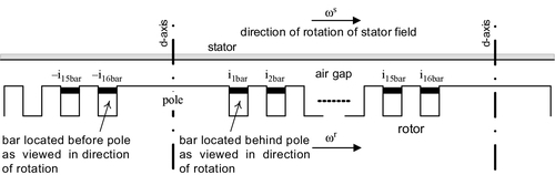


Table E4.4.1 summarizes the dissipated energies in the 1st and 16th amortisseur bars during various fault conditions of a generator including the generator-transformer leakage impedance:
Table E4.4.1
Dissipated Energies in Amortisseur Bars #1 and #16 for Different Fault Conditions
| Fault condition | Energy dissipated in per unita in bar #1 during first 1.25 s | Energy dissipated in per unita in bar #16 during first 1.25 s |
| Line-to-line short-circuit | 0.95 | 1.05 |
| Balanced three-phase short-circuit | 0.92 | 1.12 |
| Out-of-phase synchronization with a 120° leading rotor angle | 2.36 | 2.43 |
| Out-of-phase synchronization with a 120° lagging rotor angle | 1.25 | 1.57 |
| Unbalanced stator currents resulting in an inverse stator current of |˜I2 | 0.049 | 0.053 |
a Energy dissipated in a bar is referred to the heat energy required to melt one bar if there is no cooling.
1) line-to-line short-circuit,
2) balanced three-phase short-circuit,
3) out-of-phase synchronization with a 120° leading rotor angle,
4) out-of-phase synchronization with a 120° lagging rotor angle, and
5) unbalanced stator currents resulting in an inverse stator current of |˜I2![]() | | = 8.7%.
| | = 8.7%.
Discussion of Results
• Most transients decay within 1 to 2 s.
• The 2nd harmonic in the stator currents of Fig. E4.4.6 is confirmed by measurements.
• The thermal stress of the amortisseur bars due to a balanced short-circuit can be tolerated, provided there are no subsequent short-circuits within a brief time frame.
• An imbalance due to an inverse current of |˜I2![]() | = 8.7% is acceptable—even during steady-state operation.
| = 8.7% is acceptable—even during steady-state operation.
• There is a great difference when synchronizing with either a leading rotor angle or a lagging rotor angle. Out-of-phase synchronization with a leading rotor angle generates more losses within the generator than in the case of synchronization with a lagging rotor angle. In the first case the machine acts as a generator and in the latter it acts as a motor during the synchronization process. Note that an out-of-phase angle in the neighborhood of 140° leads to the largest currents and torques (see Fig. E4.3.4).
• To mitigate or reduce the thermal stress of damper bars #1 and #16 manufacturers of synchronous generators embed damper bars also on the surface of the rotor poles. In this manner the thermal stress of all amortisseur bars will be made more equal.
• Not neglecting saturation and the generation of eddy currents within the solid rotor poles will in addition mitigate the thermal stress of the entire amortisseur because the inductive coupling between stator and rotor damper windings will be reduced.
• A similar analysis applies to the induced currents of an induction machine. Under normal operation the currents induced in the rotor bars of an induction machine are uniform and have the same rated magnitude Ibar_rated in each and every bar. However, if a bar is broken (that is, no current can flow) then the neighboring bars will have currents that can be significantly larger than the rated magnitude. Such an unequal current distribution may result in a thermal imbalance. As a consequence due to this imbalance and the very small air gap of induction machines, the rotor may become eccentric and rub against the stator core, and this may lead to failure of the induction machine. See Chapter 3 for more details.
The abc-reference frame employed in this example has been subsequently used in references [41–43]. The above results are confirmed in these references. However, the out-of-phase synchronizing angle of 180° as used in [43] does not yield the largest currents, losses, and torques (see Fig. E4.3.4). These references teach that the large losses in the damper bars next to the poles (e.g., bar #1 and bar #16) can be reduced by the deployment of amortisseur bars, which are embedded within the pole faces.
4.2.7 Application Example 4.5: Measured Voltage Ripple of a 30 kVA Permanent-Magnet Synchronous Machine, Designed for a Direct-Drive Wind-Power Plant
A permanent-magnet generator is designed [29,30] for a variable-speed drive of a wind-power plant without any mechanical gear. The rated speed range is from 60 to 120 rpm. Line-to-neutral voltages vL-N and line-to-line voltages vL-L are recorded at no load and under rated load.
The voltage wave shapes are subjected to a Fourier analysis. Figures E4.5.1 and E4.5.2 depict the line-to-neutral voltages at no load and rated load, respectively, and Tables E4.5.1 and E4.5.2 represent their Fourier coefficients. Figures E4.5.3 and E4.5.4 represent the line-to-line voltages at no load and at rated load, and Tables E4.5.3 and E4.5.4 list their spectra. To minimize the size of this low-speed generator, the stator pitch kp and distribution kd winding factors are chosen relatively high (kp · kd = 0.8) resulting in a somewhat nonsinusoidal voltage wave shape. The generator feeds a rectifier and for this reason the nonsinusoidal voltage wave shape does not matter, except it increases the generator losses within acceptable limits.


Table E4.5.1
Harmonic Spectrum of Fig. E4.5.1
| Harmonic order | Harmonic magnitude (%) | Harmonic order | Harmonic magnitude (%) |
| 1 | 100 | 7 | 3 |
| 2 | 0 | 8 | 0 |
| 3 | 11 | 9 | 8 |
| 4 | 0 | 10 | 0 |
| 5 | 1 | 11 | 7 |
| 6 | 0 | 12 | 0 |

Table E4.5.2
Harmonic Spectrum of Fig. E4.5.2
| Harmonic order | Harmonic magnitude (%) | Harmonic order | Harmonic magnitude (%) |
| 1 | 100 | 7 | 2 |
| 2 | 0 | 8 | 0 |
| 3 | 14 | 9 | 7 |
| 4 | 0 | 10 | 0 |
| 5 | 1 | 11 | 5 |
| 6 | 0 | 12 | 0 |


Table E4.5.3
Harmonic Spectrum of Fig. E4.5.3
| Harmonic order | Harmonic magnitude (%) | Harmonic order | Harmonic magnitude (%) |
| 1 | 100 | 7 | 3 |
| 2 | 1 | 8 | 0 |
| 3 | 0 | 9 | 0 |
| 4 | 1 | 10 | 0 |
| 5 | 1 | 11 | 6 |
| 6 | 0 | 12 | 0 |

Table E4.5.4
Harmonic Spectrum of Fig. E4.5.4
| Harmonic order | Harmonic magnitude (%) | Harmonic order | Harmonic magnitude (%) |
| 1 | 100 | 7 | 3 |
| 2 | 1 | 8 | 0 |
| 3 | 1 | 9 | 0 |
| 4 | 0 | 10 | 0 |
| 5 | 1 | 11 | 6 |
| 6 | 0 | 12 | 0 |

4.2.8 Application Example 4.6: Calculation of Synchronous Reactances Xd and Xq from Measured Data Based on Phasor Diagram
Synchronous reactances are defined for fundamental frequency. Subjecting the voltage and current to a Fourier series yields the following data: line-to-neutral terminal voltage V(l-n), phase current I(l-n), instead of the induced voltage E the no-load voltage V(l-n)_no-load ≈ E can be used for a permanent-magnet machine if saturation is not dominant. The displacement power factor angle φ and the torque angle δ can be determined from an oscilloscope recording and from a stroboscope, respectively. The ohmic resistance R can be measured as a function of the machine temperature. The relationship between these quantities is given by the phasor diagram of Fig. E4.6.1. Calculate the synchronous reactances Xq and Xd.

Solution to Application Example 4.6
From the phasor diagram of Fig. E4.6.1, the following relations for the synchronous reactances Xq and Xd are derived:
Xq=V(l−n)sinδ+RI(l−n)sinδcosφ+RI(l−n)cosδsinφI(l−n)cosφcosδ−I(l−n)sinφsinδ,

Xd=E−V(l−n)cosδ+RI(l−n)cos(δ+φ)I(l−n)cos(90°−φ−δ).

An application of these relations is given in [44].
4.2.9 Application Example 4.7: Design of a Low-Speed 20 kW Permanent-Magnet Generator for a Wind-Power Plant
A P = 20 kW, VL-L = 337 V permanent-magnet generator has the cross sections of Figs. E4.7.1 and E4.7.2. The number of poles is p = 12 and its rated speed is nrat = nS = 60 rpm, where nS is the synchronous speed. The B–H characteristic of the neodymium–iron–boron (NdFeB) permanent-magnet material is shown in Fig. E4.7.3.


a) Calculate the frequency f of the stator voltages and currents.
b) Apply Ampere’s law to path C (shown in Figs. E4.7.1 and E4.7.2) assuming the stator and rotor iron cores are ideal (μr → ∞).
c) Apply the continuity of flux condition for the areas Am and Ag (representing half of the magnet area per pole and half of the air-gap area per pole, respectively) perpendicular to path C (two times the one-sided magnet (m) length lm, and two times the one-sided air gap (g) length lg, respectively). Furthermore lm = 7 mm, lg = 1 mm, Am = 11,668 mm2, and Ag = 14,469 mm2.
d) Provided the relative permeability of the stator and rotor cores is μr → ∞, compute the load line of this machine. Plot the load line in a figure similar to that of Fig. E4.7.3. Is the permanent-magnet material (NdFeB) operated at the point of the maximum energy product?
e) What is the recoil permeability μR of the NdFeB material?
f) Compute the fluxes Φmax and Φtotalmax = 2Φmax, provided there are N = 360 turns per stator phase, the (pitch and distribution) winding factor is kw = 0.8, and the iron-core stacking factor is kfe = 0.94.
g) Determine the diameter D of stator wire for a copper-fill factor of kcu = 0.62 and a stator slot cross section of Ast_slot = 368 mm2.
Solution to Application Example 4.7
ns=120fporf=nsp120=60(12)120=6Hz.

b) Ampere’s law
Hmlm+Hglg=0.
c) Continuity of flux
Φ=BmAm=BgAg,
d) Constituent relation
Bg=μ0Hg.
From Eq. E4.7-2
Hmlm=−Hglg.
With Eq. E4.7-4
Hmlm=−Bglg/μ0,
and with Eq. E4.7-3
Bg=Bm(AmAg),

the load-line equation becomes
Hm=−(AmAg)(lglm)Bmµ0.

Introducing the given numerical values into load-line equation gives
Hm=−91.7Bm[kAm].

This equation is plotted in Fig. E4.7.4. Note that the magnet material is not operated in the point of the maximum energy product.

e) Recoil permeability of NdFeB (slope of the permanent-magnet characteristic)
μR=(y2−y1)(x2−x1)=(Br−0)(0−(−Hc))=1.25950(103)=1.316×10⁻⁶(H/m)

or
μR=1.047μ0.
f) Induced voltage
Φmax=BmAm,
Φtotalmax=2Φmax=2BmAm,
The flux is defined as
Φ(t)=Φtotalmaxcosωt.
Therefore, the induced voltage is
Emax=N(dΦ/dt)=ωNphkwkfeΦtotalmax.
From load line and magnet characteristic one obtains the operating point:
Bm0=1.1T,
Hm0=−100kA/m.
Therefore,
Φ=Φtotalmax=(2)(1.1)(11668×10−6)Wb=0.0257Wb
and the induced voltage is now
e(t)=(360)(0.0257)(2π)(6)(0.8)(0.94)sinωt=Emaxsinωt,
or
Emax=262.3V,
Erms=Emax/√2=185.48V,
and the line-to-line terminal voltage is approximately
VL−L=√3VL−N=√3(1.05)Erms=337.3V,
g) Determination of wire diameter of the stator winding. Figure E4.7.5 depicts the stator winding housed in 72 slots. It is a full-pitch, double-layer winding. Using a copper-fill factor of kcu = 0.62 one obtains for a stator slot cross section of Ast_slot = 368 mm2 and (360/12) = 30 turns per stator pole and per phase with the copper cross section of one stator slot Ast_slot_cu = Ast_slot · kcu = 368 · 0.62 mm2 = 30πD2/4 or a wire diameter of D = 3.1 mm. For a rated current of Irat = 31 A one obtains a current density of J = 31/7.6 = 4.07 A/mm2. This current density is acceptable for a ventilated machine.

4.2.10 Application Example 4.8: Design of a 10 kW Wind-Power Plant Based on a Synchronous Machine
Design a wind-power plant (Fig. E4.8.1) feeding Pout_transformer = 10 kW into the distribution system at a line-to-line voltage of VL-L system = 12.47 kV = VL-L_secondary of transformer. The wind-power plant consists of a Y–Δ three-phase (ideal) transformer connected between three-phase PWM inverter and power system, where the Y is the primary and Δ is the secondary of the ideal transformer (Fig. E4.8.2). The input voltage of the PWM inverter (see Chapter 1, Fig. E1.5.1) is VDC = 600 V, where the inverter delivers an output AC current Iinverter at about 18° lagging displacement power factor (consumer notation) cos φ ≈ 0.95 lagging the primary line-neutral voltage of the Y – Δ transformer, and the inverter output line-to-line voltage is VL-L_inverter = 240 V = VL-L_primary of transformer.


The three-phase rectifier (see Chapter 1, Fig. E1.2.1) with one self-commuted PWM-operated switch (IGBT) is fed by a three-phase synchronous generator. The input line-to-line voltages of the three-phase rectifier is VL-L rectifier = 480 V = VL-L_generator. Design the mechanical gear between wind turbine and generator (with p = 2 poles at nS = 3600 rpm, utilization factor C = 1.3 kWmin/m3, Drotor = 0.2 m, the leakage reactance Xsleakage = 2πfLsleakage is 10% of the synchronous reactance XS = 1.5 pu, maximum flux density Bmax = 0.7 T, iron-stacking factor kfe = 0.95, stator winding factor kS = 0.8, rotor winding factor kr = 0.8, and torque angle δ = 30°) so that a wind turbine can operate at nturbine = 30 rpm. Lastly, the wind turbine – using the famous Lanchester-Betz-Joukowsky limit [45,84–86] for the maximum energy efficiency of a wind turbine as a guideline – is to be designed for the rated wind velocity of v = 10 m/s at an altitude of 1600 m and a coefficient of performance (actual efficiency) cp = 0.3. You may assume that all components (transformer, inverter, rectifier, generator, mechanical gear) except the wind turbine have each an efficiency of η = 95%.
a) Based on the given transformer output power of Pout_transformer = 10 kW compute the output powers of inverter, rectifier, generator, gear, and wind turbine.
b) For the circuit of Fig. E4.8.1 determine the transformation ratio (NY/NΔ) of the Y–Δ transformer, where the Y is the primary (inverter side) and Δ the secondary (power system side).
c) What is the phase shift between ˜V![]() L- L system and ˜V
L- L system and ˜V![]() L - L_inverter?
L - L_inverter?
d) What is the phase shift between ˜IL−system![]() and ˜IL−inverter
and ˜IL−inverter![]() ?
?
e) Use sinusoidal PWM to determine for the circuit of Fig. E1.5.1 the inverter output current Ĩinverter which lags ˜V![]() L - N_inverter = 138.57 V about 18° at an inverter switching frequency of fsw = 7.2 kHz. You may assume Rsystem = 50 mΩ, Xsystem = 0.1 Ω, Rinverter = 10 mΩ, and Xinverter = 0.377 Ω at f = 60 Hz.
L - N_inverter = 138.57 V about 18° at an inverter switching frequency of fsw = 7.2 kHz. You may assume Rsystem = 50 mΩ, Xsystem = 0.1 Ω, Rinverter = 10 mΩ, and Xinverter = 0.377 Ω at f = 60 Hz.
f) For the circuit of Fig. E1.2.1 and a duty cycle of δ = 50%, compute the input current of the rectifier Irectifier.
g) Design the synchronous generator for the above given data provided it operates at unity displacement power factor.
h) Design the mechanical gear.
i) Determine the radius of the wind turbine blades for the given conditions.
Solution to Application Example 4.8
Pout_transformer=10kW,Pout_inverter=10.53kW,Pout_rectifier=11.08kW,Pout_generator=11.67kW,Pout_gear=12.28kW,Pout_windturbine=12.92kW.

b) (NYNΔ)=189.9. (E4.8-2)
c) Note ˜VL−Lsystem=˜VL−LΔand˜VL−Linverter=˜VL−LY;![]() therefore,
therefore,
˜VL−LΔ=˜VL−LY∠+30°.
˜ILsystem=˜ILinverter∠+30°.
One concludes that the line-to-line voltages of the secondary Δ as well as the line currents fed into the power system are shifted by + 30 degrees.
e) The computer program for the inverter is given in Chapter 1, resulting in an inverter output current of Iout_inverter = 25.33 A, and an inverter input current of Iin_inverter = 18.47 A. The inverter output phase voltage and output line current are shown in Fig. E4.8.3.

f) Computer program for rectifier is given in Chapter 1 resulting in a rectifier output current of Iout_rectifier = 18.47 A and a rectifier input current of Iin_rectifier = 14.04 A. The output voltage of the rectifier is depicted in Fig. E4.8.4.

g) Design of synchronous generator:
• Statorfrequencyf=ns⋅p120=(3600)(2)120=60Hz,![]() (E4.8-5)
(E4.8-5)
• PhasevoltageVL−N=480V/1.732=277.14V,![]() (E4.8-6a)
(E4.8-6a)
• BasevoltageVbase=VL−N=277.14V,![]() (E4.8-6b)
(E4.8-6b)
• Base(rated)currentIbase=Pout_generator3⋅VL−N=116703(277.14)=14.04A,![]() (E4.8-7)
(E4.8-7)
• BaseimpedanceZbase=VbaseIbase=277.14V14.04V=19.74Ω,![]() (E4.8-8)
(E4.8-8)
• GeneratorlossPloss=Pin_generator−Pout_generator=(12280−11670)W=610W,![]() (E4.8-9)
(E4.8-9)
• StatorresistanceRa=Ploss3⋅I2base=1.03Ω,![]() (E4.8-10)
(E4.8-10)
• Idealcorelengthli=Pout_generatorD2rotor⋅C⋅ns=11670(0.22)(1.3)(3600)=0.0623m,![]() (E4.8-11)
(E4.8-11)
• Actual iron core length (with interlamination insulation)
lact=likfe=0.06230.95m=0.0656m,

• Stator synchronous reactance
XS=XS[pu]·Zbase=(1.5)(19.74)=29.61Ω,
with Xd≈XS=Xaa+Xab+32Xaa2![]() one gets approximately XS = 2 · (2πf)Laa or for the self-inductance Laa of one phase
one gets approximately XS = 2 · (2πf)Laa or for the self-inductance Laa of one phase
Laa=XS4πf=0.0393H,

and the leakage inductance of one stator (s) phase
Lsℓ=0.1(29.612π60)=0.0079H.

• The area per pole is
areap=2π⋅Drotor2⋅li2=2π(0.2)(0.0623)4=0.0196m2.

• The maximum flux linked with one pole is
Φs_max=Bmax⋅areap=0.7(0.0196)=0.0137Wb.
• The induced voltage in one phase of the stator winding becomes (generator operation)
Eph=1.05⋅VL−N=4.44⋅f⋅Ns⋅ks⋅Φs_max=291.0V,
or the number of stator turns per phase is
Ns=Eph4.44⋅f⋅ks⋅Φs_max=2914.44(60)(0.8)(0.0137)=100turns.

The one-sided air-gap length can be obtained from
Laa=λaaia=Ns⋅Φs_maximax,
where
Φs_max=μo⋅4π⋅ks⋅Ns⋅imax⋅areapp⋅g⋅

Therefore,
Laa=μo⋅4π⋅ksN2s⋅areapp⋅g

or solved for the air-gap length
g=μo⋅4π⋅ks⋅N2s⋅areapp⋅Laa=(4π×10−7)(4π)(0.8)(10000)(0.0196)2(0.0393)=0.0032m=3.2mm.

• The torque of the generator is
(−T)=Pout_generatorωs=11670377=30.94Nm.

For a torque angle of δ = 30° one gets with
T=−p⋅π⋅Drotor⋅lact⋅Bmax⋅Fr4⋅sinδ,

or the rotor mmf
Fr=(−T)⋅4p⋅π⋅Drotor⋅lact⋅Bmax⋅sinδ=(30.94)(4)(2)(π)(0.2)(0.0656)(0.7)(0.5)=4289.6At.

• The ampere turns for the rotor are Fr=4π⋅kr⋅Nr(tot)p⋅Ir![]() or solved for the ampere turns
or solved for the ampere turns
Nr(tot)⋅Ir=Fr⋅p⋅π4⋅kr=(4289.6)(2)(π)(4)(0.8)=8422.4At.

• Selecting 16 rotor slots with 20 turns each, one obtains the field (rotor) current:
Ir=8422.4Aturns/(16·20turns)=26.3A.
h) Gear ratio. The gear ratio is
gearratio=ngeneratornwindturbine=360030=120.

i) Radius of (three) wind turbine blades. The limiting efficiency for wind turbines is according to Lanchester-Betz-Joukowsky [45,84–86] ηLanchester-Betz-Joukowsky = (16/27) = 0.59. The wind turbine design depends on the density of the air and the ambient temperature. Table E4.8.1 provides the air density as a function of altitude.
Table E4.8.1
Air Density as a Function of Altitude
| Altitude (m) | –500 | 0 | 500 | 1000 | 1500 | 2000 | 2500 | 3000 |
| Air (mass) density ρ (kg/m3) | 1.2854 | 1.2255 | 1.1677 | 1.112 | 1.0583 | 1.0067 | 0.957 | 0.9092 |
| Altitude (m) | 3500 | 4000 | 4500 | |||||
| Air (mass) density ρ (kg/m3) | 0.8623 | 0.8191 | 0.7768 |

The wind turbine has to provide a rated output power of Pout_wind turbine = 12.92 kW at a rated wind velocity of v = 10 m/s. The efficiency (coefficient of performance) is cp = 0.3, where cp is the ratio between the power delivered by the rotor of the wind turbine to the power in the wind with velocity v striking the area A swept by the rotor.
According to [45] the output power of the wind turbine is
Pwind_turbine=12⋅cp⋅v3⋅A⋅ρ.
The area swept by the rotor is
A=2⋅Pwind−turbinecp⋅v3⋅ρ=2(12920)0.3(1000)(1.05)=82m2,

or the rotor blade radius is
Rblade=√Aπ=√82π=5.1m.

The height of the tower can be assumed to be about 2 times the blade radius, that is, Htower = 10 m.
4.2.11 Synchronous Machines Supplying Nonlinear Loads
Frequently synchronous machines or permanent-magnet machines are used together with solid-state converters, that is, either rectifiers as a load [46–49] or inverters feeding the machine. The question arises how much current distortion can be permitted in order to prevent noise and vibrations as well as overheating? It is recommended to limit the total harmonic current distortion of the phase current to THDi ≤ 5–20% as specified by recommendation IEEE-519 (see Chapter 1). The 5% limit is for very large machines and the 20% limit is for small machines. The calculation of the synchronous, transient, and subtransient reactances based on numerical field calculations is addressed in [50]. Synchronous machines up to 10 MW are used in variable-speed drives for wind-power plants. Enercon [51] uses synchronous generators with a large pole number; this enables them to avoid any mechanical gear within the wind-power train. The AC output is rectified and an inverter supplies the wind power to the grid. Hydrogenerators are another example where a large number of poles are used.
4.2.12 Switched-Reluctance Machine
Switched-reluctance machines [52–55] have the advantage of simplicity: such machines consist of a salient pole (solid) rotor member without any winding and the stator member carries concentrated coils that are excited by a solid-state converter. The only disadvantages of such machines are the encoder required to sense the speed/position of the rotor and the acoustic noise emanating form the salient-pole rotor. The windage losses of such machines can be considerable. Figure 4.19a,b,c,d illustrates how the field of a switched-reluctance machine changes as a function of the rotor position.

4.2.13 Some Design Guidelines for Synchronous Machines
In order for rotating machines to work properly and not to cause power quality problems, limits for maximum flux and current densities must be met so that neither excessive saturation nor heating occurs. These limits are somewhat different for induction (see Chapter 3) and synchronous machines.
4.2.13.1 Maximum Flux Densities
Table 4.1 lists recommended maximum flux densities within the stator and rotor of synchronous machines.
Table 4.1
Guidelines for Maximum Flux Densities (Measured in teslas) in Synchronous Machines
| Stator back iron | Stator teeth, maximum value | Stator teeth, middle of tooth height | Solid rotor | Solid rotor teeth, near winding | Solid rotor teeth, not near winding | Solid rotor back iron, forged iron | Solid rotor back iron, cast iron |
| 1–1.4 | 1.6–1.8 | 1.35–1.55 | 1.2–1.5 | < 2.4 | 1.4–1.6 | 1–1.4 | 0.7 |

4.2.13.2 Recommended Current Densities
Table 4.2 lists recommended current densities within the stator and rotor windings of synchronous machines. These current densities depend on the cooling methods applied.

4.2.13.3 Relation between Induced Ephase and Terminal Vphase Voltages
The relationship between induced voltage and terminal voltage is for motor operation approximately Ephase/Vphase ≈ 0.95 and for generator operation Ephase/Vphase ≈ 1.05.
4.2.13.4 Iron-Core Stacking Factor and Copper-Fill Factor
The iron-core stacking factor depends on the lamination thicknesses associated with lamination insulation. An approximate value for most commonly used designs is kfe ≈ 0.95.
The copper-fill factor depends on the winding cross section (e.g., round, square) and the wire diameter. An approximate value for most commonly used designs is kcu ≈ 0.70.
4.2.14 Winding Forces during Normal Operation and Faults
In power apparatus magnetic forces are often large enough to cause unwanted noise or disabling damage. For instance, in [56] the problem of stator bar vibrations causing mechanical wear in hydrogenerators is addressed. Useful methods for reducing the vibrations, which are caused by magnetic forces, are suggested. Along with the suggestions a force calculation formula proposed in 1931 is given. The surface integral method recommended in this section is an improvement over such formulas since it uses magnetic field calculation, which accounts for magnetic saturation of the iron cores.
4.2.14.1 Theoretical Basis
Several approaches may be taken to arrive at the expressions necessary for the surface integral force calculations. Using a stress of Maxwell and energy considerations, Stratton [57] formally derives this expression for the total force on a nonferromagnetic body:
→F=∫S1[μ→H(→H⋅→n)−μ2H2→n]da.

In Eq. 4-35 S1 is an arbitrary surface surrounding the body. Equivalent expressions are given by Carpenter [58]. He begins by assuming that “any distribution of poles or currents, or both, which, when put in place of a piece of magnetized iron, reproduces the magnetic-field condition at all points outside the iron, must experience the same total mechanical force as a part which it replaces.” One special distribution consists of poles and currents existing on a surface surrounding the body of interest. The force on the body is thus modeled by the force densities
Ft=μoHnHt,
Fn=12μo(H2n–H2t),
in the tangential and normal directions, respectively. Surface integrals of these densities then give the total force on the object.
A third treatment of the subject is made by Reichert [59]. He speaks of a quantity p, the surface stress. Integration of stress,
→p=1μo(→n⋅→B)→B−12μoB2→n,

is said to give the total force on the body. This force calculation is equivalent to Stratton’s and Carpenter’s. However, Reichert goes on to adapt the stress to numerical methods.
Required characteristics of the above integration surfaces, which are clarified by Reichert, turn out to limit the possible application of the method. The necessary characteristics are
• An exception may be made to the above rule by creating an artificial air gap. This may be done if the artificial air gap does not cause a significant change in the magnetic field; and
• Surface may be any that fully encloses the body and follows the above rules.
Especially note that only the total force or torque acting on the body is given by the integration. No information can be obtained about the actual distribution of the force within the body. Figure 4.20 shows forces calculated with the above method.

4.3 Harmonic modeling of a synchronous machine
Detailed nonlinear models of a synchronous machine in the frequency domain have been developed for harmonic analysis [11–13]. These models, however, cannot accurately describe the transient and steady-state unbalanced operation of a synchronous machine under nonsinusoidal voltage and current conditions. A machine model in phase (abc) coordinates can naturally reproduce these abnormal operation conditions because it is based on a realistic representation that can take into account the explicit time-varying nature of the stator and the mutual stator–rotor inductances, as well as the spatial (space) harmonic effects. Harmonic modeling of synchronous machines is complicated by the following factors:
• Frequency-Conversion Process. Synchronous machines may experience a negative-sequence current in their armature (stator), e.g., under unbalanced three-phase conditions. This current may induce a second-order harmonic of this negative-sequence armature current in the rotor. The rotor harmonic in turn may induce a third-order harmonic of this negative-sequence current in the armature (mirror action), and so on. This frequency conversion causes the machine itself to internally generate harmonics, and therefore complicates the machine’s reaction to external harmonics imposed by power sources.
• Saturation Effects. Saturation affects the machine’s operating point. Saturation effects interact with the frequency-conversion process and cause a cross-coupling between the d- and q-axes [23].
• Machine Load Flow (or System) Constraints. Synchronous machine harmonic models are incorporated into harmonic load flow programs and must satisfy constraints imposed by the load flow program.
• Inverter-Fed or Rectifier-Loaded Machines. Examples are drives employed by the French railroad system, hybrid automobile drives that predominantly are based on brushless DC machines [24,25], wind-power applications [51], and rotating rectifiers for synchronous generators [49].
In one of the first models in the phase (abc) domain, the analysis of [14] discusses the advantages of this synchronous machine representation in abc coordinates with respect to the models based on dq0 and αβ0 coordinates. A model using abc coordinates is employed [15] for the dynamic analysis of a three-phase synchronous generator connected to a static converter for high-voltage DC (HVDC) transmission, where harmonic terms up to the fourth order are introduced in the stator-inductance matrix. In more recent contributions [16,17] phase-domain models of the synchronous machine are employed and nonlinear saturation effects are incorporated.
4.3.1 Model of a Synchronous Machine as Applied to Harmonic Power Flow
A well-known harmonic model of a synchronous machine is based on the negative-, positive-, and zero-sequence reactances [60–62]
X1(h)=jhX1X2(h)=jhX2,Xo(h)=jhX0

where h is the order of harmonics and X1, X2, X0 are positive-, negative-, and zero-sequence reactances of the machine at fundamental frequency, respectively.
Losses may be included by adding a resistor, as shown in Fig. 4.21. This model of a synchronous machine is used in harmonic (balanced) power flow analysis.

4.3.1.1 Definition of Positive-, Negative-, and Zero-Sequence Impedances/Reactances
Symmetrical components [10] rely on positive-, negative- and zero-sequence impedances. Figure 4.22 gives a summary for the definition of these components [62]. Figure 4.22a represents the three-phase circuit and Fig. 4.22b shows the per-phase equivalent circuit for the positive sequence. Figures 4.22c,d detail the circuits for the negative components, and Figs. 4.22e,f represent the circuits for the zero-sequence components.

4.3.1.2 Relations between Positive-, Negative-, and Zero-Sequence Reactances and the Synchronous, Transient, and Subtransient Reactances
The following relations exist between sequence, transient, and subtranient reactances:
• The positive-sequence reactance X1 is identical with the synchronous reactance Xs, which is Xd = Xq for an (ideal) round-rotor turbogenerator.
• The negative-sequence reactance X2 is identical with the subtransient reactance Xd″.
• The zero-sequence reactance X0 depends on the stator winding pitch and it varies from 0.1 to 0.7 of Xd″.
Therefore,
{X1=Xs(=Xd=Xq,foranidealround−rotorturbogenerator)X2=X″dX0=0.1X″dto0.7X″d

4.3.2 Synchronous Machine Harmonic Model Based on Transient Inductances
The simple model of Fig. 4.21 is inappropriate for harmonic modeling of a synchronous machine when detailed information (e.g., harmonic torque) must be extracted. To improve this model three cases are considered, where the synchronous machine is fed by:
• harmonic voltages, and
• combination of current and voltage harmonics (as expected in actual power systems).
Current-Source (Containing Harmonics) Fed Synchronous Machine
The stator voltages that result when balanced harmonic currents of order h are applied to a three-phase synchronous machine are determined. The synchronous machine has a field winding in the d-axis residing on the round rotor and no subtransient properties. In complex exponential notation the applied currents are
ia=ihexpj[hωt+∠ih]ib=ihexpj[hωt+∠ih∓2π/3],ic=ihexpj[hωt+∠ih±2π/3]

where the upper signs in Eq. 4-40 apply to the positive-phase sequence. Expressions for voltage, current, and flux may be obtained by taking the real part of each relevant complex equation. The a-phase stator voltage is according to [60]
va=ihjhω(L′d+L′q2)expj[hωt+∠ih]+ih(L′d−L′q2)j[(h∓2)ωexpj(h∓2)ωt+∠ih∓2α].

Using a similar analysis the b-phase voltage is
vb=ihjhω(L′d+L′q2)expj[hωt∓2π/3+∠ih]+ihj(h∓2)ω(L′d−L′q2)expj[(h∓2)ωt∓2α±2π/3+∠ih]

Comparing Eqs. 4-40, 4-41 and 4-42 it can be noted that the additional harmonic voltage term has the opposite phase sequence than that of the applied current. For example, if the applied current of order h = 7 has a positive-phase sequence, then the additional harmonic voltage component has the order 5 with a negative-phase sequence. This is the usual situation for a balanced system. If, however, the applied current of order h = 7 has negative-phase sequence, then the additional harmonic voltage component has the order 9 with a positive-phase sequence, that is, not a zero-sequence as is commonly expected. Consequently, the phase voltage set will not be balanced. The analysis is also valid for the application of a negative-sequence current of fundamental frequency; in this case the additional component has the harmonic order 3 and has positive-phase sequence [63].
Voltage-Source (Containing Harmonics) Fed Synchronous Machine
If a balanced set of harmonic voltages is applied to a synchronous machine, an additional harmonic current with harmonic orders (h∓2)![]() – based on the results of the prior section – can be expected. The current solution is
– based on the results of the prior section – can be expected. The current solution is
ia=ihexpj[hωt+∠ih]+ˉihexpj[(h∓2)ωt+∠ˉih]ib=ihexpj[hωt+∠ih∓2π/3]+ˉihexpj[(h∓2)ωt+∠ˉih±2π/3]ic=ihexpj[hωt+∠ih±2π/3]+ˉihexpj[(h∓2)ωt+∠ˉih±2π/3].

The quantities with a bar (–) are the current components with the frequency (h∓2)ω![]() . The phase sequence of these components is the opposite of that of the applied voltage with frequency hω. Using the results of the prior section, the a-phase voltage is
. The phase sequence of these components is the opposite of that of the applied voltage with frequency hω. Using the results of the prior section, the a-phase voltage is
va=ihjhω(L′d+L′q2)expj[hωt+∠ih]+ihj(h∓2)·ω(L′d−L′q2)expj[(h∓2)ωt∓2α+∠ih]+ˉihj(h∓2)ω(L′d+L′q2)expj[(h∓2)ωt+∠ˉih]+ˉihjhω(L′d−L′q2)expj[hωt∓2α−∠ˉih].
For an applied voltage
va=vhexpjhωt.
Comparing Eqs. 4-44 and 4-45 results in
vh=ihjhω(L′d+L′q2)+ˉihjhω(L′d−L′q2)·∠ih=−π/20=+ih(h∓2)ω(L′d−L′q2)+ˉih(h∓2)ω(L′d+L′q2)·

∠ˉih=∓2α+∠ih.
Eqs. 4-46 and 4-47 may be rearranged to give
vh=jhωih(2L′dL′qL′d+L′q).

Comparing Eqs. 4-42 and 4-48, one notes that the effective inductance at the applied frequency is different for the voltage- and current-source-fed machines.
If harmonic voltages are applied at both frequencies hω and (h∓2)ω![]() , then Eqs. 4-46 and 4-47 can be modified by the inclusion of ˉvh
, then Eqs. 4-46 and 4-47 can be modified by the inclusion of ˉvh![]() . The currents at both frequencies will be affected.
. The currents at both frequencies will be affected.
Synchronous Machines Fed by a Combination of Harmonic Voltage and Current Sources
When a synchronous machine is subjected to a harmonic voltage disturbance at frequency hω, harmonic-current components are drawn at hω and at the associated frequency (h∓2)ω![]() . The upper sign applies to the positive- and the lower sign to the negative-phase sequence. Current flow at the associated frequency occurs because the machine is a time-varying electrical system. In a similar manner, a synchronous machine fed by harmonic currents at frequency hω develops a voltage across its terminal at both the applied and the associated frequency (h∓2)ω
. The upper sign applies to the positive- and the lower sign to the negative-phase sequence. Current flow at the associated frequency occurs because the machine is a time-varying electrical system. In a similar manner, a synchronous machine fed by harmonic currents at frequency hω develops a voltage across its terminal at both the applied and the associated frequency (h∓2)ω![]() . Consequently the machine cannot be modeled by impedances defined by a single harmonic frequency [60].
. Consequently the machine cannot be modeled by impedances defined by a single harmonic frequency [60].
In the general case, a machine will be subjected to applied voltages vh and ˉvh![]() via system impedances Zh and ˉZh
via system impedances Zh and ˉZh![]() as shown in Fig. 4.23.
as shown in Fig. 4.23.

Now a linearized Thevenin model can be employed for the system (left-hand side of Fig. 4.23). The applied harmonic voltages vh and ˉvh![]() are assumed to have opposite phase sequences: one is of positive and the other of negative sequence. This is the condition that would apply if the distorting load responsible for the harmonic disturbance drew balanced currents. Consequently, a single-phase model may be used. Voltage equations for the general case are obtained by applying a voltage mesh equation at both frequencies hω and (h∓2)ω
are assumed to have opposite phase sequences: one is of positive and the other of negative sequence. This is the condition that would apply if the distorting load responsible for the harmonic disturbance drew balanced currents. Consequently, a single-phase model may be used. Voltage equations for the general case are obtained by applying a voltage mesh equation at both frequencies hω and (h∓2)ω![]() . The voltage components applying across the machine are those given by Eq. 4-44 in response to the currents given by Eq. 4-43. Voltage equations suggest the equivalent circuit shown in Fig. 4.24. The interaction between the two sides of the circuit is represented by a mutual inductance, which is a simplification. This mutual inductance is nonreciprocal, and the frequency difference between the two sides is ignored. This model may be used to calculate harmonic current flow.
. The voltage components applying across the machine are those given by Eq. 4-44 in response to the currents given by Eq. 4-43. Voltage equations suggest the equivalent circuit shown in Fig. 4.24. The interaction between the two sides of the circuit is represented by a mutual inductance, which is a simplification. This mutual inductance is nonreciprocal, and the frequency difference between the two sides is ignored. This model may be used to calculate harmonic current flow.

The results presented here show that a synchronous machine cannot be modeled by one impedance (Fig. 4.21) if voltage sources have voltage components with several frequencies. In the case where one harmonic voltage source is large and the other small then vh ≈ 0, and the apparent machine impedance to current flow is linear and time-varying:
Zh=jhω(L′d+L′q)2+(h∓2)hω2(L′d−L′q2)2ξh.

If several harmonic frequency sources exist, the total current flow can be obtained by the principle of superposition when applied to each harmonic h and its associated harmonics (h∓2)ω![]() . Because of the variation of the flux-penetration depth with frequency the governing machine impedances will be a function of frequency.
. Because of the variation of the flux-penetration depth with frequency the governing machine impedances will be a function of frequency.
4.3.2.1 Application Example 4.9 with its Solution: Measured Current Spectrum of a Synchronous Machine
To validate the preceding theory, a series of measurements is recorded for a 5 kVA, 415 V, four-pole synchronous machine [60]. A 350 Hz (h = 7) three-phase voltage is applied to the machine and the current spectrum is measured by a spectrum analyzer for both negative- and positive-phase sequence sources (Table E4.9.1). These results are in agreement with the above-outlined theory; that is, for h = 7 (positive-sequence voltage excitation) a large current signal is generated at the 5th current harmonic, and for the positive-sequence voltage excitation for h = 7 a strong signal occurs at the 9th current harmonic with negative sequence.
Table E4.9.1
Measured Current Spectrum of a 5 kVA, Four-Pole Synchronous Machine Excited by Positive- and Negative-Sequence 350 Hz Voltages
| Positive-phase sequence | Negative-phase sequence | ||||
| Frequency (Hz) | Harmonic order | RMS current (mA) | Frequency (Hz) | Harmonic order | RMS current (mA) |
| 50 | 1 | 19.7 | 50 | 1 | 26.3 |
| 250 | 5 | 143.1 | 250 | 5 | 6.6 |
| 350 | 7 | 324.0 | 350 | 7 | 329.2 |
| 450 | 9 | 0.8 | 450 | 9 | 141.4 |
| 550 | 11 | 8.2 | 550 | 11 | 0.1 |

In addition, the spectrum shows a frequency range that is associated with the nonsinusoidal inductance variation. The flux waveforms arising from induced damper currents exhibit significant harmonic content, and the frequency range of the spectrum is broader than one would expect based on the nonsinusoidal inductance variation measured under static conditions.
4.3.3 Synchronous Machine Model with Harmonic Parameters
A synchronous machine model based on modified dq0 equations – frequently used in harmonic load flow studies – is presented next [61]. From the physical interpretation of this model one notices that this machine equivalent circuit is asymmetric. This model is then incorporated with the extended “decoupling-compensation” network used in harmonic power flow analysis, and it is now extended to problems including harmonics caused by the asymmetry of transmission lines, asymmetry of loads, and nonlinear elements like static VAr compensators (SVCs). This synchronous machine model has the form
I1(h)=y11(h−1)V1(h)+ΔI1(h)ΔI1(h)=y12(h−1)V2(h−2)I2(h)=y22(h+1)V2(h)+ΔI2(h)ΔI2(h)=y21(h+1)V1(h+2)Io(h)=y00(h)V0(h)

In these equations, the subscripts 1, 2, 0 identify positive-, negative-, and zero-sequence quantities, respectively; y11(h), y12(h), y21(h), y22(h), and y00(h) are harmonic parameters of the machine obtained from the dq0-equation model. In accordance with Eq. 4-50 the equivalent circuits of the machine can be assembled based on the different sequence networks as depicted in Fig. 4.25. This is a decoupled harmonic model since ΔI1(h) and ΔI2(h) are decoupled-harmonic current sources. Equivalent circuits of different sequences and different harmonic orders are decoupled and can be incorporated separately with the corresponding power network models.

The physical interpretation of this harmonic-decoupled model is that
• The hth order positive-sequence current flowing in the machine armature is not entirely caused by the hth order positive-sequence voltage, but will generate in addition a (h – 2)th order negative-sequence voltage at the machine terminal;
• The hth order negative-sequence current flowing in the machine armature is not only caused by the same order negative-sequence voltage, but will also generate a (h + 2)th order positive-sequence voltage at the machine terminal; and
• The zero-sequence harmonic currents are relevant to the same order zero-sequence harmonic voltages only.
Such a phenomenon, stemming from the asymmetry of the machine rotor, is depicted in Fig. 4.26.

The reason why there is always a difference of the order between the positive- and negative-sequence harmonic current components and their corresponding admittances in Eq. 4-50 is because these admittances are transformed by the dq0 equations. The reference frame of the dq0 components is attached to the rotor, while the reference frame of symmetrical components remains stationary in space.
This mathematical model of a synchronous machine (Fig. 4.25) can be used in harmonic load flow studies to investigate the impact of a machine’s asymmetry and nonlinearity. Moreover, decoupled equivalent circuits of different sequences and harmonics can be incorporated separately with the corresponding power network models.
4.3.3.1 Application Example 4.10 with its Solution: Harmonic Modeling of a 24-Bus Power System with Asymmetry in Transmission Lines
The 24-bus sample system shown in Fig. E4.10.1 is used in this example [61]. Parameters of the system and generators are provided in [61,64]. Simulation results will be compared for the simple harmonic model (Fig. 4.21, Eq. 4-38) and the model with harmonic parameters (Fig. 4.24, Eq. 4-50).

Two cases are investigated, that is, harmonics caused by the asymmetry of transmission lines (or loads) and by nonlinear SVC devices (see Application Example 4.11). Harmonic admittances of synchronous machines are computed and compared in [61]. They remain unchanged with the change of external network conditions. The imaginary components of admittances for the two models are very similar. This may be one of the reasons why the simple model is frequently employed.
All transmission lines (although transposed) are asymmetric, whereas all loads are symmetric. Decoupled positive- and negative-harmonic current sources of the equivalent circuit (ΔI1(h) and ΔI2(h) in Fig. 4.24 and Eq. 4-50) are computed and listed in [61] for generators 1, 6, and 8. The harmonic frequency voltage components at buses 1, 12, and 16 are also given in the same reference.
4.3.3.2 Application Example 4.11 with its Solution: Harmonic Modeling of a 24-Bus Power System with a Nonlinear Static VAr Compensator (SVC)
All transmission lines and loads in Fig. E4.10.1 are assumed to be symmetric. A static VAr compensator (SVC) device is connected at the additional bus 25 via a step-up transformer placed at bus 14. The thyristor-controlled reactor (TCR) part of this SVC is a six-pulse thyristor controlled Δ-connected reactor [61] that injects odd harmonics into the system (Table E4.11.1). Harmonic voltages at buses 1, 12, and 14 are given in Table E4.11.2. For comparison, the negative-sequence fifth harmonic voltages (computed with models of Figs. 4.21 and 4.25) are listed in Table E4.11.3. It can be seen that harmonic voltages at those buses near the harmonic source (bus 25) are higher than those of the others.
Table E4.11.1
Harmonic Current Injections of SVC
| h | Positive-sequence voltage magnitude (pu) | Negative-sequence voltage magnitude (pu) |
| 5 | 0 | 0.9440·10–2 |
| 7 | 0.7897·10–2 | 0 |
| 9 | 0 | 0 |
| 11 | 0 | 0.4288·10–2 |
| 13 | 0.2581·10–2 | 0 |
Table E4.11.2
Simulation Results for the 24-Bus System (Fig. E4.10.1): Harmonic Voltage Magnitudes at Some Buses
| Positive-sequence voltage magnitude (pu) | Negative-sequence voltage magnitude (pu) | |||||
| h | Bus 1 | Bus 12 | Bus 14 | Bus 1 | Bus 12 | Bus 14 |
| 5 | 0 | 0 | 0 | 0.151·10–3 | 0.238·10–3 | 0.302·10–3 |
| 7 | 0.156·10–3 | 0.312·10–3 | 0.317·10–3 | 0 | 0 | 0 |
| 9 | 0 | 0 | 0 | 0 | 0 | 0 |
| 11 | 0 | 0 | 0 | 0.194·10–3 | 0.216·10–3 | 0.334·10–3 |
| 13 | 0.101·10–3 | 0.330·10–4 | 0.136·10–3 | 0 | 0 | 0 |
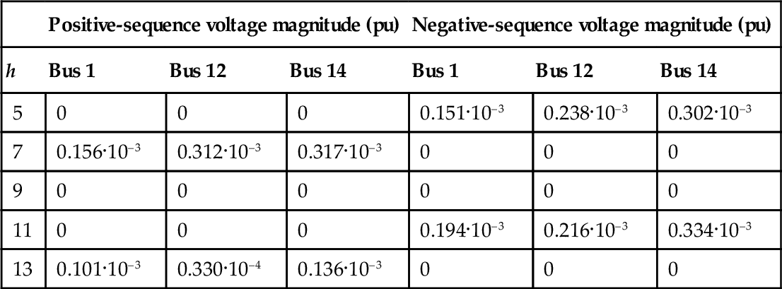
Table E4.11.3
Simulation Results for the 24-Bus System (Fig. E4.10.1): Negative-Sequence Fifth Harmonic Voltages at Different Buses
| Negative-sequence 5th harmonic voltage magnitude (pu) | ||
| Bus number | Simple model (Fig. 4.21) | New model (Fig. 4.25) |
| 1 | 0.161·10–3 | 0.151·10–3 |
| 2 | 0.161·10–3 | 0.151·10–3 |
| 3 | 0.161·10–3 | 0.151·10–3 |
| 4 | 0.184·10–3 | 0.184·10–3 |
| 5 | 0.184·10–3 | 0.184·10–3 |
| 6 | 0.185·10–3 | 0.179·10–3 |
| 7 | 0.185·10–3 | 0.179·10–3 |
| 8 | 0.141·10–3 | 0.147·10–3 |
| 9 | 0.259·10–3 | 0.257·10–3 |
| 10 | 0.269·10–3 | 0.268·10–3 |
| 11 | 0.281·10–3 | 0.279·10–3 |
| 12 | 0.229·10–3 | 0.238·10–3 |
| 13 | 0.268·10–3 | 0.268·10–3 |
| 14 | 0.302·10–3 | 0.302·10–3 |
| 15 | 0.247·10–3 | 0.246·10–3 |
| 16 | 0.292·10–3 | 0.296·10–3 |
| 17 | 0.279·10–3 | 0.279·10–3 |
| 18 | 0.265·10–3 | 0.269·10–3 |
| 19 | 0.276·10–3 | 0.276·10–3 |
| 20 | 0.224·10–3 | 0.224·10–3 |
| 21 | 0.200·10–3 | 0.208·10–3 |
| 22 | 0.237·10–3 | 0.246·10–3 |
| 23 | 0.233·10–3 | 0.241·10–3 |
| 24 | 0.194·10–3 | 0.201·10–3 |
| 25 | 0.119·10–3 | 0.119·10–3 |

4.3.4 Synchronous Machine Harmonic Model with Imbalance and Saturation Effects
This section introduces a synchronous machine harmonic model [12] that incorporates both frequency conversions and saturation effects under various machine load-flow constraints (e.g., unbalanced operation). The model resides in the frequency domain and can easily be incorporated into harmonic load-flow programs.
To model these effects and also to maintain an equivalent-circuit representation, a three-phase harmonic Norton equivalent circuit (Fig. 4.27) is developed with the following equations [12]:
[Ikm(h)]=[Y(h)]([Vh(h)]−[Vm(h)]−[E(h)])+[Inl(h)],
[E(h)]=0,ifh≠1[Ikm]=[Ikm−aIkm−bIkm−c]T[Vk]=[Vk−aVk−bVk−c]T[Vm]=[Vm−aVm−bVm−c]T[E]=[Epa2EpaEp]T[Inl]=[Inl−aInl−bInl−c]Ta=exp(−j2π/3)

where h is the harmonic order. In the model of Fig. 4.27, nonlinear effects are represented by a harmonic current source ([Inl(h)]) that includes the harmonic effects stemming from frequency conversion ([If(h)]) and those from saturation ([Is(h)]):
[Inl(h)]=[If(h)]+[IS(h)].

This harmonic model reduces to the conventional, balanced three-phase equivalent circuit of a synchronous machine if [Inl(h)] is zero and [Y(h)] is computed according to reference [65]. Since [Inl(h)] is a known current source (determined from the machine load-flow conditions), the model is linear and decoupled from a harmonic point of view. Therefore, it can be solved with network equations in a way similar to the traditional machine model.
To include the usual load-flow conditions, the following constraints are specified at the fundamental frequency (h = 1):
• Slack machine: The constraints are the magnitude and the phase angle of positive-sequence voltage at the machine terminals:
[T]([Vk]−[Vm])=Vspecified[T]=(1/3)[1aa2].

• PV machine: The constraints are the three-phase real power output and the magnitude of the positive-sequence voltage at machine terminals, where superscript H denotes conjugate transpose:
Real{−Ikm]H([Vk]−[Vm])}=Pspecified,
|[T]([Vk]–[Vm])|=Vspecified.
• PQ Machine: The constraints are the three-phase real and the three-phase reactive power outputs:
–[Ikm]H([Vk]–[Vm])=(P+jQ)specified.
These constraint equations and the machine structure equation (Eq. 4-51a) jointly define a three-phase machine model with nonlinear effects. Combining these equations with other network equations leads to multiphase load flow equations for the entire system [65]. The system is then solved by the Newton–Raphson method for each frequency. Detailed analysis and demonstration of Newton–Raphson based harmonic load flow is presented in Chapter 7.
In the model of Fig. 4.27, [Inl(h)] is not known and will be computed using the following iterative procedure:
• Step 1. Initialization
Set the harmonic current source [Inl(h)] to zero.
• Step 2. Network Load-Flow Solution
Replace the synchronous machines with their harmonic Norton equivalent circuits (Fig. 4.27) and solve the network equations for the fundamental and harmonic frequencies.
• Step 3. Harmonic Current-Source Computation Use the newly obtained network voltages and currents (from Step 2) to update [Inl(h)] for the machine equivalent circuit.
• Step 4. Convergence
If the computed [Inl(h)] values are sufficiently close to the previous ones stop; otherwise, go to Step 2.
The network load-flow solution and the harmonic iteration processes can be performed by any general purpose harmonic load-flow program as explained in Chapter 7 and reference [65]. Therefore, [Inl(h)] needs to be computed (Step 3). This will require the machine harmonic models in the dq0 and abc coordinates.
4.3.4.1 Synchronous Machine Harmonic Model Based on dq0 Coordinates
To incorporate the synchronous machine model (Fig. 4.27) in a general purpose harmonic analysis program, reasonable assumptions and simplifications according to the general guidelines indicated in references [66] and [67] are made. Under these assumptions, the following dq0 transformation is used to transfer the machine quantities from abc coordinates into rotating dq0 coordinates [12]:
[vdvqvo]T=[P]–1[vavbvc]T,
where
[P]−1=√2/3[cosθcos(θ−2π/3)cos(θ+2π/3)−sinθ−sin(θ−2π/3)−sin(θ+2π/3)√1/2√1/2√1/2].

In this equation θ = (ωt + δ) and δ is the angle between d-axis and the real axis of the network phasor reference frame. Defining
[D]=[1e−j2π/3e−j4π/3−j−je−j2π/3−je−j4π/3000]ejδ/√6[Do]=[000000√1/3√1/3√1/3],

matrix [P]–1 can be simplified as
[P]−1=[D]ejωt+[D]Ce−jωt+[Do].
Because the dq0 transformation is an orthogonal transformation, it follows that
[P]=([P]−1)T=[D]Teiωt+[D]He−jωt+[Do]T,
where superscripts T, C, and H represent transpose, conjugate, and conjugate transpose, respectively.
Using these equations for the dq0 transformation and the generator reference convention, a synchronous machine is represented in the dq0 coordinates as
[vpark]=−[R][ipark]−ddt[Ψpark]+[F][Ψpark][Ψpark]=[L][ipark],

where
[vpark]=[vdvqvovfvgvDvQ]T[ipark]=[idiqioifigiDiQ]T,[R]=[rarararfrgrDrQ]T[F]=[0−ω00000ω00000000000000000000000000000000000000000],[L]=[Ld00Mdf0MdD00Lq00Mgg0MgQ00Lo0000Mdf00Lff0MfD00Mqg00Lgg0MgQMdD00MfD0LDD00MqQ00MgQ0LQQ].

In these equations, subscripts f and D represent the field and damping windings of the d-axis, respectively, and subscripts g and Q indicate the field and damper windings of the q-axis, respectively.
Substituting Eq. 4-62 into Eq. 4-61 and defining the differential operator p=ddt:![]()
[vpark]=−[R][ipark]−p([L][ipark])+[F][L][ipark],=(−[R]−p[L]+[F][L])[ipark]=[Z(p)][ipark]

where [Z(p)] = –[R] – p(L) + [F][L] is the operation impedance matrix.
The rotor angular velocity (ω) is constant during steady-state operation; therefore, Eq. 4-63 represents a linear time-invariant system and can be written in the frequency domain for each harmonic hω, as follows:
[Vpark(h)]=[Z(h)][Ipark(h)].
For the harmonic quantities h ≠ 0 (e.g., excluding DC), the f, g, D, and Q windings are short-circuited; therefore, Eq. 4-64 can be rewritten as
[VdVqVo0000]=[⋮Z11(h)⋮Z12(h)⋮………⋮………⋮Z21(h)⋮Z22(h)⋮][IdIqIoIfIgIDIQ].

Solving for the dq0 currents as a function of the dq0 voltages, we have [12]:
[Idqo(h)]=[Z11(h)−Z12(h)Z22−1(h)Z21(h)]−1[Vdqo(h)]=[Ydqo(h)][Vdqo(h)],

where
[Ydqo(h)]=[Z11(h)−Z12(h)Z−122(h)Z21(h)]−1[Idqo(h)]=[IdIqIo]T[Vdqo(h)]=[VdVqVo]T
Equation 4-66 (consisting of a simple admittance matrix relating the dq0 components) defines the harmonic machine model in the dq0 coordinates.
For the DC components (e.g., h = 0), the voltage of the f-winding is no longer zero. Applying similar procedures, the results will be similar to Eq. 4-66, except that there is an equivalent DC voltage source (which is a function of the DC excitation voltage vf) in series with the [Ydq0] matrix.